HISTOPATHOLOGICAL IMAGE
CLASSIFICATION USING SALIENT POINT
PATTERNS
a thesis
submitted to the department of computer engineering
and the graduate school of engineering and science
of bilkent university
in partial fulfillment of the requirements
for the degree of
master of science
By
Celal C
¸ ı˘
gır
August, 2011
I certify that I have read this thesis and that in my opinion it is fully adequate, in scope and in quality, as a thesis for the degree of Master of Science.
Assist. Prof. Dr. C¸ i˘gdem G¨und¨uz Demir(Advisor)
I certify that I have read this thesis and that in my opinion it is fully adequate, in scope and in quality, as a thesis for the degree of Master of Science.
Assoc. Prof. Dr. ˙Ibrahim K¨orpeo˘glu
I certify that I have read this thesis and that in my opinion it is fully adequate, in scope and in quality, as a thesis for the degree of Master of Science.
Assist. Prof. Dr. ¨Ozlen Konu
Approved for the Graduate School of Engineering and Science:
Prof. Dr. Levent Onural Director of the Graduate School
ABSTRACT
HISTOPATHOLOGICAL IMAGE CLASSIFICATION
USING SALIENT POINT PATTERNS
Celal C¸ ı˘gır
M.S. in Computer Engineering
Supervisor: Assist. Prof. Dr. C¸ i˘gdem G¨und¨uz Demir August, 2011
Over the last decade, computer aided diagnosis (CAD) systems have gained great importance to help pathologists improve the interpretation of histopathological tissue images for cancer detection. These systems offer valuable opportunities to reduce and eliminate the inter- and intra-observer variations in diagnosis, which is very common in the current practice of histopathological examination. Many studies have been dedicated to develop such systems for cancer diagnosis and grading, especially based on textural and structural tissue image analysis. Al-though the recent textural and structural approaches yield promising results for different types of tissues, they are still unable to make use of the potential bio-logical information carried by different tissue components. However, these tissue components help better represent a tissue, and hence, they help better quantify the tissue changes caused by cancer.
This thesis introduces a new textural approach, called Salient Point Patterns (SPP), for the utilization of tissue components in order to represent colon biopsy images. This textural approach first defines a set of salient points that corre-spond to nuclear, stromal, and luminal components of a colon tissue. Then, it extracts some features around these salient points to quantify the images. Fi-nally, it classifies the tissue samples by using the extracted features. Working with 3236 colon biopsy samples that are taken from 258 different patients, our experiments demonstrate that Salient Point Patterns approach improves the clas-sification accuracy, compared to its counterparts, which do not make use of tissue components in defining their texture descriptors. These experiments also show that different set of features can be used within the SPP approach for better
iv
representation of a tissue image.
Keywords: Salient point patterns, texture, histopathological image analysis,
¨
OZET
¨
OZELL˙IKL˙I NOKTA MODELLER˙I KULLANARAK
H˙ISTOPATOLOJ˙IK RES˙IMLER˙IN
SINIFLANDIRILMASI
Celal C¸ ı˘gır
Bilgisayar M¨uhendisli˘gi, Y¨uksek Lisans Tez Y¨oneticisi: Y. Do¸c Dr. C¸ i˘gdem G¨und¨uz Demir
A˘gustos, 2011
Son on yıl i¸cinde, bilgisayar destekli te¸shis sistemleri, patologların kanser tespiti i¸cin histopatolojik g¨or¨unt¨uleri yorumlamasını artırmaya yardımcı olması y¨on¨uyle b¨uy¨uk bir ¨onem kazanmı¸stır. Bu sistemler, kanser tanısı i¸cin mevcut histopatolo-jik doku muayenesi uygulamasında ¸cok yaygın olan g¨ozlemci-i¸ci ve g¨ozlemciler arası de˘gi¸skenli˘gi azaltmaya ve ortadan kaldırmaya y¨onelik ¸cok de˘gerli fırsatlar sunmaktadır. ¨Ozellikle dokusal ve yapısal doku g¨or¨unt¨u analizine dayalı bir¸cok ¸calı¸sma, kanserin tanı ve sınıflandırması i¸cin bu t¨ur sistemleri geli¸stirmeye adanmı¸stır. Son zamanlardaki dokusal ve yapısal yakla¸sımlar, farklı tipte dokular i¸cin umut verici sonu¸clar vermesine ra˘gmen, doku bile¸senleri tarafından ta¸sınan potansiyel biyolojik bilgiyi kullanabilmekten yoksundurlar. Halbuki, bu doku bile¸senleri, doku temsiline ve dolayısıyla, kanserin yol a¸ctı˘gı doku de˘gi¸sikliklerini ¨
ol¸cmeye daha iyi yardımcı olur.
Bu tez, kolon biyopsi g¨or¨unt¨ulerini temsil etmede doku bile¸senlerinin kullanımı i¸cin ¨Ozellikli Nokta Modelleri olarak adlandırılan yeni bir dokusal yakla¸sım sun-maktadır. Bu dokusal yakla¸sım ¨oncelikle kolon dokusunun ¸cekirdek, stroma ve l¨umen bile¸senlerine kar¸sılık gelen bir dizi ¨ozellikli noktaları tanımlar. Sonra, bu belirgin noktalar etrafından doku g¨or¨unt¨ulerini ¨ol¸cmede kullanılan ¨oznitelikler ¸cıkartılır. Son olarak, bu ¨oznitelikleri kullanarak doku ¨orneklerini sınıflandırır. 258 farklı hastadan alınan 3236 kolon biyopsi ¨orne˘gi ¨uzerinde ger¸cekle¸stirdi˘gimiz deneyler, ¨Ozellikli Nokta Modelleri yakla¸sımının, dokuları tanımlamada yapısal bile¸senleri kullanmayan benzer ¸cal¸smalarla kar¸sıla¸stırıldı˘gında, sınıflandırma ba¸sarı y¨uzdesini artırdı˘gını ortaya koymu¸stur. Ayrıca ger¸cekle¸stirdi˘gimiz bu deneyler, doku g¨or¨unt¨us¨un¨un daha iyi temsil edilebilmesi i¸cin bu dokusal yakla¸sım
vi
kullanılarak farklı ¨ozniteliklerin elde edilebilece˘gini g¨ostermektedir.
Anahtar s¨ozc¨ukler : ¨Ozellikli nokta modelleri, yapısal doku, histopatolojik g¨or¨unt¨u analizi, otomatik kanser tanısı ve derecelendirilmesi, kolon kanseri.
Acknowledgement
This thesis would not have been possible without the guidance and the help of several people who contributed and extend their valuable assistance and support in the preparation and completion of this study.
First and foremost, I cannot find words to express my utmost gratitude to Assist. Prof. Dr. C¸ i˘gdem G¨und¨uz Demir whose sincerity, encouragement, and continuous support I will never forget. My special thanks goes to my thesis committee members, Assoc. Prof. Dr. ˙Ibrahim K¨orpeo˘glu and Assist. Prof. Dr. ¨Ozlen Konu, who have graciously agreed to serve on my committee. I would also like to thank Prof. Dr. Cenk S¨okmens¨uer for his consultancy on medical knowledge and Assist. Prof. Dr. Selim Aksoy for teaching Image Analysis course. Thanks to T ¨UB˙ITAK-B˙IDEB and T ¨UB˙ITAK-˙ILTAREN for their financial and research supports to me.
There are some people I would like to thank individually. I want to thank Ya¸sar Kemal Alp for being such a wonderful friend. It was a fabulous and ex-tremely quiet experience to be sharing a dormitory room with him for five years. I am extremely grateful to my friends for their help and encouragement: M¨ucahid Kutlu, Bahri T¨urel, Esat Belviranlı, Alptu˘g and Merve Dilek, Cem Aksoy, ¨Omer Faruk Uzar, Akif Burak Tosun, Erdem ¨Ozdemir, Hamza So˘gancı, Anıl Bayram, and Serdar Akbayrak. I would also like to acknowledge G¨ulden Olgun, Salim Arslan, and Can Koyuncu for allowing me to use their computers.
Last but not the least, I would like to thank my parents, Selver and Habip C¸ ı˘gır, and Aynur, my future wife, for their endless support and love. I will be forever grateful to them.
This thesis is dedicated to people who devoted themselves to my country.
Celal C¸ ı˘gır August, 2011
Contents
1 Introduction 1
1.1 Motivation . . . 4
1.2 Contribution . . . 7
1.3 Organization of the Thesis . . . 8
2 Background 9 2.1 Medical Background . . . 9
2.2 Automated Histopathological Image Analysis . . . 11
2.2.1 Tissue image segmentation . . . 11
2.2.2 Medical image retrieval . . . 12
2.2.3 Histopathological image classification . . . 14
2.3 SIFT Key Points . . . 16
3 Methodology 21 3.1 Salient Point Identification . . . 22
CONTENTS ix
3.1.1 Clustering . . . 23
3.1.2 Type assignment . . . 24
3.1.3 Salient points . . . 26
3.2 Salient Point Patterns . . . 27
3.3 Feature Extraction . . . 31
3.3.1 Color histogram features . . . 31
3.3.2 Co-occurrence matrix features . . . 32
3.3.3 Run-length matrix features . . . 34
3.3.4 Local binary pattern features . . . 35
3.3.5 Gabor filter features . . . 36
3.4 Tissue Classification . . . 37
3.4.1 Support vector machines (SVM) . . . 38
3.4.2 Cross-validation . . . 39
4 Experimental Results 41 4.1 Experimental Setup . . . 41
4.2 Comparison Criteria . . . 42
4.3 Results and Comparisons . . . 43
4.3.1 Parameter selection . . . 43
4.3.2 Color histogram features . . . 44
CONTENTS x
4.3.4 Run-length matrix features . . . 50
4.3.5 LBP histogram features . . . 52
4.3.6 Gabor filter features . . . 55
4.3.7 Parameter analysis . . . 57
4.4 Discussion . . . 64
4.4.1 Parameters . . . 64
4.4.2 Features . . . 64
List of Figures
1.1 Distribution of deaths by leading cause groups, males and females, worldwide, 2004. . . 2
1.2 Ten leading cancer types for estimated new cancer cases and deaths, by sex, United States, 2011 . . . 3
1.3 Histopathological images of colon tissues, which are stained with the routinely used hematoxylin-and-eosin technique. . . 6
2.1 Cellular, stromal, and luminal components of a colon tissue stained with the hematoxylin-and-eosin technique. . . 10
2.2 The initial image is repeatedly convolved with Gaussians to pro-duce the set of scale space images shown on the left. Adja-cent Gaussian images are subtracted to produce the difference-of-Gaussian images on the right. After each octave (an octave corresponds to doubling the value of σ), the Gaussian image is down-sampled by a factor of 2, and the process repeated. . . 17
2.3 DOG images in different scales and octaves: (a) Normal, (b) low-grade cancerous, and (c) high-low-grade cancerous colon tissues. Their corresponding DOG images in different scales and octaves are (d), (e), and (f), respectively. The SIFT keypoints defined on (a) are presented in (g). . . 19
LIST OF FIGURES xii
3.1 The flowchart of the proposed histopathological image processing system. . . 22
3.2 Examples of colon tissue images and resulting k-means clusters. . 25
3.3 Examples of colon tissues and resulting circle-fit representation. . 28
3.4 Some Salient Point Patterns (SPP) on a normal colon tissue. Here yellow, cyan, and blue circles correspond to examples of lumen, stroma, and nuclei components, respectively. . . 29
3.5 The accumulated co-occurrence matrix computed over those when
d is selected as 1. . . . 33
3.6 Run-length matrices derived from a gray level image (G = 3) in dif-ferent orientations. Rows represent the gray level of a run, columns represents the length of the run. The accumulated run-length ma-trix is also shown. . . 34
3.7 Illustration of extraction an LBP features. . . 35
3.8 Rotation invariant binary patterns with white and black circles correspond to 0 and 1 in the output of the LBP operator. The numbers inside them correspond to the respective bin numbers. . 36
3.9 Two different hyperplane constructed by a support vector classifier. 38
4.1 Classification accuracies as a function of the number of bins N when the SPP method uses the color histogram features. Here the circular window radius R is fixed to 10. . . . 58
4.2 Classification accuracies as a function of the circular window radius
R when the SPP method uses the color histogram features. Here
LIST OF FIGURES xiii
4.3 Classification accuracies as a function of the number of bins N when the SPP method uses the co-occurrence matrix features. Here the distance parameter d and the circular window radius pa-rameter R are fixed to 10 and 30, respectively. . . . 59
4.4 Classification accuracies as a function of the distance d when the SPP method uses the co-occurrence matrix features. Here the number of bins parameter N and the circular window radius pa-rameter R are fixed to 8 and 30, respectively. . . . 60
4.5 Classification accuracies as a function of the circular window radius
R when the SPP method uses the co-occurrence matrix features.
Here the number of bins parameter N and the distance parameter
d are fixed to 8 and 10, respectively. . . . 61
4.6 Classification accuracies as a function of the number of bins N when the SPP method uses the run-length matrix features. Here the circular window radius R is fixed 20. . . . 62
4.7 Classification accuracies as a function of the circular window radius
R when the SPP method uses the run-length matrix features. Here
the number of bins N is fixed 64. . . . 62
4.8 Classification accuracies as a function of the circular window radius
R when the SPP method uses the LBP histogram features. . . . . 63
4.9 Classification accuracies as a function of the circular window radius
List of Tables
3.1 The intensity-based features defined on the gray level histogram. . 32
3.2 The textural features derived from a co-occurrence matrix. . . 33
3.3 The textural features derived from run-length matrices. In this table, p is the number of pixels in an image and n =∑i∑jR(i, j). 35
4.1 Number of colon tissue images in the training and test sets. . . . 42
4.2 The list of the parameters issued during feature extraction and classification steps. . . 44
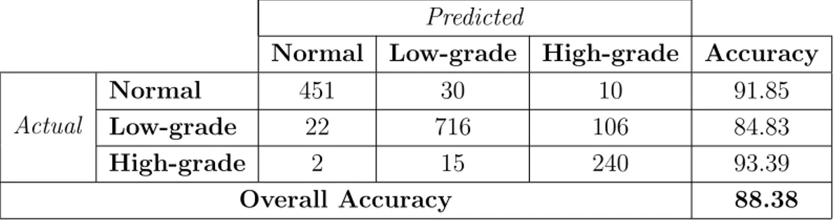
4.3 The confusion matrix and the accuracies obtained by the color histogram features when the EntireImageApproach is used. . . . . 45
4.4 The confusion matrix and the accuracies obtained by the color histogram features when the GridPartitionApproach is used. . . . 45
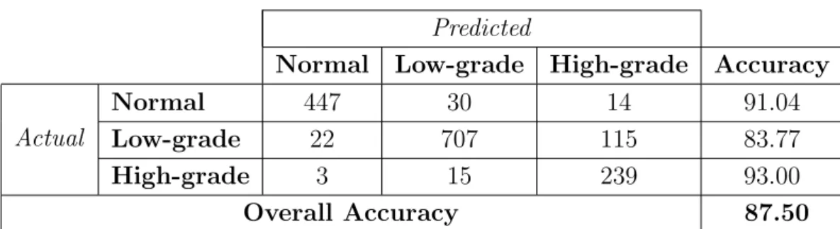
4.5 The confusion matrix and the accuracies obtained by the color histogram features when the SIFTPointsApproach is used. . . . . 46
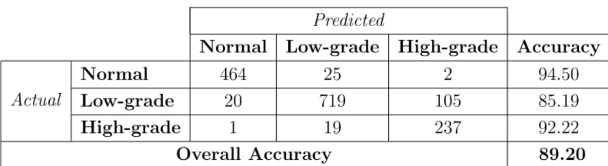
4.6 The confusion matrix and the accuracies obtained by the color histogram when the proposed SPP method is used. . . 46
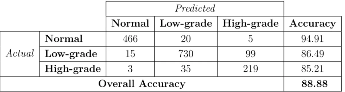
4.7 The confusion matrix and the accuracies obtained by the color histogram features when the TypelessApproach is used. . . . 47
LIST OF TABLES xv
4.8 The confusion matrix and the accuracies obtained by the co-occurrence matrix features when the EntireImageApproach is used. 48
4.9 The confusion matrix and the accuracies obtained by the co-occurrence matrix features when the GridPartitionApproach is used. 48
4.10 The confusion matrix and the accuracies obtained by the co-occurrence matrix features when the SIFTPointsApproach is used. 48
4.11 The confusion matrix and the accuracies obtained by the co-occurrence matrix features when the proposed SPP method is used. 49
4.12 The confusion matrix and the accuracies obtained by the co-occurrence matrix features when the TypelessApproach is used. . . 50
4.13 The confusion matrix and the accuracies obtained by the run-length matrix features when the EntireImageApproach is used. . . 51
4.14 The confusion matrix and the accuracies obtained by the run-length matrix features when the GridPartitionApproach is used. . 51
4.15 The confusion matrix and the accuracies obtained by the run-length matrix features when the SIFTPointsApproach is used. . . 51
4.16 The confusion matrix and the accuracies obtained by the run-length matrix features when the proposed SPP method is used. . 52
4.17 The confusion matrix and the accuracies obtained by the run-length matrix features when the TypelessApproach is used. . . . . 52
4.18 The confusion matrix and the accuracies obtained by the LBP histogram features when the EntireImageApproach is used. . . . . 53
4.19 The confusion matrix and the accuracies obtained by the LBP histogram features when the GridPartitionApproach is used. . . . 53
LIST OF TABLES xvi
4.20 The confusion matrix and the accuracies obtained by the LBP histogram features when the SIFTPointsApproach is used. . . . . 54
4.21 The confusion matrix and the accuracies obtained by the LBP histogram features when the proposed SPP method is used. . . 54
4.22 The confusion matrix and the accuracies obtained by the LBP histogram features when the TypelessApproach is used. . . . 54
4.23 The confusion matrix and the accuracies obtained by the Gabor filter features when the EntireImageApproach is used. . . . 55
4.24 The confusion matrix and the accuracies obtained by the Gabor filter features when the GridPartitionApproach is used. . . . 56
4.25 The confusion matrix and the accuracies obtained by the Gabor filter features when the SIFTPointsApproach is used. . . . 56
4.26 The confusion matrix and the accuracies obtained by the Gabor filter features when the proposed SPP method is used. . . 56
4.27 The confusion matrix and the accuracies obtained by the Gabor filter features when the TypelessApproach is used. . . . 57
4.28 Classification results obtained for the color histogram features. . . 65
4.29 Classification results obtained for the co-occurrence matrix features. 65
4.30 Classification results obtained for the run-length matrix features. . 66
4.31 Classification results obtained for the LBP histogram features. . . 66
4.32 Classification results obtained for the Gabor filter features. . . 66
5.1 Classification results obtained by the proposed Salient Point Pat-terns (SPP) method for different features. . . 68
Chapter 1
Introduction
Cancer, also named as malignant neoplasm, is the name for a group of diseases characterized by the uncontrolled growth and spread of abnormal cells. Around the world, cancer is ranked the third leading cause of deaths following cardio-vascular and infectious diseases. In respect of percentage, such diseases caused almost 13.4 percent of all deaths in men and 11.8 percent in women in 2004 [6]. As it is presented in Figure 1.1, cancer causes more deaths than respiratory dis-eases, diabetic disdis-eases, and deaths because of perinatal conditions; furthermore cancer results in more deaths than HIV/AIDS, tuberculosis, and malaria which lie in infectious diseases.
Normally, body cells grow over time and new cells take place when old ones die. However, cancer cells grow and divide without dying and form new abnormal cancer cells. At the end, these cells group together and form an additional mass of tissue. This mass is called a malignant tumor. Prostate, breast, lung, and colorectal cancers are some of the cancer types that form a malignant tumor. Some cancers, like leukemia, do not form tumors. Instead, these cancer cells divide irregularly causing increase in white blood cells [1].
Being a tumor-forming cancer type, colon cancer is one of the most common types of cancer that afflicts many people each year. It is also called as colorectal cancer or large bowel cancer. According to American Cancer Society research in
CHAPTER 1. INTRODUCTION 2
Figure 1.1: Distribution of deaths by leading cause groups, males and females, worldwide, 2004.1
2011, about 1.5 million new cancer cases will occur in the U.S. and colon cancer is estimated as the third most common cancer type for both males and females [63]. As it is shown in Figure 1.2, 9 percent of new cancer cases will be type of colorectal cancer and unfortunately, 34 percent of them will result in death for both males and females.
Colon cancer grows in the wall of the colon. Most begin as a small growth on the bowel wall. These growths are usually benign (not cancerous), but some develop into cancer over time. The process of forming tumor in the colon wall can take many years, which allows time for early detection with screening tests. Widespread screening tests play an important role to identify cancers at an early and potentially treatable stage [64]. In order to select the correct treatment plan, cancer must be diagnosed and graded accurately. For cancer diagnosis, there are many methods that are employed in clinical institutions. Blood and urine tests are one of these methods to make cancer diagnosis and they give
CHAPTER 1. INTRODUCTION 3
Figure 1.2: Ten leading cancer types for estimated new cancer cases and deaths, by sex, United States, 2011.2
the pathologists beneficial information about the effects of the disease on the body. Medical imaging techniques, such as X-ray images, magnetic resonance imaging (MRI), and ultrasonography are used to detect different types of cancer [4, 11, 26, 31, 64, 65]. Genetic testing is another technique for cancer diagnosis but due to complexity of testing, cost, and a requirement for specialists make it hard to apply for practical use in clinical institutions [17, 52].
Although all these screening methods are used to detect cancer, the final diagnosis are made with histopathological tissue examination. Moreover, these aforementioned screening methods are not capable of making reliable grading,
2Source: Siegel R. et al. Cancer statistics, 2011. CA: A Cancer Journal for Clinicians, 61(4):212236, 2011.
CHAPTER 1. INTRODUCTION 4
and hence, histopathological tissue examination should be done [9, 12, 58]. In clinical medicine, histopathology refers to the examination of a biopsy (a sample tissue) or a surgical specimen by a pathologist, after histological sections have been stained with a special technique to enhance contrast in the microscopic image and placed onto glass slides. In this examination, pathologists visually examine the changes in cell morphology and tissue distribution under a microscope. If a cancerous region is found in a tissue sample, a grade is assigned to the tissue to characterize the degree of its malignancy.
Conventional histopathological examination in cancer diagnosis is prone to subjectivity and may lead to a considerable amount of intra- and inter-observer variation and poor reproducibility, due to its heavy reliance on human interpre-tation [3, 33, 46]. Moreover, it is a time-consuming process to examine the whole specimen for making a decision. Computer-aided diagnosis (CAD), therefore, has been proposed to eliminate variations among pathologists and decrease the sub-jectivity level by assisting pathologists with making more reliable decisions in a time-saving way.
1.1
Motivation
In literature, there have been many studies to develop CAD systems to assist pathologists in their evaluations of histopathological images. In these studies, a tissue is represented with a set of mathematical features that is used in automated diagnosis and grading process. In order to extract these features, there are mainly four different approaches. These are intensity-based, textural, tissue component-based (morphological), and structural approaches.
In the intensity-based approach, a tissue is quantified with the statistical distributions of gray level or color intensities of its pixels. This approach first computes a color or gray level histogram of a tissue image by quantizing its pixels into bins and then, defines a set of statistical features on the histogram [11, 65, 67]. However, intensity distributions are similar for different types of
CHAPTER 1. INTRODUCTION 5
tissues stained with the hematoxylin-and-eosin staining technique. Moreover, this approach is not capable of capturing spatial relations of tissue components as visual descriptors of the images.
In the textural approach, tissue images are represented with a set of features that can be calculated from co-occurrence matrices [16, 29, 19, 60], run-length matrices [44, 74], multiwavelet coefficients [32, 74], fractal geometry [20, 72], and local binary patterns (LBP) [41, 61, 65]. Since texture definition is made on pixels, it is sensitive to noise in the pixel values.
In the morphological approach, a tissue is represented with the size, shape, orientation, and other geometric properties of the tissue components. These properties are measured defining morphological features such as area, perime-ter, roundness, and symmetry [72, 67]. This approach requires identifying exact boundaries of cells before extracting the features. Due to complex nature of histopathological images, it is hard to locate tissue components and this leads to a difficult segmentation problem.
Structural approach characterizes the tissue with the spatial distribution of its cellular components. A tissue is represented as a graph and a set of structural features is extracted from this graph representation. The locations of the cell nuclei are considered as nodes to generate such graphs including Delaunay trian-gulations and their corresponding Voronoi diagrams [18, 74], minimum spanning trees [75], and probabilistic graphs [15, 27].
Although the recent textural and structural approaches for the development of CAD systems yield promising results for different types of tissues, they are still unable to make use of the potential biological information carried by the tissue components. However, these tissue components help better represent a tissue, and hence, they help better quantify the tissue changes due to existence of cancer. For example, in typical colon tissues, epithelial cells are arranged in an order around a luminal structure to form a glandular structure and non-epithelial cells take place in stroma found in between these glands. The gland structures for normal colon tissues are presented in Figures 1.3(a) and 1.3(b). This gland formation deviates from its regular structure due to existence of cancer. At
CHAPTER 1. INTRODUCTION 6
(a) (b)
(c) (d)
(e) (f)
Figure 1.3: Histopathological images of colon tissues, which are stained with the routinely used hematoxylin-and-eosin technique: (a)-(b) normal, (c)-(d) low-grade cancerous, and (e)-(f) high-low-grade cancerous.
CHAPTER 1. INTRODUCTION 7
the beginning, the degree of distortion is lower such that gland formations are well to moderately differentiated; examples of low-grade cancerous tissues are shown in Figures 1.3(c) and 1.3(d). Then, the distortion level becomes higher such that the gland formations are poorly differentiated. Figures 1.3(e) and 1.3(f) present such high-grade cancerous colon tissue samples. The quantification of these deviations in glandular structure is very important for accurate cancer grading. In addition to its nuclear components, luminal and stromal regions make easier the quantification of the distortions.
1.2
Contribution
Pathologists visually examine the spatial relations of tissue components such as stroma, nuclei, and lumen for cancer diagnosis and grading. However, most of the textural and structural approaches use only the information provided by nuclear region, ignoring the potential information provided by luminal or stromal regions. On the other hand, it is beneficial to use these tissue components all together for better characterization of a tissue.
In this thesis, we introduce a new textural method, called Salient Point Pat-terns (SPP), for the utilization of tissue components in order to represent colon biopsy images. For this purpose, first a set of salient points is defined to approx-imately represent the tissue components including nuclei, stroma, and lumen. Then, a circular window centered on the centroids of the components is used as a mask to extract different types of features around these salient points. Finally, tissue classification is performed by using the extracted set of features. Our ex-periments demonstrate that this classification approach leads promising results for differentiating normal, low-grade cancerous, and high-grade cancerous tissue images. The main contribution of this thesis can be summarized as the use of salient points to represent tissue components in texture definition. Moreover, the SPP method has a potential of being applied for other types of cancer such as prostate and skin cancer.
CHAPTER 1. INTRODUCTION 8
1.3
Organization of the Thesis
This thesis is organized as follows: In Chapter 2, we give an overview of the medical background information about cancer and the earlier research related to classification of histopathological images. In Chapter 3, we explain the proposed Salient Point Patterns method in detail. Consequently, in Chapter 4, we describe the experiments and analyze the experimental results. Finally, we summarize our work and discuss its future research aspects in Chapter 5.
Chapter 2
Background
This chapter presents the background information about histopathological image analysis. First of all, general information about colon tissues, the staining process, and changes in colon tissues caused by colon cancer are mentioned. Following the medical background, a brief summary of the previous studies about histopatho-logical image classification for cancer grading and diagnosis is presented. Finally, SIFT key point descriptor, a method for detecting interest points in tissue images, is mentioned.
2.1
Medical Background
The colon, sometimes referred to as the large intestine or large bowel, is a long, hollow tube at the end of the digestive tract. Its main role can be defined as a waste processor; taking digested food in the form of solid waste and pushing it out of the body through the rectum and anus. It absorbs water, electrolytes and nutrients from food and transports them into the bloodstream.
If a doctor suspects cancer in colon, he or she needs to know the status of the colon tissues. In a current clinical practice, histopathological examination is the
CHAPTER 2. BACKGROUND 10
routinely applied method for diagnosis and grading of colon cancer. Histopatho-logical examination of tissues starts with removing a sample of a small amount of tissue. This procedure is called biopsy. The sample tissue or surgical specimen is to be examined under a microscope by a pathologist. Before the microscopic examination, histological sections have been taken from the biopsy and stained with special chemicals in order to enhance contrast in the microscopic image.
Hematoxylin-and-eosin (H&E) is the routinely used technique for staining tis-sues at clinical institutions. In a typical tissue, hematoxylin colors nuclei of cells with blue-purple hue, whereas alcoholic solution of eosin colors eosinophilic struc-tures such as proteins and cytoplasms with pink [22]. Therefore, a biopsy tissue stained with the hematoxylin-and-eosin technique has large amounts of different levels of blue-purple, pink, and white components. In Figure 2.1, a sample colon tissue stained with the hematoxylin-and-eosin technique is presented. In a typ-ical colon tissue, there are epithelial cells and stromal cells. An epithelial cell consists of a nucleus, dark purple region, and a cytoplasm, white region near the epithelial cell nucleus. A sample epithelium cell is marked with a red solid circle in the figure. A group of epithelium cells is lined up around a luminal region to form a glandular structure; a luminal area and a gland border are also marked in this figure. Stromal cells are not part of the glandular structures. They are connective tissue components that hold all of the structures in the tissue together.
Figure 2.1: Cellular, stromal, and luminal components of a colon tissue stained with the hematoxylin-and-eosin technique.
CHAPTER 2. BACKGROUND 11
Colon adenocarcinoma, which accounts for 90-95 percent of all colorectal cancers, originates from the lining of the large intestine causing organizational changes in the glandular structure of the colon tissue. In order to determine the most appropriate treatment plan, cancer should be diagnosed and graded accurately. For colon adenocarcinoma, grading is a description of how closely a colorectal gland looks like a normal gland. It scales the distortions in the or-ganization of the colon tissue. In low-grade cancerous tissues, gland formations are well to moderately differentiated. However, in high-grade cancerous tissues, gland formations are only poorly differentiated [21]. In this thesis, we consider classifying a tissue image as normal, low-grade cancerous, or high-grade cancer-ous.
2.2
Automated Histopathological Image
Analysis
In literature, there have been several studies related to the development of CAD systems for histopathological image analysis. These studies can be broadly di-vided into three main groups based on their purpose: tissue image segmentation, retrieval, and classification.
2.2.1
Tissue image segmentation
Segmentation is the initial step in histopathological image analysis. Here, the aim is to divide a heterogenous image into its homogeneous parts. These ho-mogeneous parts can later be used by classification algorithms. To identify the homogenous regions in an image, many approaches have been proposed. Tosun
et al. [70] proposed a new algorithm for an unsupervised segmentation of colon
biopsy images. In their algorithm, they first run k-means clustering on the color intensities of pixels to cluster them into three main groups: purple for epithelial and lymphoid cell nuclei regions, pink for connective tissue regions and epithelial
CHAPTER 2. BACKGROUND 12
cell cytoplasm and white for luminal structures, connective tissue regions, and epithelial cell cytoplasm. Then, they define circular primitives on the pixels of each cluster and define a descriptor on these primitives that is to be used in a re-gion growing algorithm. In their recent study, they introduced another descriptor that is used for histopathological image segmentation [69]. In this study, graphs are used to quantify the relations of tissue components.
Kong et al. applied clustering-based segmentation on whole slide histology images [36]. They first divide a whole slide image of neuroblastoma tumor into tiles and each image tile is segmented into five salient components: nuclei, cy-toplasm, neuropil, red blood cells, and background. Segmentation is performed by constructing a feature vector that combines color and entropy information extracted from the RGB and La*b* color spaces and classifying this vector into one of the components.
Image filtering is also proposed for segmentation of colon biopsy images [78]. In this study, a directional 2D filter is applied to an image. Each directional 2D filter detects the chain segment in a particular direction and gland segmentation is performed on these filter responses. Image thresholding on the color intensities of pixels followed by iterative region growing is another approach for segmentation of histopathological images [77]. Naik et al. proposed to use a Bayesian classifier on pixel values to detect nuclei, cytoplasm, and lumen components in prostate tissue images [47, 48]. They manually select a set of pixel values representing each of the three classes as the ground truth. Then, pixels in a tissue image are labeled using a Bayesian classifier after applying an empirically determined threshold. Finally, a region that corresponds to a set of connected pixels in the same cluster is considered as a segmented region.
2.2.2
Medical image retrieval
With the development of medical imaging and computer technology, there is an exponential increase in the amount of medical images and this makes the management, maintenance, and retrieval of medical images more difficult. This
CHAPTER 2. BACKGROUND 13
fact leads researchers to work on medical image retrieval systems [43]. Such systems are designed for accessing the most visually similar images to a given query image from a database of images.
ASSERT [62] is one of the medical image retrieval systems that mainly focus on the computed tomography (CT) images of lung. Image Retrieval in Medical Applications (IRMA) [34] system is designed for the classification of images into anatomical areas. Traditional content-based medical image retrieval is based on low level features such as color, texture, shape, spatial relationships, and mixture of these [43, 79, 83, 85]. On the other hand, recent studies have focused on the semantic content analysis of medical images in order to improve the retrieval performance [8, 68, 80]. Tang et al. propose I-Browse system that is specialized for retrieval of gastrointestinal tract images [68]. They manually assign semantic labels to the subimages with the help of histopathologists to form ground truth image patches. Then, a set of Gabor features and gray level mean and deviations of the normalized histogram of these subimages are extracted to construct features in image retrieval process. Caicedo et al. propose a semantic content-based image retrieval for histopathology images [8]. They first extract low level features, such as gray/color histogram, edge histogram, and texture histogram features, on images of special skin cancer called basal-cell carcinoma. Then, these low level features are mapped to high-level features that reflect the semantic content of the images with help of pathologists.
The evaluation of content-based medical image retrieval performance is usu-ally done by measuring precision and recall values defined as follows [43]:
precision = number of relevant items retrieved
number of items retrieved (2.1)
recall = number of relevant items retrieved
CHAPTER 2. BACKGROUND 14
2.2.3
Histopathological image classification
Many studies have been proposed to classify histopathological images in order to support pathologists in their evaluations. In these studies, tissue images are rep-resented with a set of mathematical features. In literature, there are mainly four different approaches to extract mathematical features for tissue representation. These are morphological, intensity-based, textural, and structural approaches.
In the morphological approaches, a tissue is represented with the size, shape, orientation, and other geometric properties of its cellular components. How-ever, this approach requires segmentation of tissue components before hand. One of the earliest studies based on morphological features is done by Street et al. [66]. They first segment the nucleus components of breast tumor tissues in a semi-automated way. Then, they define morphological features such as radius, perimeter, area, compactness, smoothness, concavity, and symmetry. Masood
et al. use morphological features to represent cellular components of the colon
tissues [42]. Such components are nuclei, cytoplasm, glandular structures, and stromal regions, which are segmented by applying k-means clustering on color intensities of a colon tissue image. Rajpoot et al. extract morphological features such as area, eccentricity, average diameter, Euler number, orientation, solidity, major axis length, and minor axis length for colon tissue cell representations [55]. Moreover, morphological features are commonly used in cancer diagnosis [11, 18, 45, 47, 67, 72]. Here are the definitions of some of these morphological features :
• Area: The number of pixels in the region.
• Perimeter: The total length of the region boundaries.
• Radius: The radius of a circle with the same area as the region.
• Compactness: The measure of the compactness of the region using the
formula perimeter2/area.
CHAPTER 2. BACKGROUND 15
• Minor axis length: The length of the axis that is orthogonal to the major
axis of the region.
In the intensity-based approach, gray level or color intensities of pixels are used to quantify a tissue image. First, color histogram is computed by putting the pixels of the image into bins and then, features such as mean, standard deviation, skewness, kurtosis, and entropy are defined on this histogram [11, 76, 18]. However, this type of features does not include any information about the spatial distributions of tissue components or pixels.
In the textural approach, the texture of an entire tissue or tissue components is quantified by computing different textural features derived from co-occurrence matrices, run-length matrices, Gabor filters, and fractal dimension analysis. Co-occurrence matrices are widely used tools to extract textural descriptors for histopathological image analysis [16, 18, 19, 29, 60, 72]. Doyle et al. use co-occurrence matrices and Gabor filter responses to represent prostate tissue images for cancer grading [18]. Waheed et al. performe textural analysis on renal cell carcinoma by computing fractal dimension features together with co-occurrence features on an entire image as well as on an individual cellular structures [72]. Esgiar et al. study on the textural analysis of cancerous colonic mucosa [19]. They first compute a co-occurrence matrix on gray-level tissue images. Then, angular second moment to characterize the homogeneity of the image, difference moment to measure local variation, correlation function to calculate the linearity of the gray-level dependencies, entropy to measure randomness, inverse difference moment to identify the local homogeneity of the image and dissimilarity to mea-sure the degree of dissimilarity between pixels are computed on the co-occurrence matrix.
In the structural approach, a tissue is represented with the spatial distribu-tions of its cellular components. Graph representation is made on the tissue components and a set of structural features is derived on this graph. Doyle et
al. employed Delanuay triangulations, minimum spanning trees, and Voronoi
diagrams to describe spatial arrangement of the nuclei on prostate tissue im-ages [18]. Features are derived from these graphs including area, the disorder of
CHAPTER 2. BACKGROUND 16
the area, and roundness factor on a Voronoi diagrams together with the average edge length and maximum edge length on Delanuay triangulations. Altunbay et
al. propose color graphs for representing colon tissue images [2]. They initially
segment nuclear, stromal, and luminal regions from a tissue image and identify their centroids as graph nodes. Then, a Delanuay triangulation is constructed on these nodes by assigning different colors to the edges depending on the compo-nent types of their end nodes. Finally, the colored-version of the average degree, average clustering coefficient, and diameter are extracted to quantify the graph, and thus, to represent the tissue.
Moreover, recent studies on histopathological images focus on the local salient points that contain more information about the underlying medical structure. Raza et al. propose a CAD system for classification of renal cell carcinoma sub-type using the scale invariant feature transform (SIFT) features [57]. In their next study [56], they use the SIFT features to decompose an image into a col-lection of small patches and then, apply k-means to cluster these small patches. Finally, they represent an image as the number of descriptors assigned to each cluster, called bag-of-features. Caicedo et al. employ the SIFT keypoints for con-struction of the codebook to represent histopathological image contents [7]. D´ıaz
et al. apply the SIFT algorithm to represent local patches that correspond to
nuclear structures in skin biopsy images [14].
2.3
SIFT Key Points
Lowe propose a SIFT (Scale Invariant Feature Transform) method for extracting distinctive features that characterize a set of keypoints for an image [39]. The keypoints are shown to be scale and orientation invariant. Therefore, SIFT is used in many studies such as object recognition, image matching applications, and image retrieval applications.
There are four major stages of computation that the SIFT algorithm uses to generate the set of image features :
CHAPTER 2. BACKGROUND 17
Figure 2.2: The initial image is repeatedly convolved with Gaussians to produce the set of scale space images shown on the left. Adjacent Gaussian images are subtracted to produce the difference-of-Gaussian images on the right. After each octave (an octave corresponds to doubling the value of σ), the Gaussian image is down-sampled by a factor of 2, and the process repeated.
1. Scale-space extreme detection: Potential interest points are identified by scanning an image over locations and scales. The keypoints are the local peaks or extreme points in the scale space of the image generated by applying Difference-of-Gaussian (DoG) functions to the image. The scale space of the image is defined as a function, L(x, y, σ), that is produced by convolving the input image, I(x, y), with variable scale Gaussian function
G(x, y, σ):
L(x, y, σ) = G(x, y, σ)∗ I(x, y) (2.3)
where ∗ is the convolution operation and G(x, y, σ) is a Gaussian function defined as:
G(x, y, σ) = 1
2πσ2e
−(x2+y2)/2πσ2
(2.4)
A DOG scale space function D(x, y, σ) can be computed from the difference of two scales separated by a constant multiplicative factor of k:
D(x, y, σ) = (G(x, y, kσ)− G(x, y, σ)) ∗ I(x, y) (2.5) = L(x, y, kσ)− L(x, y, σ)
CHAPTER 2. BACKGROUND 18
An efficient approach to construct DOG images is shown in Figure 2.2. First, an initial image I is convolved with a Gaussian function, G0, of
width σ0. Resulting image, L, is the blurred version of the original image.
Then, this blurred image is incrementally convolved with a Gaussian, Gi,
of width σi to generate the ith image in the stack, which is equivalent to
the original image convolved with a Gaussian Gk, of width kσ0. Adjacent
image scales are subtracted to produce the Difference-of-Gaussian images as shown on the right side of the figure.
2. Accurate keypoints localization: This stage is to determine a detailed model of location and scale for each candidate location. Least square fitting is conducted via Taylor expansion of the scale-space function, D(x, y, σ), so that the origin is at the sample point:
D(X) = D + ∂D T ∂X X + 1 2X T∂2D ∂X2X (2.6)
where X = (x, y, σ)T is the offset from this point. Then, keypoints at the
location are located and scaled by calculating the extreme of the fitted surface. The keypoints are eliminated if they are found unstable during the computation.
3. Orientation assignment: Each keypoint location is assigned to several
orientations that is based on local image gradient directions in a scale in-variant manner. For each image sample, L(x, y), at scale of the keypoint, the gradient magnitude, m(x, y), and orientation, θ(x, y), is computed using pixel differences:
m(x, y) = √
(L(x + 1, y)− L(x − 1, y))2+ (L(x, y + 1)− L(x, y − 1))2
θ(x, y) = tan−1((L(x, y + 1)− L(x, y − 1))/(L(x + 1, y) − L(x − 1, y)) An orientation histogram, which has 36 bins covering the 360 degree, is formed from the gradient orientations. Finally, orientation of the highest magnitude is assigned to the keypoint.
4. Keypoints descriptor: A descriptor for each keypoint is created. First of all, the coordinates of the descriptor and gradient orientations are rotated
CHAPTER 2. BACKGROUND 19
Figure 2.3: DOG images in different scales and octaves: (a) Normal, (b) low-grade cancerous, and (c) high-low-grade cancerous colon tissues. Their corresponding DOG images in different scales and octaves are (d), (e), and (f), respectively. The SIFT keypoints defined on (a) are presented in (g).
CHAPTER 2. BACKGROUND 20
relative to the keypoint orientation in order to achieve rotation invariance. Using the scale of the keypoint, the pixels in the 16× 16 neighborhood of the keypoint location are divided into 4× 4 windows. The gradient vectors are accumulated into 8 orientation bins resulting in 128 descriptors for each keypoint. Then, the vector is normalized to make it invariant to illumination changes.
An example of DOG images generated from the colon biopsy tissue images can be found in Figure 2.3.
Chapter 3
Methodology
In previous chapters, we mentioned that histopathological examination is prone to subjectivity and may lead to a considerable amount of intra- and inter-observer variation due to its heavy reliance on pathologist interpretation. To eliminate the subjectivity level, and therefore, to help pathologists make more accurate decisions, computer-aided diagnosis (CAD) has been proposed. There have been many studies and methods on the construction of CAD systems as presented in Chapter 2. However, these studies usually discard the domain specific knowl-edge and treat histopathological images as generic images. In this chapter, we introduce a new method, called Salient Point Patterns (SPP), to characterize the histopathological images with its tissue components: nuclei, stroma and lumen.
The proposed method is composed of a series of processing steps. The first step begins with clustering the pixels of an image into three groups, which correspond to nuclear (purple), stromal (pink), and luminal (white) areas using the k -means clustering algorithm. Then, postprocessing is applied on the pixels of each cluster to decrease the effects of noise due to incorrect clustering of pixels. The next step fits circular structures into these white, purple, and pink areas with the help of the circle-fit transform [28]. The centroids of resulting circular objects constitute salient points to the next step. A set of textural and intensity-based features are computed around these salient points by using a circular window. The features of objects of the same component type are aggregated to define the feature set of the
CHAPTER 3. METHODOLOGY 22
Figure 3.1: The flowchart of the proposed histopathological image processing system.
entire image. Finally, training and classification of the tissue images is performed by using these feature sets. The flowchart of the proposed system is given in Figure 3.1. As shown in this figure, the proposed system consists of three main components: salient point identification, feature extraction, and classification. In this chapter, details of these components are presented.
3.1
Salient Point Identification
Histopathological examination depends on pathologists’ visual interpretation of medical images. During this examination, pathologists examine the tissue com-ponents and their spatial relations within the tissue images. Therefore, detecting these tissue components may help us define different feature descriptors for colon biopsy images. However, because of the complex nature of a histopathological image scene, it is difficult to exactly segment the components even by a human eye. In a typical histopathological image, there could be staining and section-ing related problems such as existence of touchsection-ing and overlappsection-ing components,
CHAPTER 3. METHODOLOGY 23
heterogeneity of the regions inside a component, and presence of stain artifacts in a tissue [25]. Therefore, instead of determining the exact locations, we ap-proximately describe the tissue components with a set of circular primitives. The centroids of these tissue components are considered as the salient points. In this representation, colon tissues stained with hematoxylin-and-eosin (H&E) staining technique have three types of circular primitives: one for nuclear components, one for stromal components, and one for luminal components. The idea behind this approach is inspired from the study presented in [28]. The following sections provide the steps of salient point identification process in detail.
3.1.1
Clustering
In order to segment the tissue components, our system first converts a tissue image from an RGB to La*b* color space. The La*b* color space is developed by the Commission Internatile d’Eclairage (CIE) [51]. It is a perceptually uniform color space when its compared to other color spaces such as RGB, HSI, and YUV. Perceptual uniform means that an amount of change in a color value should result in the same amount of perceptual difference. This allows the use of the Euclidean distance metric in image analysis applications. The La*b* color space is able to represent luminance and chrominance information separately. The L channel carries the information for the light intensity whereas the a* and b* channels represent color intensities.
The k -means clustering algorithm is a process of partitioning or grouping a given N-dimensional set of patterns into k disjoint clusters. This is done such that patterns in the same clusters have similar characteristics and patterns be-longing to different clusters have different characteristics. The k -means algorithm has been shown to be effective in producing good clustering results for many ap-plications [81]. The aim of the k -means algorithm is to divide m points in d dimensions into k clusters so that the sum of the squared distance between each point to the centroid of the cluster that it belongs to is minimized where k is the desired number of clusters, Ci with i= 1,2,...,k is the ith cluster containing
CHAPTER 3. METHODOLOGY 24
In other words, the algorithm minimizes the following mean-squared-error cost function for the given N input data points x1, x2, ..., xN :
E = k ∑ i=1 ∑ xtϵCi ∥xt− ci∥2 (3.1)
The appropriate choice of k is problem and domain dependent.
We used the k -means algorithm to discriminate pixels of the nuclear, stromal, and luminal regions in a tissue image due to the fact that the H&E staining tech-nique colors nuclei regions with dark purple, stromal regions with pink and lumen regions with white. Therefore, we select the value of k as 3. Consequently, the
k -means algorithm easily separates pixels of three dissimilar regions in the image
and the La*b* color conversion also increases the rate of separation. Examples of normal, low-grade cancerous, and high grade cancerous tissue images are pre-sented in Figures 3.2(a), 3.2(c), and 3.2(e), respectively. Their corresponding clustered results are presented in Figures 3.2(b), 3.2(d), and 3.2(f), respectively. In these figures, lumen clusters are represented with yellow, stroma clusters with cyan, and nuclear clusters with blue.
3.1.2
Type assignment
After applying k -means clustering on an image, we have three disjoint regions: one for purple regions, one for pink regions, and one for white regions. In order to determine the type of clusters, the average L values of the regions are used. In the La*b* color space, L represents the light intensity of color with having 0 for black and 100 for white. Therefore, the cluster vector with the highest average L and its corresponding pixels are labeled as lumen and the darkest one and its corresponding pixels are labeled as nucleus, which typically has a purple color in the RGB space. The remaining cluster and its pixels are labeled as stroma, which has usually a pink color in the RGB space.
CHAPTER 3. METHODOLOGY 25
(a) (b)
(c) (d)
(e) (f)
Figure 3.2: Examples of colon tissue images : (a) normal, (c) low-grade cancerous, and (e) high-grade cancerous. Resulting k-means clusters are given in (b), (d), and (f). In this figure, lumen, stroma, and nuclear clusters are represented with yellow, cyan, and blue, respectively.
CHAPTER 3. METHODOLOGY 26
3.1.3
Salient points
At the end of the k -means algorithm, the pixels are automatically separated into three groups. Although pixel grouping provides important information about the tissue, it is hard to identify the exact boundaries of its cytological components. The reason behind this is that, due to complex nature of histopathological im-ages, the exact boundaries of nuclear, stromal, and luminal structures are not clearly identifiable even for a human eye. Therefore, an alternative segmentation algorithm, which will be an approximation, should be used.
In our study, instead of determining the exact boundaries of tissue compo-nents, we approximately represent them by transforming each individual histolog-ical component into a circular primitive. We particularly select a circular shape for the transformation because borders of the tissue components typically are composed of curves. Moreover, circles are efficiently located on a set of pixels and they are easy to compute compared to, for example, elliptical shapes. For defining these circular objects, we make use of a technique called the circle-fit
algorithm, implemented by our research group. This algorithm locates circles on
given connected components [28, 70].
Before calling the circle-fit algorithm, a preprocessing on the pixels of each cluster is performed to decrease the effects of noise due to the incorrect assignment of pixels in the k -means clustering step. This preprocessing includes a series of morphological operations (a morphological closing followed by a morphological opening with a square structuring element of size 3) to reduce the noise in the results.
After the preprocessing step, we run the circle-fit algorithm on the white, purple, and pink clusters, separately. Circles are iteratively located on a given set of pixels that are in the same connected component. Moreover, it is possible to have some small artifacts around luminal, stromal, and nuclear regions due to incorrect quantization of pixels in the clustering step and these artifacts result in undesired circular primitives in the output. In order to reduce these artifacts, a radius threshold is employed in the circle-fit algorithm. In this study, we set the
CHAPTER 3. METHODOLOGY 27
circle radius threshold to 3 for the white and pink regions and to 2 for the purple regions since nuclei are expected to be smaller than the other components. The details of the circle-fit algorithm are presented in [28, 70].
The output of the circle-fit algorithm is a set of circular primitives that approx-imately represent the tissue components. Figure 3.3 shows the resulting circular primitives found for the clusters given in Figure 3.2. Likewise, in this figure, yel-low, cyan, and blue circles represent luminal, stromal, and nuclear components, respectively.
In our study, we use these circular primitives as salient points, which have a potential of carrying important biological information. A salient point is defined as a quadruple such that Sk =< xk, yk, rk, tk > is the kth salient point where
(xk, yk) are the x and y coordinates of its centroid, rk is its radius, and tk is
the type, tk ∈ {nucleus, stroma, lumen}. This definition allows us to define a
set of features around these salient points for quantifying and representing tissue images. Next section explains the way how we extract some intensity-based and textural features by using these salient points.
3.2
Salient Point Patterns
As explained in previous sections, we have partitioned the pixels of a tissue im-age into there disjoint regions and circular primitives are defined on these re-gions. Then, we identify these circular primitives as salient points. However, these salient points are not sufficient to be analyzed by themselves. Therefore, some quantitative features are necessary to represent salient points, and hence, to represent a tissue image. For this purpose, we propose a method to extract quantitative information around salient points to be used in cancer diagnosis and grading.
CHAPTER 3. METHODOLOGY 28
(a) (b)
(c) (d)
(e) (f)
Figure 3.3: Examples of colon tissue images : (a) normal, (c) low-grade cancerous, and (e) high-grade cancerous. The output of the circle-fit algorithm are given in (b), (d), and (f). In this figure, lumen, stroma, and nuclear components are represented with yellow, cyan, and blue circles, respectively.
CHAPTER 3. METHODOLOGY 29
The previous step (Section 3.1.3) explains the definition of salient points. Let,
I be the tissue image which is represented with a set of features:
I ={fkR′}Kk=1 (3.2) where fR′
k is the feature vector extracted for the kth salient point (Sk) using a
circular window with a radius of R′. Note that R′ = R + rk, where R is an
external parameter selected for all of the salient points and rk is the radius of
the kth salient point. K is the total number of salient points in the image. These features fR′
k are used to define a feature vector F . This definition will be explained
towards the end of this section. We call this feature extraction pattern as Salient Point Patterns (SPP). Figure 3.4 illustrates the SPP on a sample tissue image. In this figure, the red circle, centered on the centroid of a salient point, is a circular window which is used as a mask to extract features within its area. Note that if the radius of a salient point increases, the radius of the circular window that surrounds this salient point also increases.
Figure 3.4: Some Salient Point Patterns (SPP) on a normal colon tissue. Here yellow, cyan, and blue circles correspond to examples of lumen, stroma, and nuclei components, respectively.
CHAPTER 3. METHODOLOGY 30
Moreover, the feature vector f , that is extracted by using a surrounding circle, could be derived by using different intensity-based or textural approaches. In this study, we employ color histogram, co-occurrence matrix, run-length matrix, local binary pattern (LBP) histogram, and Gabor filter features; these features are explained in Section 3.3. The final feature vector that represents the tissue image is constructed by accumulating each feature vector of salient points with respect to their types. Suppose that the mean and standard deviation computed from the feature vectors of t type salient points are denoted as µt and σt:
µt= ∑nt i=1fR ′ i nt (3.3) σt = √∑nt i=1|fR ′ i − µt|2 nt (3.4)
Here t is the salient point type such that t∈ {nucleus, stroma, lumen} and nt is
the number of salient points with type t. Note that both µt and σt are vectors.
Consequently, we define a feature vector F that quantifies the entire tissue image by employing the means and standard deviations :
F = {µnuclei, σnuclei, µstroma, σstroma, µlumen, σlumen} (3.5)
The SPP method aims to capture the visual properties of tissue components. If we analyze Figure 3.4, it can be observed that the salient point of lumen type located in the center of glandular structure and circular window around this salient point nearly fill the glandular area. Therefore, this SPP gives information about the characteristics inside glandular structures. Moreover, an epithelial cell nucleus is usually located at the border of glandular structures. Thus, the SPP with a nucleus type helps capture characteristics around the gland boundary. Stromal structures usually correspond to connective tissue components that are not part of glandular structures. Thus, the SPP of stroma type helps characterize the regions in between the glandular structures. With three distinct types of salient points and the SPP method that provides a way to extract features around
CHAPTER 3. METHODOLOGY 31
these salient points, we can employ different features. In the next section, the features that are used to represent a tissue image will be discussed.
3.3
Feature Extraction
There are many features that can be used in the SPP framework. In this study, we cover some of the intensity-based and textural features. In this section, details of the selected features are presented.
3.3.1
Color histogram features
Color histogram is a structure that models the distribution of color intensities of an image. Generally, gray level or color intensities are put into bins to construct the histogram and first order statistical features are extracted on this histogram. In this study, we employ gray level histogram to extract our intensity-based fea-tures.
For the calculation of the color histogram features, an RGB image is trans-formed into gray level. Then, gray intensities are quantized into N bins. It is common to observe brightness changes in tissue images. Histogram normaliza-tion is applied to reduce the effect of these brightness changes. The probability density function h(gi) of the gray level gi, satisfying the following condition :
N
∑
i
h(gi) = 1 (3.6)
is used to describe the histogram. A feature vector is defined on the histogram by computing the mean, standard deviation, skewness, kurtosis, and entropy features, as presented in Table 3.1 [76].
CHAPTER 3. METHODOLOGY 32 Mean µ = ∑Ni h(gi)gi Standard deviation σ = ∑Ni (gi− µ)2h(gi) Skewness S = ∑Ni (gi− µ)3h(gi) Kurtosis K = ∑Ni (gi− µ)4h(gi) Entropy E = (−)∑Ni h(gi)log2h(gi)
Table 3.1: The intensity-based features defined on the gray level histogram.
3.3.2
Co-occurrence matrix features
A co-occurrence matrix is used to define the second order texture measures. It considers the spatial relationship between each pair of pixels. It is initially defined by Haralick in 1973 [30]. Each of its entry specifies the number of times pixel value pi co-occurred with pixel value pj in a particular relationship define by a
distance d and orientation θ. The co-occurrence matrix M is defined over a w×h image I, parameterized by an offset (△x, △y) :
M△x,△y(i, j) = w ∑ p=1 h ∑ q=1
1, if I(p, q) = i and I(p +△x, q + △y) = j 0, otherwise
(3.7)
A pixel value of an image could be any value from 32-bit color to binary. For example, if an image is 8-bit color, as in our case, the corresponding co-occurrence matrix will be 28 × 28 size, which takes more memory space. Moreover, such a
co-occurrence matrix is sensitive to noise in an image. Therefore, we quantize the gray intensity values into different number of bins N . A co-occurrence matrix is also rotation-variant, so the rotatin invariance is achieved by the use of a set of offsets corresponding to orientation θ ={0◦, 45◦, 90◦, 135◦, 180◦, 225◦, 270◦, 315◦}
with the same distance d. Subsequently, for a given distance d, we accumulate each resulting co-occurrence matrix to make it invariant to rotation. The illus-tration of the co-occurrence matrix generation process is presented in Figure 3.5.
CHAPTER 3. METHODOLOGY 33
Figure 3.5: The accumulated co-occurrence matrix computed over those when d is selected as 1.
The raw co-occurrence matrix is not sufficient to describe the texture in an image. Therefore, many textural features are derived from the co-occurrence ma-trix. In this study, we extract six most commonly used statistical features [30] on the co-occurrence matrix. These features are entropy to measure randomness,
homogeneity to characterize the image homogeneity, correlation to calculate the
linearity of gray-level dependencies, dissimilarity to measure the degree of dissim-ilarity between pixels, inverse difference moment to identify the local homogene-ity of the image and maximum probabilhomogene-ity to keep the maximum of co-occurrence matrix. Table 3.2 presents the formula of these features.
Entropy = ∑i∑jMd(i, j)logMd(i, j)
Homogeneity = ∑i∑j Md(i,j)
1+|i−j|
Correlation = ∑i∑j (i−µx)(j−µy)Md(i,j)
σxσy
Dissimilarity = ∑i∑j|i − j)|Md(i, j)
Inverse difference moment = ∑i∑j Md(i,j)
1+|i−j|2 Maximum probability = maxMd(i, j)
CHAPTER 3. METHODOLOGY 34
3.3.3
Run-length matrix features
Galloway proposes the use of a run-length matrix for texture representation in an image [24]. It is another way of defining higher order statistical texture fea-tures. The run-length matrix Rθ(i, j) keeps the number of runs of j-length
con-secutive, collinear pixels that all have the same gray value i, in the direction of θ. In this study, we compute four run-length matrices over four basic direc-tions θ = {0◦, 45◦, 90◦, 135◦} and accumulate the resulting run-length matrices
to define rotation-invariant matrix. Figure 3.6 illustrates the construction of the accumulated run-length matrix from a given gray level matrix. In this figure, rows represent the gray level of a run, and columns represent the length of the run.
Figure 3.6: Run-length matrices derived from a gray level image (G = 3) in different orientations. Rows represent the gray level of a run, columns represents the length of the run. The accumulated run-length matrix is also shown.
Galloway defines a set of textural features on run-length matrices. The fea-tures derived from a run-length matrix are short run emphasis, long run
em-phasis, gray level nonuniformity, run-length nonuniformity, and run percentage;
those features are given in Table 3.3. Before computing the run-length matrices, image pixels are quantized into N bins to reduce the effects of noise occurred in images.