Deformations of surfaces associated with integrable Gauss – Mainardi – Codazzi equations

(1)

Gauss–Mainardi–Codazzi equations

Ö. Ceyhan, A. S. Fokas, and M. Gürses

Citation: J. Math. Phys. 41, 2251 (2000); doi: 10.1063/1.533237

View online: http://dx.doi.org/10.1063/1.533237

View Table of Contents: http://jmp.aip.org/resource/1/JMAPAQ/v41/i4

Published by the American Institute of Physics.

Additional information on J. Math. Phys.

Journal Homepage: http://jmp.aip.org/

Journal Information: http://jmp.aip.org/about/about_the_journal

Top downloads: http://jmp.aip.org/features/most_downloaded

(2)

Deformations of surfaces associated with integrable

Gauss–Mainardi–Codazzi equations

O¨ . Ceyhana)

Department of Mathematics, Bilkent University, 06533 Ankara, Turkey

A. S. Fokasb)

Institute of Nonlinear Sciences, Clarkson University, Potsdam, Clarkson, New York 13676

M. Gu¨rsesc)

Department of Mathematics, Bilkent University, 06533 Ankara, Turkey

共Received 6 July 1999; accepted for publication 23 November 1999兲

Using the formulation of the immersion of a two-dimensional surface into the three-dimensional Euclidean space proposed recently, a mapping from each sym-metry of integrable equations to surfaces inR3 can be established. We show that among these surfaces the sphere plays a unique role. Indeed, under the rigid SU共2兲 rotations all integrable equations are mapped to a sphere. Furthermore we prove that all compact surfaces generated by the infinitely many generalized symmetries of the sine-Gordon equation are homeomorphic to a sphere. We also find some new Weingarten surfaces arising from the deformations of the modified Kurteweg–de Vries and of the nonlinear Schro¨dinger equations. Surfaces can also be associated with the motion of curves. We study curve motions on a sphere and we identify a new integrable equation characterizing such a motion for a particular choice of the curve velocity. © 2000 American Institute of Physics.关S0022-2488共00兲02104-6兴

I. INTRODUCTION

Let F:⍀→R3 be an immersion of a domain ⍀苸R2 into R3. Let (u,v)苸⍀. The surface

F(u,v) is uniquely defined to within rigid motions by the first and second fundamental forms. Let

N(u,v) be the normal vector field defined at each point of the surface F(u,v). Then the triple

兵Fu,Fv,N其 defines a basis ofR3on S parametrized by F(u,v). The motion of this basis on S is

characterized by the Gauss–Weingarten共GW兲 equations. The compatibility of these equations are the well-known Gauss–Mainardi–Codazzi 共GMC兲 equations. The GMC equations are coupled nonlinear partial differential equations for the coefficients gi j(u,v) and di j(u,v) of the first and second fundamental forms. For certain particular surfaces these equations reduce to a single or to a system of integrable equations. The correspondence between the GMC equations and the inte-grable equations has been studied extensively, see, e.g., Refs. 1–28.

Recently a more systematic approach to surfaces, GMC equations, and integrable equations has been established by defining surfaces on Lie algebras and on their Lie Groups.1,2In particular this approach provides an explicit relation between symmetries of integrable equations and sur-faces inR3. Let the SU共2兲 valued function ⌽(u,v,␭) satisfy the Lax pair associated with some nonlinear integrable equation for the scalar function␪共see Refs. 29–32兲. Define the su共2兲 valued function F(u,v,␭) by

F共u,v,␭兲⫽⌽⫺1

冉

␣共␭兲⳵⌽

⳵␭ ⫹M共u,v,␭兲⌽⫹⌽

⬘

共␾兲

冊

, 共1兲

a兲_{Electronic mail: ceyhan@fen.bilkent.edu.tr}

b兲_{Permanent address: Department of Mathematics, Imperial College, London, SW72BZ, UK; electronic mail:}

a.fokas@ic.ac.uk

c兲_{Electronic mail: gurses@fen.bilkent.edu.tr}

2251

(3)

where ␣共␭兲 is an arbitrary function of the complex constant ␭, M(u,v,␭) is an arbitrary su共2兲 valued function of (u,v),␾(u,v) is a symmetry of the nonlinear equation satisfied by␪(u,v), and ⌽

⬘

denotes the Freche´t derivative of ⌽ with respect to ␪. Then F(u,v,␭) is the immersion function of a surface (x1,x2,x3), inR3,

xi⫽ fi共u,v,␭兲, i⫽1,2,3, F共u,v,␭兲⫽i⌺i⫽1 i⫽3_f

i共u,v,␭兲␴i, 共2兲 where␴i, i⫽1,2,3, are the Pauli sigma matrices.

The investigation of some of the consequences of Eq.共1兲 is the main subject of this paper. In Sec. II we give a short review of some of the results of Refs. 1 and 2 and also show that if

␣⫽␾⫽0 and M is a constant su共2兲 matrix, then the surface with immersion function F is a sphere. In Sec. III we investigate the case that␪ satisfies the sine-Gordon equation

⳵2_␪

⳵u⳵v⫽sin␪. 共3兲

In particular we show the following. 共a兲 If ␣⫽M⫽0 and F describes an oriented, compact connected surface, then this surface is homeomorphic to a sphere. This result gives another example to the studies of the global properties of the associated surfaces.16–19,33–37共b兲 If␾⫽0 and

M⫽(ip/2)␴1, where p is a constant, then F describes a surface of constant negative curvature.

In Sec. IV we investigate the case where␪satisfies either the elliptic sinh-Gordon or

⳵2_␪ ⳵u2⫹ ⳵2_␪ ⳵v2⫹ 1 4共H0 2 e2␪⫺e⫺2␪兲⫽0, 共4兲

or the Liouville equation. In particular we show that special cases of Eq. 共1兲 can be used to generate linear Weingarten surfaces.

In Secs. V and VI we use Eq.共1兲 and Lax pairs associated with the nonlinear Schro¨dinger and with the modified Korteweg–de Vries共KdV兲 equations to characterize certain nonlinear Weingar-ten surfaces including

2␮2_H2_共_␮2_K_⫺_␯_兲⫽共3_␮2_K_⫹4␭2_⫺2_␯_兲2_, _共5兲 K⫺2 9H 2_⫹4␭ 2 9␮2⫽0, 共6兲

where K and H denote the Gaussian and mean curvatures, respectively, and␮,␭,␯are constants. Surfaces can also be constructed from the motion of curves, see Appendices A and B. In Sec. VII we study curve motions on a sphere. By choosing a particular velocity vector, we obtain the new integrable equation

␪t⫺␪ucos␪⳵u⫺1

冉

sin␪ 共cos␪兲2␪t

冊

⫹ 1 2共␪ucos␪兲 3_⫹cos_␪_关cos_␪_共_␪ ucos␪兲u兴u⫽0. 共7兲

Equation 共7兲 reduces to the modified KdV equation in the limit that the curvature of the curve approaches a constant.

In Sec. VIII we give explicit formulas which associate a curve evolution to a given surface. II. SURFACES OF INTEGRABLE EQUATIONS

In this section we follow the notations of Refs. 1 and 2.

Theorem 2.1:共Ref. 1兲 Let U(u,v;␭),V(u,v;␭),A(u,v;␭),B(u,v;␭) be su共2兲 valued differ-entiable functions of u,v for (u,v)苸⍀傺R2 and␭苸C. Assume that these functions satisfy

(4)

and

A_v⫺Bu⫹关A,V兴⫹关U,B兴⫽0. 共9兲

Define an SU共2兲 valued function ⌽(u,v;␭) and an su共2兲 valued function F(u,v;␭) by

⌽u⫽U⌽, ⌽v⫽V⌽, 共10兲

and

Fu⫽⌽⫺1A⌽, Fv⫽⌽⫺1B⌽. 共11兲

Then for each␭, F(u,v;␭) defines a two-dimensional surface in R3,

xj⫽Fj共u,v;␭兲, j⫽1,2,3, F⫽i

兺

k⫽1

3

Fk␴k, 共12兲

where␴k are the usual Pauli matrices

B,B

典

dv2, 共14兲

共dsII兲2⫽

where

具

A,B

典

⫽⫺1

2trace共AB兲, 兩A兩⫽

冑

具

A,A

典

, 共16兲

and

C⫽ 关A,B兴

兩关A,B兴兩. 共17兲

A frame on this surface S, is

⌽⫺1_A_{⌽, ⌽}⫺1_B_{⌽, ⌽}⫺1_C_⌽. _共18兲

The Gauss and mean curvatures of S are given by

K⫽det共G兲, H⫽trace共G兲, G⫽

冉

d₁₁ d₁₂ d12 d22

冊冉

g₁₁ g₁₂ g12 g22

冊

⫺1 . 共19兲

The following theorem gives an explicit construction of functions A, B and of the immersion function F from the symmetries of Eqs.共8兲 and 共10兲:

Theorem 2.2:共Ref. 2兲 Suppose that U(u,v) and V(u,v) can be parametrized in terms of ␭ and of the scalar function ␪(u,v) in such a way that Eq.共8兲 is equivalent to a single PDE for

␪(u,v) independent of␭. This equation, which by definition is called integrable PDE, possesses the Lax pair defined by Eq.共10兲. Define the su共2兲 valued functions A(u,v,␭) and B(u,v,␭) by

A⫽␣⳵U ⳵␭ ⫹

⳵M

(5)

B⫽␣⳵V ⳵␭ ⫹

⳵M

⳵v⫹关M,V兴⫹V

⬘

␾, 共21兲

where␣(␭) is an arbitrary scalar function of ␭, M(u,v;␭) is an su共2兲 valued arbitrary function of

u, v, ␭, the scalar ␾ is a symmetry of the partial differential equation 共PDE兲 satisfied by the function␪(u,v), and the prime denotes Fre´chet differentiation. Then there exists a surface with immersion F(u,v;␭) defined in terms of A, B and ⌽ by Eqs. 共20兲 and 共21兲. Furthermore, F to within an additive constant, is given by

F⫽⌽⫺1

冉

␣⳵⌽

⳵␭ ⫹M⌽⫹⌽

⬘

␾

冊

. 共22兲

Example: Let

M⫽ f1U⫹ f2V⫹M0, 共23兲

where M₀ is an su共2兲 valued constant matrix and ␣(␭), f₁(␭), f₂(␭) are scalar functions of the arguments indicated. Then Eqs.共20兲–共21兲 and 共22兲 become

Theorem 2.3: Let A⫽关M0,U兴 and B⫽关M0,V兴, where M0 is an su共2兲 constant matrix. Then K⫽1/兩M0兩2 and H⫽⫺2⑀/兩M0兩, where⑀⫽⫾1 and 兩M0兩⫽

冑

具

M0, M0

典

. Hence all such deformed

surfaces are spheres with radii兩M0兩. Proof: It is easy to prove that

关A,B兴⫽␣M0, 共27兲

where␣ is the scalar defined by␣⫽mជ•(uជ⫻vជ). Here mជ, uជ, and vជ are the corresponding three-vectors of the matrices M0⫽(i/2)兺j⫽1

⫽0. 共28兲

Using these equations it follows that

di j⫽⫺

⑀

兩M0兩

gi j. 共29兲

(6)

K⫽det共dg⫺1兲⫽ 1 兩M0兩2 , 共30兲 H⫽tr共dg⫺1兲⫽⫺ 2⑀ 兩M0兩 . 共31兲 QED This theorem implies that the rigid SU共2兲 rotations define a map from all integrable equations to the surface of the sphere with a parametrization F such that the coefficients of the first fundamen-tal form takes the form

gi j⫽14关m

2_u_ជ

i•uជj⫺共mជ•uជi兲共mជ•uជj兲兴, 共32兲 where m2⫽mជ•mជ, and uជi⫽(uជ,vជ). The immersion function is given by F⫽⌽⫺1M0⌽.

III. DEFORMATION OF SINE-GORDON SURFACES

Consider the motion of the curve with curvature␳⫽␪_uand constant torsion␶⫽␭. It is shown in example B.1 that if the velocity of this curve is given by共0,⫺共1/␭兲sin␪,共1/␭兲cos␪兲, the motion of this curve is characterized by the sine-Gordon equation

⳵2_␪

⳵u⳵v⫽sin␪, 共33兲

where␪(u,v) is a real scalar function and time is denoted by v. Define U(u,v,␭), and V(u,v,␭) by

U⫽ i

2共⫺␪u␴1⫹␭␴3兲, V⫽

i

2␭ 共sin␪␴2⫺cos␪␴3兲. 共34兲 Let␸be a symmetry of Eq. 共33兲, i.e., let␸be a solution of

⳵2_␸

⳵u⳵v⫽␸cos␪. 共35兲

Solutions of 共35兲 contain the geometrical and generalized symmetries of the sine-Gordon equation.38,39 Then for each ␸, theorem 2.2 共with␣⫽0, M⫽0兲 implies the surface constructed from A⫽⫺ i 2 ⳵␸ ⳵u␴1, B⫽ i 2␭␸共cos␪␴2⫹sin␪␴3兲, 共36兲 where the immersion function is given by F⫽⌽⫺1⌽

⬘

(␸). Equation共33兲 is an integrable equation and hence it admits infinitely many symmetries usually referred to as generalized symmetries. Indeed, there exist infinitely many explicit solutions of Eq.共35兲 in terms of␪and its derivatives. The first few are

␪u,␪v,␪uuu⫹ ␪u 3 2 ,␪vvv⫹ ␪v 3 2 ,... . 共37兲

We now study the surfaces corresponding to these generalized symmetries.

Lemma 3.1: Let S be the surface generated by a generalized symmetry of the sine-Gordon

equation. That is, let S be the surface generated by U, V, A, B defined by Eqs.共34兲–共36兲. The first and second fundamental forms, the Gaussian, and the mean curvatures of this surface are given by

(7)

ds_I2⫽1 4

冉

␸u 2_du2_⫹ 1 ␭2␸ 2_d v2

冊

, ds_II2⫽1 2

冉

␭␸usin␪du 2_⫹1 ␭␸␪vdv2

冊

, 共38兲 K⫽4␭ 2_␪ vsin␪ ␸␸u , H⫽2␭共␸u␪v⫹␸sin␪兲 ␸␸u . 共39兲

An immediate corollary of the above lemma is:

Corollary 3.2: Let S be the particular surface defined in Lemma 3.1 corresponding to ␸

⫽␪v. This surface is the sphere with ds_I2⫽1 4

冉

sin 2_␪_du2_⫹␪v 2 ␭2dv2

冊

, dsII 2_⫽␭ 2

冉

sin 2_␪_du2_⫹␪v 2 ␭2dv2

冊

, 共40兲 K⫽4␭2, H⫽4␭. 共41兲

Let S be a surface generated by the symmetries of the sine-Gordon equation and defined by the mapping F:⍀→R3_{. Here}_⍀傺R2 _{is defined by the regular solutions of the sine-Gordon equation}

共33兲. We now present a global result regarding such surfaces.

Theorem 3.3: Let S be a regular surface defined in lemma共3.1兲 in terms of a generalized symmetry of the sine-Gordon equation. If S is an oriented, compact, and a connected surface then it is homeomorphic to a sphere.

Proof: All compact connected surfaces with the same Euler–Poincare character are

homeomorphic.40For compact surfaces the Euler–Poincare character␹is given by

␹⫽₂1_␲

冕

⍀

冕

冑

det共g兲K du dv. 共42兲

Since g⫽det gij⫽␸2␸u

2_/_␭2_{, i, j}_{⫽1,2, then the integrand}

冑

_{gK in}_{共42兲 simply becomes}

冑

gK⫽␭␪_vsin␪. 共43兲 Hence␹ is independent of the deformations␸, i.e.,

␹⫽₂␭_␲

冕

⍀

冕

␪vsin␪du dv. 共44兲

This proves that␹has the same value for all generalized symmetries and hence for all sine-Gordon deformed surfaces. Thus in order to calculate␹it is enough to choose the simplest case. According to Corollary 3.2 the choice ␸⫽␪_v leads to a sphere with radius 1/2␭, where ␹⫽2. Hence all deformed surfaces have the Euler–Poincare character␹⫽2. Therefore they are all homeomorphic

to a sphere. This completes the proof of the theorem. QED

Compact connected surfaces with K⬎0 are called ovaloids. They all have␹⫽2. Hence we have a corollary to theorem 3.3 concerning such surfaces.

Corollary 3.4: Surfaces defined in Theorem 3.3 are also homeomorphic to ovaloids.

Solitonic solutions of the sine-Gordon equation satisfy the rapidly decaying conditions,

␪共⫾⬁兲⫽0,␪u(⫾⬁)⫽0,␪v(⫾⬁)⫽0,... . Then for such a case we have the following lemma. Lemma 3.5: Let S be the surface defined in Lemma共3.1兲. Suppose that this surface is

non-compact. If the associated solution␪(u,v) of the sine-Gordon equation satisfies the conditions that

␪,␪u,␪v,... tend to zero as u→⫾⬁, then

冕

⫺⬁ ⬁

(8)

We now consider a different class of surfaces which are also constructed from solutions of the sine-Gordon equation.

Lemma 3.6: Let S be the surface constructed from U, V given by Eq. 共27兲 and from A

⫽␮(⳵U/⳵␭), B⫽␮(⳵V/⳵␭) where␮is a scalar depending on␭. This surface has the following fundamental forms and curvatures:

ds_I2⫽␮ 2 4

冉

du 2_⫹ 2 ␭2cos␪dv dv⫹ 1 ␭4dv 2

冊

_, _ds II 2_⫽⫾␮ ␭ sin␪dv dv, 共45兲 K⫽⫺4␭ 2 ␮2 , H⫽⫾ 4␭ ␮ cot共␪兲. 共46兲

Corollary 3.7: Let ␪ be a rapidly decaying solution of the sine-Gordon equation and S be the surface defined in Lemma共3.6兲. Then

冕

⫺⬁ ⬁

冑

det共g兲K du⫽0.

Proof: This is a consequence of

冑

det共g兲K⫽⫺sin␪⫽⫺␪uv.

QED We now consider yet a different class of surfaces associated with solutions of the sine-Gordon equation.

Lemma 3.8: Let S be the surface constructed from U and V defined by Eq.共34兲 and from

A⫽␮⳵U ⳵␭ ⫹ i p 2 关␴1,U兴, B⫽␮ ⳵V ⳵␭ ⫹ i p 2 关␴1,V兴, 共47兲

where␮and p are scalars depending on␭. The immersion function F is given by

F⫽⌽⫺1

冋

␮⳵⌽ ⳵␭ ⫹

i p

2 ␴1⌽

册

. 共48兲

This surface is parallel to a surface of negative constant curvature. The distance between these surface is p/4.

Proof: A straightforward but lengthy calculation implies that for this surface

共␮2_⫹␭2_p2_兲K⫹2p␭2_H_⫹4␭2_⫽0. _共49兲

Let K0 and H0 be the Gaussian and mean curvatures of a surface S0 with constant curvature K0

and let S be parallel to S0, then 40 K0⫽ K 1⫺2aH⫹a2K, H0⫽ H⫺aK 1⫺2aH⫹a2K, 共50兲

where a is a constant. Hence comparing the first equation in Eq. 共50兲 and 共49兲 we find that

a⫽p

4, K0⫽⫺ 16␭2 3 p2⫹4␮2.

Hence S is parallel to a surface S0 with negative constant curvature. p/4 is the distance between

the surfaces.

(9)

Lemma 3.9: Let S be the surface in Lemma共3.8兲 with␮⫽␭p. Then ds_I2⫽p 2 2

冉

␭ 2_du2_{⫺2 sin}_␪_{du d} v⫹_␭12dv 2

冊

_, _共51兲 ds_II2⫽p 2

冋

␭

2_du2_⫺2共sin_␪_⫹cos_␪_{兲du dv⫹} 1

␭2dv 2

册

_, _共52兲 K⫽⫺ 2 p2tan␪, H⫽ 2 p⫺ 2 ptan␪. 共53兲

The curvature density

where ␪(u,v) is a real scalar function and H0⫽0 is a real constant. This equation is usually

associated with surfaces of constant mean curvature H0. In what follows we will show that this

equation can also be used to construct several other classes of interesting surfaces.

Lemma 4.1: Let the real scalar function␪(u,v) be a solution of the hyperbolic sine-Gordon equation共54兲, where H0⫽0 is a real constant. Define the su共2兲 valued functions U, V, A, B by

U⫽i 4关cos ␭共H0e ␪_⫹e⫺␪_兲_␴ 1⫺sin ␭共H0e␪⫺e⫺␪兲␴2⫹2␪v␴3兴, 共55兲 V⫽⫺i 4关sin ␭共H0e ␪_⫹e⫺␪_兲_␴ 1⫹cos ␭共H0e␪⫺e⫺␪兲␴2⫹2␪u␴3兴, 共56兲 A⫽2␮⳵U ⳵␭ ⫹ i p 2 关␴3,U兴, B⫽2␮ ⳵V ⳵␭ ⫹ i p 2 关␴3,V兴, 共57兲

where␮and p are real constants. The immersion function F is given by

F⫽⌽⫺1

冋

2␮⳵⌽

⳵␭ ⫹

i p

2 ␴3⌽

册

. 共58兲

The associated surface S has the following fundamental forms and curvatures:

g11⫽ 1 16e2␪共关e 2␪_H 0 2_共2_␮_{⫹p兲⫹共p⫺2}_␮_兲兴2_⫹4H 0共4␮2⫺p2兲sin2␭e2␪兲, 共59兲

(10)

g12⫽ H0共4␮2⫺p2兲sin 2␭ 8 , 共60兲 g22⫽ 1 16e2␪共关e 2␪_H 0 2_共2_␮ ⫹p兲⫺共p⫺2␮兲兴2_⫺4H 0共4␮2⫺p2兲sin2␭⑀2␪兲, 共61兲 d11⫽ ⫺H0 2 e4␪共p⫹2␮兲⫺p⫹2␮⫺2pH0cos 2␭e2␪ 8e2␪ , 共62兲 d22⫽ ⫺H0 2 e4␪共p⫹2␮兲⫺p⫹2␮⫹2pH0cos 2␭e2␪ 8e2␪ , 共63兲 d12⫽ pH0sin 2␭ 4 , 共64兲 K⫽4 e 4␪_H 0 2_⫺1 e4␪H₀2共2␮⫹p兲2⫺共2␮⫺p兲2, 共65兲 H⫽⫺4 e 4␪_H 0 2 共2␮⫹p兲⫹共2␮⫺p兲 e4␪H₀2共2␮⫹p兲2⫺共2␮⫺p兲2. 共66兲

It is easy to show that K and H satisfy the following Weingarten relation:

共p2_⫺4_␮2_{兲K⫹2pH⫹4⫽0.} _共67兲

There exists some interesting particular limiting cases. If p⫽⫾2␮, S is a surface of constant mean curvature p⫽2␮, H⫽⫺1 ␮, K⫽ e4␪H₀2⫺1 4␮2H₀2e4␪, 共68兲 p⫽⫺2␮, H⫽1 ␮, K⫽⫺ e4␪H₀2⫺1 4␮2 . 共69兲

If p⫽0, S is a surface of constant Gaussian curvature,

K⫽ 1 ␮2, 共70兲 H⫽⫺

冉

2 ␮

冊

H₀2e4␪⫹1 H₀2e4␪⫺1. 共71兲 If␮⫽0, S is a sphere.

Surfaces Associated with the Liouville equation: The Liouville equation can be obtained from

the sinh-Gordon equation in the limit H₀⫽0,

⳵2_␪ ⳵u2⫹ ⳵2_␪ ⳵v2⫺ 1 4e ⫺2␪_⫽0. _共72兲

Lemma 4.2: Let the real scalar function␪(u,v) be a solution of the Liouville equation共72兲. Define U, V, A, B by

(11)

U⫽ i 4共e ⫺␪_cos_␭_␴ 1⫹e⫺␪sin␭␴2⫹2␪v␴3兲, 共73兲 V⫽⫺ i 4共e ⫺␪_sin_␭_␴ 1⫺e⫺␪cos␭␴2⫹2␪u␴3兲, 共74兲

where A and B are given in共57兲 with p⫽⫾2␮. The immersion function F is given in共58兲 with

H0⫽0. Then the associated surface S has the following fundamental forms and curvatures: dsI⫽161 e⫺2␪共2␮⫺p兲 2_共du2_⫹dv2_兲, _共75兲 dsII⫽⫺ 1 8e⫺2␪共2␮⫺p兲共du 2_⫹dv2_兲, _共76兲 K⫽ 4 共2␮⫺p兲2, 共77兲 H⫽⫺ 4 2␮⫺p. 共78兲

Thus for any␮, p with p⫽2␮, S is a sphere.

V. DEFORMATIONS OF THE NONLINEAR SCHRO¨ DINGER SURFACES

The nonlinear Schro¨dinger 共NLS兲 equation is an equation for a complex function ␪(u,v). Letting␪(u,v)⫽r(u,v)⫹is(u,v), the real valued functions r and s satisfy

r_v⫽suu⫹2s共r2⫹s2兲, 共79兲

s_v⫽⫺ruu⫺2r共r2⫹s2兲. 共80兲 The associated U and V matrices defining its Lax pair are given by

U⫽ i 2

冉

⫺2␭ 2共s⫺ir兲 2共s⫹ir兲 2␭

冊

, 共81兲 V⫽⫺i 2

冉

⫺4␭2_⫹2共r2_⫹s2_兲 v1⫺iv2 v1⫹iv2 4␭2⫺2共r2⫹s2兲

冊

, 共82兲 where v1⫽2ru⫹4␭s, v2⫽⫺2su⫹4␭r. 共83兲

Lemma 5.1: Let U and V be defined by Eqs.共81兲 and 共82兲, where r,s satisfy the integrable

nonlinear equations 共79兲 and 共80兲 and v1,v2 are defined by 共83兲. Let A, B be defined by A

⫽␮(⳵U/⳵␭), B⫽␮(⳵V/⳵␭), where␮is a real constant, i.e.,

A⫽i 2

冉

⫺2␮ 0 0 2␮

冊

, B⫽⫺ i 2

冉

⫺8␭␮ 4␮共s⫺ir兲 4␮共s⫹ir兲 8␭␮

冊

. 共84兲 Let the new variables q and␾be defined in terms of r and s by

r⫽q cos␾, s⫽q sin␾. 共85兲 In terms of these variables the NLS equations共79兲 and 共80兲 become

(12)

q␾_v⫽⫺quu⫺2q3⫹q␾u

2

, 共86兲

q_v⫽q␾uu⫹2qu␾u. 共87兲

Then the geometrical quantities of the surface S associated with the su共2兲 valued functions

U,V,A,B defined in共81兲, 共82兲, and 共84兲 can be expressed in terms of the new variables q and ␾

through the following equations:

dsI 2_⫽_␮2_{关共du⫺4␭ dv兲}2_⫹4q2_d_v2_兴, _共88兲 ds_II2⫽⫺2␮q关du⫺共⫺␾u⫹2␭兲dv兴2⫹2␮quudv2, 共89兲 K⫽⫺ quu ␮2_q, 共90兲 H⫽quu⫺q共␾u⫹2␭ 2_兲⫺4q3 2␮q2 . 共91兲

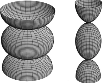
The immersion function is given by F⫽⌽⫺1␮(⳵⌽/⳵␭). In particular if␾⫽␯v, where␯is a real constant, q⫽q(u), then q(u) satisfies 共Fig. 1兲

quu⫽⫺2q3⫺␯q. 共92兲

Lemma 5.3: Let U,V,A,B be defined by Eqs. 共81兲, 共82兲, and 共84兲 where r⫽q(u)sin(␯v), s ⫽q(u)cos(␯v), ␭,␯,␮ are constants and q(u) satisfies 共92兲. Then the associated surface S is a Weingarten surface satisfying the relation

2␮2H2共␮2K⫺␯兲⫽共3␮2K⫹4␭2⫺2␯兲2. 共93兲 If␯⫽⫺4␭2 the above-mentioned Weingarten relation becomes quadratic,

K⫺2

9H

2_⫹4␭ 2

9␮2⫽0. 共94兲

(13)

VI. DEFORMATIONS OF THE MODIFIED KORTEWEG–DE VRIES SURFACES Let␳(u,v) satisfy the so-called modified Korteweg–de Vries共mKdV兲 equation

␳v⫽␳uuu⫹32␳

2_␳

u. 共95兲

The associated U and V matrices defining its Lax pair are given by

2 ⫹共␳u 2_⫹4␭2_␳2_兲dv2

册

_, _共103兲 ds_II2⫽ ␭␮ 共␳u 2_⫹4␭2_␳2_兲 1/2 关⫺␳2_du2_⫹共⫺2_␳␳ uu⫹␳u 2_⫹2␭2_␳2_⫺_␳4_{兲du dv⫹}1 4共⫺4␳␳uuuu⫹4␳u␳uuuu ⫹12␭2_␳␳ uu⫺8␳3␳uu⫺4␭2␳u 2_⫺6_␳2_␳ u 2_⫺4␭4_␳2_⫹4␭2_␳4_⫺_␳6_兲dv2_. _共104兲

(14)

The immersion function is given by F⫽⌽⫺1␮(⳵⌽/⳵␭). A particular reduction of the above-mentioned surface is a Weingarten surface with a complicated Weingarten relation.

Lemma 6.2: Let U, V be defined by Eqs.共96兲 and 共97兲 where ␭,␮,␣are constants and␳(u) satisfies

␳uu⫽␣␳⫺

␳3

2 . 共105兲

Then the associated surface S is a Weingarten surface satisfying the relation

␮2_H2_␳2_关4共_␣_⫹4␭2_兲⫺_␳2_兴3_⫽16␭2_关_␳4_⫺6_␳2_共_␣_⫹4␭2_兲⫺8␭2_共_␣_⫹4␭2_兲兴2_, _共106兲 where ␳2_⫽4共_␣_⫹4␭2_兲⫹16␭ 2 ␮

冑

␣⫹4␭2 K⫹4␭2/␮2. 共107兲 It is interesting that using a different Lax pair for Eq.共105兲 it is possible to obtain a Wein-garten surface simpler than the above:

Lemma 6.3: Let U, V be defined by

. 共111兲

The geometrical quantities of the surface S associated with these U,V,A,B are given by

K⫽ 2 ␮2关␳2⫺2␣兴, H⫽ 1 ␮␳关3␳2⫹2共␭2⫺␣兲兴, 共112兲 dsI 2_⫽␮ 2 4 关共du⫹共␣⫹2␭兲dv兲 2_⫹_␳2_d_v2_兴, _共113兲 ds_II2⫽␮␳ 2 关du⫹共␣⫹␭兲dv兴 2_⫹␮␳ 4 共␳ 2_⫺2_␣_兲dv2_. _共114兲

The immersion function is given by F⫽⌽⫺1␮(⳵⌽/⳵␭). This surface is a Weingarten surface satisfying the relation

(15)

In the special case␣⫽␭2, this relation becomes

2␮2H2⫽9关␮2K⫹4␭2兴. 共116兲

VII. INTEGRABLE SPHERICAL CURVES

Consider the motion of a curve on a sphere of radius 1/␭. Assume that␳u⫽0. Then, using the results of Proposition A.1 it follows that its motion is characterized by

␭ sin␪

cos2␪ ␪t⫹V2␪u

冊

⫹c0, V3⫽⫺ cos␪

␭ 共V2u⫹V1␪u兲, 共119兲 where c0 is an arbitrary constant.

Proof: Spherical curves can be parametrized by共118兲, since for spherical curves,41

冉

␳u ␳2_␶

冊

2 ⫹_␳12⫽ 1 ␭2. 共120兲

The last equation in共144兲 can be written as V3⫽⫺(V2u⫹V1␶)/␳, which is the second equation

共119兲. The first two equations in 共144兲 imply 共117兲 and the first equation of 共119兲. QED

An integrable motion of a spherical curve. The motion of the curve on a sphere of radius共1/␭兲

is characterized by Eqs.共117兲–共119兲, where V2is an arbitrary function. Hence each choice of this

function yields a spherical surface. Let the velocity component V2 of this curve be given by V2⫽⫺␭ cos␪共␪ucos␪兲u, 共121兲 and let c0⫽␭3, then␪evolves according to the integrable equation

␪t⫺␪ucos␪⳵u⫺1

冉

sin␪ 共cos␪兲2␪t

冊

⫹ 1 2共␪ucos␪兲 3_⫹cos_␪_关cos_␪_共_␪ ucos␪兲u兴u⫽0. 共122兲

It seems that Eq.共122兲 has not appeared before in the soliton literature. We note that in the small

␪ limit this equation reduces to the potential modified KdV equation.

We note that the motion of curves on a sphere was studied recently in Ref. 8 by demanding that the geodesic curvature of these curves is constant and equal to 1/␭. It can be shown that this requirement is equivalent to␳⫽1/␭, 共i.e.,␳u⫽0兲. Thus the integrable evolutions obtained in Ref. 8 coincide with the modified KdV hierarchy.

VIII. CURVES FROM SURFACES

Appendices A and B show that it is possible to construct surfaces from the motion of curves. It is also possible to associate a curve evolution with a given surface. For this purpose it is more suitable to introduce the Darboux frame on curves.40

(16)

Let S be an oriented regular surface and␣:I→S be a curve C parametrized by its arc length. At the point p⫽␣(s) consider the following three unit vectors, called the Darboux trihedron: T(s) is the tangent vector to C at p, n(s) is the normal vector to S at p, and b(s)⫽n(s) ⫻T(s). These vectors satisfy the Darboux equations

dT ds⫽␳gb⫹␳nn, 共123兲 db ds⫽⫺␳gT⫹␶gn, 共124兲 dn ds⫽⫺␳nT⫺␶gb, 共125兲

where␳g⫽␳g(s), ␳n⫽␳n(s), ␶g⫽␶g(s), s苸I. The geometrical meaning of these coefficients is the following: The scalar␶g⫽⫺dN/ds•b is called the geodesic torsion of the curve C. This curve is a line of curvature of S if and only if␶g⫽0.␳n and␳gare the normal and geodesic curvatures of C, respectively, at a point p苸S.

Let␳ be the curvature of␣(s) at p which is defined by dT/ds⫽␳N, and N be the principle normal to the curve at p. Using the first equation共123兲 in the Darboux equations 共123兲–共125兲 we find

␳2_⫽_␳g2_⫹ ␳n

2

. 共126兲

Since the tangent vector T to the curve C is common in both frames it is possible to pass from the

Frenet trihedron to the Darboux trihedron by a special local SO共3兲 transformation. Let T, b, n

define the Darboux trihedron and T, N, B denote the Frenet–Serret triad of orthogonal vectors. Then

n⫽sin␪N⫹cos␪B, b⫽cos␪N⫺sin␪B. 共127兲 This enables us to connect the torsion␶and curvature␳of the curve C to its geodesic torsion␶g, geodesic and normal curvatures␳g,␳n.

This transformation induces a local SU共2兲 gauge transformation on the Lax equations 共145兲: Letting⌽

⬘

⫽S⌽, we find

U

⬘

⫽SUS⫺1⫹S_uS⫺1, 共128兲

V

⬘

⫽SVS⫺1⫹S_vS⫺1. 共129兲 The matrix S is given as

S⫽ 1

&

冉

e⫺i␪/2 ⫺ei␪/2

e⫺i␪/2 ei␪/2

冊

. 共130兲

In what follows we given an example of how a curve motion can be identified from a given surface.

Proposition 8.1: Consider the surface described in Theorem 2.2 of Ref. 1. This surface is

associated with the motion of a curve with curvature and torsion given by

2, 共132兲

where t⫽v and a⫽ds/du. Here s denotes the arc length. The components V1, V2, and V3 of the

velocity of this curve are defined in terms of ␳ and ␶ by the differential equations 共A1兲. An orthogonal frame on this curve is

T⫽⳵F ⳵s⫽⫺i⌽

⫺1_␴

Comparing these equations with共A4兲, we find

U1 a ⫽␪s⫺␶, U2 a ⫽␳sin␪, U3 a ⫽␳sin␪. 共140兲

Eliminating␪, Eqs.共131兲 and 共132兲 follow. It is now possible to identify the geodesic curvature

␳g, the normal curvature␳n, and the geodesic torsion␶gof the curve C in terms of the parameters of S: ␳g⫽␳cos共␪兲⫽ U₃ a , 共141兲 ␳n⫽⫺␳sin共␪兲⫽ U1 a , 共142兲 ␶g⫽␪

⬘

⫺␶⫽ U1 a . 共143兲 ACKNOWLEDGMENTS

We are grateful to F. Finkel for his help with plotting the surfaces. This work is partially supported by TUBITAK, Turkish Academy of Sciences and EPSRC under Grant No. GG/J71885.

(18)

APPENDIX A: THE MOTION OF CURVES

Let u denote the arclength of a curve inR3. This curve can be uniquely characterized, within a rigid motion in R3, by its curvature and its torsion. This characterization is expressed by the classical Frenet–Serret equations which define the dependence of the associated frame on u.3–9

Proposition A.1: Let the scalar real functions ␳(u,t) and ␶(u,t), which are differentiable functions of u and t for every共u,t兲 in some neighborhood of R2, denote the curvature and torsion of a curve with arclength denoted by u. Let the real scalar functions Vj, which are differentiable functions of u and t for every共u,t兲 in some neighborhood of R2, denote the velocity of this curve. The motion of this curve is defined by

⳵␳ ⳵t⫺ ⳵V1 ⳵u ⫹V2␶⫽0, ⳵␶ ⳵t⫹ ⳵V3 ⳵u ⫺V2␳⫽0, ⳵V2 ⳵u ⫹V1␶⫹V3␳⫽0. 共A1兲

These equations are the compatibility conditions of the following equations for the SU共2兲 valued function⌽(u,t), ⳵⌽ ⳵u ⫽ i 2

冉

␶ ⫺␳ ⫺␳ ⫺␶

冊

⌽, ⳵⌽ ⳵t ⫽⫺ i 2

冉

V3 V1⫺iV2 V1⫹iV2 ⫺V3

冊

⌽. 共A2兲

Proof: Let xj, j⫽1,2,3, be a point on a curve in R3 whose arclength is denoted by u. This leads to

兺

j⫽1 3

冉

⳵xj ⳵u

冊

2 ⫽1.

The Serret–Frenet frame is a triad of orthonormal vectors, T, N, B, where T is the tangent vector, N is the principal normal unit vector, perpendicular to T which lies in the oscillating plane of the curve, and B is the binormal unit vector, perpendicular to both T and N. The components of these vectors satisfy the condition

T2_j⫹N2_j⫹B2_j⫽1, j⫽1,2,3, 共A3兲

and the classical Frenet–Serret equations

⳵ ⳵u

冉

T_j Nj Bj

冊

⫽

冉

0 ␳ 0 ⫺␳ 0 ⫺␶ 0 ␶ 0

冊

冊

冉

Tj N_j Bj

冊

, j⫽1,2,3. 共A5兲

Using the su共2兲 representation of so共3兲, these equations yield 共A2兲.

Proposition A.2: Let the complex valued functions␺(u,t,␭) and V(u,t,␭), be differentiable functions of u and t for every共u,t兲 in some neighborhood of R2. Assume that␺and V satisfy

␺t⫽Vu⫹i␴␺⫺i␭V, 共A6兲

(19)

␴u⫽ ⫺i

2 共V¯␺⫹V␺¯兲. 共A7兲

Equations共A6兲 and 共A7兲 are the compatibility conditions of the following equations for the SU共2兲 valued function⌽(u,t,␭):

⳵⌽ ⳵u ⫽ 1 2

冉

i␭ ␺ ⫺␺¯ _⫺i␭

冊

⌽, ⳵⌽ ⳵t ⫽ 1 2

冉

i␴ V V ¯ _⫺i␴

冊

⌽. 共A8兲

Equations共A6兲 and 共A7兲 describe the motion of a curve with␳⫽兩␺兩,␶⫽(arg␺)_u⫹␭. The velocity of this curve satisfies

V₁⫹iV₂⫽V exp关⫺i⳵_u⫺1␶⫺i␭u兴, V_3u⫽⫺␶_t⫹␴_u.

Proof: Substituting the relations

␺⫽␳ei⳵u⫺1␶⫹i␭u_, _V⫽共V₁⫹iV₂兲ei⳵u⫺1␶⫹i␭u_, 共A9兲

into Eqs. 共A6兲 and 共A7兲 we find 共A2兲 and

⳵u⫺1␶t⫽

V_2u⫹V₁␶

␳ ⫹␴, ␴u⫽V2␳, 共A10兲

where⳵_u⫺1 denotes integration with respect to u. Eliminating␴from these equations we find that the equation obtained from the equations in共A2兲 after eliminating V₃.

Example A.1:共Constant torsion兲 The motion of a curve of constant torsion␶⫽␭ is

character-ized by ␳t⫽⫺␭V2⫺ 1 ␭ 共⳵u 2_⫹_␳2_⫹_␳ u⳵u⫺1␳兲V2, 共A11兲

where the velocities V1 and V3 can be expressed in terms of V2 and␳by

V₁⫽⫺1

␭ 共V2u⫹␳⳵u⫺1共V2␳兲兲, V3⫽⳵u⫺1共V2␳兲. 共A12兲 Proof: If␶⫽␭ Eq. 共A2兲 becomes

␳␶⫽V1u⫺␭V2, V3u⫽V2␳, V1⫽⫺

1

␭ 共V2u⫹␳V3兲. 共A13兲

These equations yield Eq. 共A11兲.

APPENDIX B: INTEGRABLE CURVE MOTIONS

It is well known that there exist many curve evolutions which are integrable. We call a curve evolution integrable if the motion is defined in terms of an integrable PDE. Integrable evolutions of curves have been studied extensively in the recent literature3–8. It turns out that for particular velocities, the motion of curves is defined by certain integrable equations, which include the sine-Gordon, the modified Korteweg-de Vries, the nonlinear Schro¨dinger, and the Hirota equa-tions. An obvious approach for obtaining integrable curve evolutions is to choose the functions Vj in such a way that the nonlinear equations共A1兲关or 共A6兲 and 共A7兲兴 are independent of ␭.

Example B.1:共Integrable evolutions of curves with constant torsion ␶兲 The motion of curve

with constant ␶⫽␭ is characterized by Eqs. 共A11兲 and 共121兲. Let its velocity be specified as follows:

(20)

Case 1: If V1⫽0, V2⫽⫺ 1 ␭sin␪, V3⫽ 1 ␭cos␪, 共B1兲

then␳evolves according to the sine-Gordon equation,

␳⫽␪u, ␪ut⫽sin␪. 共B2兲 Case 2: If V₁⫽␳_uu⫹1 2␳ 3_⫺␭2_␳_, _V 2⫽⫺␭␳u, V3⫽⫺ 1 2␭␳ 2_⫹␭3_, _共B3兲

then␳evolves according to the modified KdV equation,

␳t⫽␳uuu⫹ 3 2␳ 2_␳ u. 共B4兲 Case 3: If␭⫽1 and V1⫽␳uu⫹12␳ 3_⫺_␳_, _V 2⫽⫺␳u, V3⫽⫺12␳ 2_⫹1, _共B5兲

then␳evolves according to the Painlave II equation

␳⫽t1/3_W_共_␰_兲, _␰_⫽u共t兲⫺1/3_, _W ␰␰⫹13␰W⫹ 1 2W 3_⫽C, _共B6兲 where C is a constant.

Example B.2:共Integrable curve evolutions associated with the NLS兲 Let V⫽i␺x⫺␭␺,␴⫽12兩␺兩

2_⫹␭2_, _共B7兲

in Eqs.共A7兲 and 共A8兲, then␺evolves according to the nonlinear Schro¨dinger equation,

␺t⫽i␺xx⫹

i

2␺兩␺兩

2_. _共B8兲

This describes the integrable curve motion with␳⫽兩␺兩,␶⫽⳵_uarg(␺)⫹␭.

1_{A. S. Fokas and I. M. Gelfand, ‘‘Surfaces on Lie groups, on Lie algebras and their integrability,’’ Commun. Math. Phys.}

177, 203共1996兲.

2

A. S. Fokas, L. M. Gelfand, F. Finkel, and Q. M. Liu, ‘‘A formula for constructing infinitely many surfaces on lie algebras and integrable equations,’’共unpublished兲.

3_{G. L. Lamb, J. Math. Phys. 18, 1654}_共1977兲. 4_{H. Hosimoto, J. Fluid Mech. 51, 477}_共1972兲. 5

K. Nakayama and M. Wadati, J. Phys. Soc. Jpn. 62, 473共1993兲.

6

M. Gu¨rses, Phys. Lett. A 241, 329共1998兲.

7_{R. E. Goldstein and D. M. Petrich, Phys. Rev. Lett. 67, 3203}_共1991兲. 8_{A. Doliwa and P. M. Santini, Phys. Lett. A 185, 373}_共1994兲.

9_{Q. M. Liu, ‘‘Generalized conditional symmetries, asymptotic integrability, and integrable surfaces,’’ Ph.D. thesis,}

Clark-son University, 1995.

10_{M. Gu¨rses and Y. Nutku, ‘‘New nonlinear evolution equations from surface theory,’’ J. Math. Phys. 22, 1393}_共1981兲. 11_{A. Sym, ‘‘Soliton Surfaces,’’ Lett. Nuovo Cimento Soc. Ital. Fis. 33, 394}_共1982兲.

12_{A. Sym, ‘‘Soliton Surfaces. II,’’ Lett. Nuovo Cimento Soc. Ital. Fis. 36, 307}_共1983兲. 13

A. Sym, ‘‘Soliton surfaces. III. Solvable nonlinearities with trivial geometry,’’ Lett. Nuovo Cimento Soc. Ital. Fis. 39, 193共1984兲; ‘‘Soliton surfaces. IV. Topological charge for ‘Nontopological’ Solitons,’’ 40, 225 共1984兲; ‘‘Soliton Sur-faces. V. Geometric theory of loop solitons,’’ 41, 33共1984兲; ‘‘Soliton surfaces. VI. Gauge invariance and final formu-lation of the approach,’’ 41, 353共1984兲.

14_{A. Sym, O. Ragnisco, D. Levi, and M. Brushi, ‘‘Soliton surfaces, VII. Relativistic string in external field: General}

integral and particular solutions,’’ Lett. Nuovo Cimento Soc. Ital. Fis. 44, 529共1985兲.

15_{A. I. Bobenko, ‘‘All constant mean curvature tori in}_R3_{, S}3_{, H}3_{in terms of theta functions,’’ Math. Ann. 290, 209}

(21)

16_{A. I. Bobenko, ‘‘Integrable surfaces’’}_{共Russian兲 Functional Anal. i Prilozhen. 24, 68–69 共1990兲; translation in Funct.}

Anal. Appl. 24, 227–228共1991兲; ‘‘Surfaces in terms of 2 by 2 matrices, old and new integrable cases,’’ in Harmonic

Maps and Integrable Systems, edited by A. P. Fordy and J. C. Wood, Aspects of Mathematics共Friedr. Vieweg and Sohn,

1994兲, pp. 83.

17_{H. C. Wente, ‘‘Twisted tori of constant mean curvature in} _R_*_{’’ in Seminar on New Results in Nonlinear Partial}

Differential Equations, edited by A. Tromba, Aspects of Mathematics, Vol. E10,共Friedr. Vieweg and Sohn, 1987兲, pp. 1–36.

18_{U. Pinkall and I. Sterling, Ann. Math. 130, 407}_共1989兲. 19

D. A. Korotkin, ‘‘On some integrable cases in surface theory,’’ J. Math. Sci. 94, 65共1999兲. 关Translation of Zapiski Nauchnykh Seminarov Sankt-Petersburgskogo Otdeleniya Matematicheskogo Institute im V. A. Steklova Rossiiskoi Akademii Nauk. 234,共1996兲兴.

20_{J. Tafel, ‘‘Surfaces in}_R3_{with prescribed curvature,’’ J. Geom. Phys. 17, 381}_共1995兲.

21_{D. Levi and A. Sym, ‘‘Integrable systems describing surfaces of nonconstant curvature,’’ Phys. Lett. A 149, 381}_共1990兲. 22_{A. Sym, ‘‘Soliton surfaces and their applications}_{共soliton geometry from spectral problems兲,’’ in Geometrical Aspects of}

the Einstein Equations and Integrable Systems关Lect. Notes Phys. 239 154 共1985兲兴.

23

G. Konopelchenko, ‘‘Induced surfaces and their integrable dynamics,’’ Stud. Appl. Math. 96, 9–51共1996兲; ‘‘Nets in R3, their integrable dynamics and the DS hierarchy,’’ Phys. Lett. A 183, 153共1993兲.

24

W. K. Schief, ‘‘On the geometry of an integrable 2⫹1 dimensional sine-Gordon system,’’ Proc. R. Soc. London, Ser. A

453, 1671共1997兲.

25_{J. Cieslinski, P. Goldstein, and A. Sym, ‘‘Isothermic surfaces in E}3 _{as soliton surfaces,’’ Phys. Lett. A 205, 37–43}

共1995兲.

26_{J. Cieslinski, ‘‘A generalized formula for integrable class of surfaces in Lie algebras,’’ J. Math. Phys. 38, 4255}_共1997兲. 27_{T. K. Milnor, ‘‘Surfaces in Minkowski 3-space on which H and K are linearly related,’’ Michigan Math. J. 30, 309}

共1983兲.

28

H. Wu, ‘‘Weingarten surfaces and nonlinear partial differential equations,’’ Ann. Global Anal. Geom. 11, 49共1993兲.

29

M. J. Ablowitz and H. Segur, Solitons and the Inverse Scattering Transform共SIAM, 1981兲.

30_{A. C. Newell, Solitons in Mathematics and Physics}_{共SIAM, 1985兲.}

31_{Important Developments in Soliton Theory, edited by A. S. Fokas and V. Zakharov}_{共Springer, Berlin, 1993兲.} 32_{P. D. Lax, Commun. Pure Appl. Math. 21, 467}_共1968兲.

33

H. Hopf, Differential Geometry in the Large关Lect. Notes Math. 100 1983‡.

34_{J. Spruck, ‘‘The elliptic sinh-Gordon equation and the construction of toroidal soap bubbles,’’ in Calculus of Variations}

and Partial Differential Equations, Proceedings, Toronto, 1986 edited by S. Heldebrandt, D. Kinderlehrer, M. Miranda

关Lect. Notes Math. 1340 273 1988兴.

35

H. C. Wente, Pac. J. Math. 121, 193共1986兲.

36

U. Abresch, J. Reine Angew. Math. 394, 169共1987兲.

37_{R. Walter, Geom. Dedicata 23, 187}_共1987兲.

38_{P. J. Olver, Applications of Lie Groups to Differential Equations}_{共Springer, Berlin, 1991兲.}

39_{I. M. Gel’fand and L. A. Dikii, Usp. Mat. Nauk 30, 67}_{共1975兲; A. S. Fokas, Stud. Appl. Math. 77, 253 共1987兲.} 40

M. P. Do Carmo, Differential Geometry of Curves and Surfaces共Prentice–Hall, Englewood Cliffs, NJ, 1976兲, p. 261.