Çağri Sağlam*, Agah Turan and Hamide Turan
Saddle-node bifurcations in an optimal growth
model with preferences for wealth habit
Abstract: This paper studies the dynamic implications of preferences for wealth habit in a one-sector optimal
growth model. We show that the dynamics may encounter saddle-node bifurcations with respect to the parameters of the preferences: the relative weight of wealth in utility and the degree of wealth habit. We ana-lytically provide the monotone comparative statics and the continuity of the critical capital stock with respect to the discount factor, the relative weight of wealth in utility and the degree of wealth habit.
Keywords: Wealth habit; Threshold dynamics; Saddle-node bifurcation. JEL Classification: O41; C61; D90.
*Corresponding author: Çağri Sağlam, Department of Economics, Bilkent University, Turkey, e-mail: [email protected] Agah Turan and Hamide Turan: Department of Economics, Bilkent University, Turkey
1 Introduction
To account for the development patterns that differ considerably among countries in the long run (see Quah 1996; Barro 1997), a variety of one-sector optimal growth models that incorporate wealth (capital per capita) in utility (e.g., Kurz 1968; Zou 1994; Roy 2010) have been presented. These models are characterized by the existence of a critical capital stock in the vicinity of which small differences lead to permanent differences in the optimal path.1 However, to what extent the existence and the behavior of the critical capital stock in such
a framework depend on the parameters of the preferences and the discount factor have been overlooked.2
This paper introduces preferences for wealth habit in an otherwise standard one-sector optimal growth model. Showing that the dynamics may encounter saddle-node bifurcations, it examines the monotonicity and the continuity of the critical capital stock with respect to the parameters of the preferences: the weight of wealth in utility and the degree of wealth habit. The degree of wealth habit serves as a self-assessed reser-vation or subsistence wealth level as the agent cannot handle a decrease in his wealth below this level (see Bakshi and Chen 1996). Such a formulation with preferences for wealth habit instead of absolute wealth enables to capture not only that wealth is more valuable than its implied consumption rewards, but also that the degree of complementarity between the current and the next period’s wealth gets stronger as the weight of wealth in utility increases.
The fact that the presence of wealth effects preserves the monotonicity of the optimal paths and may lead to threshold dynamics with multiple stationary states dates back to Kurz (1968). The monotonicity of the optimal path stems from the fact that the utility as a function of capital stocks or the reduced form utility function has the positive cross partial derivatives (see Benhabib and Nishimura 1985). Recall that this condition is also nec-essary for the existence of multiple steady states (see Benhabib, Majumdar, and Nishimura 1987). Belonging to such classes of models with positive cross partials, we show that the minor differences not only in the weight of wealth in utility but also in the degree of wealth habit lead to permanent differences in the optimal path. 1 Various optimal growth models with some degree of market imperfections based on technological external effects and increas-ing returns also exhibit threshold dynamics (e.g., Dechert and Nishimura 1983; Mitra and Ray 1984; Kamihigashi and Roy 2007; Akao, Kamihigashi, and Nishimura 2011).
2 Akao, Kamihigashi, and Nishimura (2011) analyzes the monotonicity and the continuity of the critical capital stock with respect to the discount factor in a Dechert and Nishimura (1983) framework.
Akao, Kamihigashi, and Nishimura (2011) shows that the critical capital stock of the Dechert and Nishimura (1983) model is a decreasing and continuous function of the discount factor so that a small change in the discount factor does not cause a sudden regime shift unless the economy is exactly at the critical capital stock. In this paper, we show the corresponding results in a standard optimal growth model aug-mented by wealth habit in utility.
The rest of the paper is organized as follows. Section 2 describes the model and provides the dynamic prop-erties of optimal paths. Section 3 investigates the qualitative implications of the wealth habit on the long run dynamics and presents the monotone comparative statics and the continuity of the critical capital stock. The numerical analysis provided in this section complements the theoretical results. Finally, Section 4 concludes.
2 Model
The model differs from the classic one-sector optimal growth model by the assumptions on the preferences of the agents. Considering that wealth is more valuable than its implied consumption rewards, we assume that the utility depends not only on current consumption but also on wealth habit at each period. The model is formalized as follows: { }, =0 =0 [ ( ) ( )] max t t t t t t c z t u c w z β η +∞ +∞
∑
+ (P) subject to ∀t, ct+kt+1 ≤ f(kt), ∀t, zt = kt+1−γkt, ∀t, ct ≥ 0, kt ≥ 0, zt ≥ 0, k0 ≥ 0, given,where ct is the consumption and kt is the capital stock in period t. zt refers to the relative change of wealth
with respect to the past level of wealth namely the wealth habit at that period. γkt serves as a self-assessed
reservation or subsistence wealth level as the agent cannot handle a decrease in his wealth below this level. η∈R measures the relative weight of wealth habit in utility, γ∈(0, 1) measures the degree of wealth habit + and β∈(0, 1) is the discount factor. We employ an additively separable one-period utility function between consumption and wealth habit not only for analytical convenience but also for being consistent with recent empirical findings.3
We make the following assumptions.
Assumption 1 :uR+→R is continuous, twice continuously differentiable, and satisfies u(0) = 0. Moreover, it is + strictly increasing, strictly concave and u′(0) = +∞.
Assumption 2 :w R+→R+ is continuously differentiable, strictly increasing, concave and satisfies w(0) = 0.
Assumption 3 :f R+→R+ is twice continuously differentiable, strictly increasing, strictly concave and satisfies
f(0) = 0. Moreover, f (0) 1
β
′ > and lim→+∞ ( ) 1.′ <
x f x
3 Compared to the multiplicative form, the separable form of the preferences is more consistent with the empirical findings on the behavior of the wealthy households since these preferences do not put any restrictions on either the substitutability or the comple-mentarity between consumption and wealth habit [see Francis (2009) for details about the functional form of the utility function].
Assumption 3 implies the existence of a maximum sustainable capital stock A k( ) max{ , },0 = k k0 where k is such that ( )f k k= and f(k) < k for all k k> . For any initial condition k0 ≥ 0, a sequence of capital stocks
k = (k0, k1, k2, …) is feasible from k0 if γkt ≤ kt+1 ≤ f(kt) for all t. A sequence of consumption c = (c0, c1, c2, …) is
feasible if there exists a k feasible from k0 such that 0 ≤ ct ≤ f(kt)−kt+1 for all t. The preliminary results are
sum-marized in the following proposition.
Proposition 1 (i) For any k0 ≥ 0, there exists a unique optimal path k. The associated optimal consumption path,
c is given by ct = f(kt)−kt+1, ∀t. (ii) If k0 > 0, every solution (k, c) to the optimal growth model satisfies ct > 0, kt > 0, ∀t.
Proof: It is standard. See e.g., Le Van and Dana (2003).
Let V denote the value function, i.e.,
{ }
}
1 1 1 0 =0 =0 1 0 ( ( ) ) ( ) max ( ) , ( ), 0, given . β η γ γ + +∞ + + +∞ + − + − = ∀ ≤ ≤ ≥∑
t t t t t t t k t t t t u f k k w k k V k t k k f k kUnder Assumptions 1–3, the value function V is non-negative, continuous, strictly increasing, strictly concave, differentiable and satisfies the Bellman equation (e.g., Duran and Le Van 2003):
V(k0) = max{ u (f(k0)−k) + ηw (k−γk0) + βV (k) | γk0 ≤ k ≤ f (k0) }. The optimal policy function :g R+→R is defined by:+
0 argmax 0 0 0 0
( )= k { ( ( ) )− +η ( −γ )+β ( )|γ ≤ ≤ ( )}.
g k u f k k w k k V k k k f k
We will now show that the Euler equation begins to hold after some finite period of time and that the optimal paths are globally monotonic.
Proposition 2 (i) Let k be the optimal path from k0 > 0. Then, there exists an integer T such that γkt < kt+1 < f(kt) for
all t ≥ T and we have the Euler equation:
1 1 1 2 1 2 1
, ( )t t ( t t) ( t ) t ( t ) ( t t ).
t T u f k k+ ηw k+ γk βu f k+ k f k+ + βηγw k+ γk+
∀ ≥ ′( − )− ′ − = ′( − ) ′ − ′ − (1)
(ii) Let k k 0> 0 and k be the optimal path from k Then we have: ,t0. ∀ k k t≥ t.
Proof: The proof follows from Duran and Le Van (2003). See Appendix for the details.
The monotonicity of the optimal path stems from the fact that the utility as a function of capital stocks or the reduced form utility function has the positive cross partial derivatives (see Benhabib and Nishimura 1985). Recall that this condition is also necessary for the existence of multiple steady states (see Benhabib, Majumdar, and Nishimura 1987). The presence of wealth effects in utility has already been shown to lead to multiplicity of steady states (see e.g., Kurz 1968). In such models where γ = 0 the emergence of multiplicities solely depend on the relative weight of absolute wealth in utility. However, in our model, the existence of multiple steady states depends on the interplay between the relative weight of wealth effect in utility and the degree of wealth habit.
2.1 Dynamic properties of the optimal paths
As a monotone real valued sequence will either diverge to infinity or converge to some real number, the fact that the optimal capital sequences are monotone proves to be crucial in analyzing the dynamic properties and the long-run behavior of our model.
Proposition 3 Assume f (0) 1 β
′ ≥ . Let k be an optimal path from k0 > 0. Then, k can neither converge to 0 nor
diverge to +∞.
Proof: See Appendix.
A point ks is an optimal steady state if ks = g(ks), so that the stationary sequence ks = (ks, ks, …, ks, …) solves
the problem .P Recall that in a concave problem the stationary solution of the Euler equation is optimal since the transversality condition is satisfied. Let the set of stationary solutions to the Euler equation (1) be defined as: (1 ) ((1 ) ) 1 >0: ( ) . ( ( ) ) w k E k f k u f k k η βγ γ β β − ′ − = ′ + ′ − =
It is clear that whenever f (0) 1, β
′ ≥ E will be a non-empty set.
We will now show that our model can support unique optimal steady state with global convergence and the multiplicity of optimal steady states with local convergence. Indeed, we will revisit the results that the presence of wealth effects in utility leads to the multiplicity of optimal steady states even under convex tech-nology (see e.g., Kurz 1968). However, our concern is to analyze how the critical capital stock behaves in response to the changes in the preference parameters and the discount factor which have been to a large extent left unexplored.
Case 1 (Global Convergence) Assume k0 > 0 and
1
(0) .
f
β
′ ≥ Consider the case where there exists a unique element
ks in E. By Proposition 3, we know that the optimal paths cannot converge to 0. Then, any optimal path converges
to the unique optimal steady state ks, irrespective of their initial state.
Recall that the model reduces to the classic optimal growth model (η = 0) with (γ = 1−δ) or without (γ = 0) irreversible investment in which f (0) 1
β
′ > is a necessary condition of the existence of a positive steady state implying global convergence (see Duran and Le Van 2003). However, the presence of wealth effects in utility leads to the multiplicity of the optimal steady states even under convex technology.
Proposition 4 Let ˆ,k k E ∈ be two consecutive steady states. Then, they cannot both be stable.
Proof: Assume on the contrary that ˆk and k are both stable. Without loss of generality, let ˆ< .k k Then, there
exists kˆ0∈( , )k kˆ such that g k converges to ˆ.( )ˆ0 k Similarly, there exists k 0∈( , )k kˆ such that g k con-( )0 verges to .k This implies the existence of a critical capital stock, kc∈( , ).k kˆ kc is then either a genuine critical point at which the optimal policy has a jump or an unstable stationary capital stock which also belongs to the set E. However, the former violates the fact that the optimal policy is continuous and the latter is in contradic-tion with that ˆk and k are two consecutive steady states.
Case 2 (Local Convergence) Assume k0 > 0 and f′(0)≥β1. Let kl = min{k:k∈E} and kh = max{k:k∈E} denote the
lowest and the highest steady states, respectively. Suppose that kh is unstable from the right. Given the existence
of a maximum sustainable capital stock, as any optimal path from k0 > kh has to converge to an optimal steady
state, there will be another steady state larger than kh, a contradiction. Hence, kh is stable from the right. It is
also impossible to have kl unstable from the left, since the optimal paths can not converge to 0. Together with
Proposition 4, these already imply the existence of a critical capital stock and the emergence of the threshold dynamics even under convex technology by means of the wealth habit.
It can easily be seen from Proposition 3 and the continuity of the optimal policy that the economy can constitute only an odd number of hyperbolic steady states. For the sake of simplicity, consider now that there
exist three hyperbolic optimal steady states, kl < km < kh. Proposition 3 implies that kl is stable from the left and kh is stable from the right. These two results, together with the continuity of the optimal policy, naively suggest the existence of a critical capital stock and the emergence of the threshold dynamics. Moreover, the critical capital stock is equal to the unstable optimal steady state km so that the optimal path from k0 < km con-verges to kl and the optimal path from k0 > km converges to kh.
However, there can also be an even number of solutions to the stationary Euler equation which would imply the existence of a non-hyperbolic steady state. Even in such a case, threshold dynamics will emerge. For the sake of simplicity, suppose that there are exactly two optimal steady states, xl and xh. This can occur only when the optimal policy has a tangency to 45° line either at xl or at xh in which case the critical capital stock will be either xl or xh, respectively. It is then clear that any small perturbation in one of the parameters would cause a qualitative change in the dynamic properties of the optimal policy leading to a saddle-node bifurcation.
3 Wealth habit and the long-run dynamics
In this section, we analyze the qualitative implications of the wealth habit on the long run dynamics of the model. In order to provide a better exposition of our analysis, we will specify the functional forms and show that our model actually encounters a saddle-node bifurcation:
1 1 ( ) (1 ) , ( ) , 1 ( ) , 1 f k Ak k c u c z w z α σ θ δ σ θ − − = + − = − = −
where {A, σ, θ, η} > 0, α∈(0, 1), δ∈(0, 1], and γ∈[0, 1]. Check that f, u, and w satisfy the assumption sets. The stationary Euler equation can then be recast as Ψ(k) = Φ where
1 1 ( ) ( ) [1 ], (1 )(1 ) . k Akα σkθ σ Akα θ Ψ δ β βδ αβ Φ η βγ γ − − − − − = − − + − = − −
Under these functional forms, we first state the sufficient condition under which the unique steady state exists.
Proposition 5 There exists a unique steady state if either θ ≥ ασ or .
( ) 1
σα θ αβ
σ θ δ β βδ
− ≤
− − +
Proof: To ensure the existence of a unique steady state, it is sufficient to show that Ψ(k) is non-decreasing.
We have 1 1 1 1 1 1 ( 1 ( 1 ))(( ) ( )) ( 1 ) ( ) ( ) . ( ) ( ) k A k Ak Ak Ak k Ak k Ak k θ α α α α α σ α σ β α δ σα θ δ σ θ α βα δ Ψ δ δ − − − − + + − + − − + + − − − ′ = + − −
Note that Ψ′(k) ≥ 0 whenever f ′(k) ≤ 1, i.e.,
1 1 . A k α α δ −
≥ Recall that any steady state satisfies f k( ) 1, β ′ < i.e., 1 1 . 1 A k αβ α β βδ − > − + Let 1 1 * 1 α αβ β βδ − = − +A k and 1 1 ** α α. δ − = A
k It is then sufficient to show that Ψ′(k) ≥ 0 when
k∈(k*, k**).
If θ < ασ then 1 1 ( ) < ( )A k ασ θ α σ θ δ − − −
so that k < k** is trivially satisfied. However, k > k* requires that
> , ( ) 1 ασ θ αβ σ θ δ β βδ − − − + a contradiction. If σ > θ ≥ ασ then 1 1 ( ) < 0< * ( ) A k ασ θ α k σ θ δ − − ≤ − contradicts with k > k*. If σ < θ then 1 1 ( ) > . ( )A k ασ θ α σ θ δ − − − To have k < k**, < ασ θ α σ θ −
− has to hold, contradicting with α < 1. We now show that there can be at most three steady states.
Proposition 6 There can be at most three solutions to the stationary Euler equation.
Proof: To find the number of solutions to the stationary Euler equation, we prove that there can be at most
two local extremum values of Ψ(k). Ψ′(k) = 0 implies that ρ1k2(α−1)+ρ 2kα−1+ρ3 = 0 where 2 1 2 3 ( 1 ( 1)), (1 (1 ))( ) ( 1), ( )(1 (1 )). ρ β α θ α σ ρ β δ θ σα β δα θ σ α ρ δ σ θ β δ = − + − = − − − + − + − = − − − A A A
This implies that Ψ(k) can have at most two local extremum values, one of which is local maximum and the other is local minimum. As Ψ(0) < Φ and ( )> ,Ψ k Φ Ψ(k) and Φ can intersect at most three points.
The following proposition shows that when there exists a non-hyperbolic steady state there can only be two steady states.
Proposition 7 Let k be an optimal path from k0 > 0. Assume f′(0)≥β1. If there exist a non-hyperbolic steady state then there can exactly be two steady states.
Proof: The Jacobian matrix is given by:
1 2 1 = J ΩJ J− where 2 1 1 1 1 1 1 2 1 2 1 1 1 (1 ) ((1 ) ) (1 )( ) , (1 ) ( (1 ) ) ((1 ) ) (1 ( )) , (1 ) α σ θ θ θ σ σ α θ θ θ σ β α α ∆ Ω ηθ γ βγΩ Ω γ βηγθ γ βσ∆ Ω ∆ β α α ∆ σ ηθ γ βγ Ω γ βηγθ γ βσ∆ Ω − − − − − − − − − − − − − − − − − − − − − − + − − − = − − − − − + − − − − = − − − A k k J k A k k J k
with Δ = (Akα−δk), and Ω = (Aαkα−1+1−δ).
Let λ1 and λ2 denote the eigenvalues of J. Note that λ1+λ2 = Ω+J2 > 0 and λ λ1 2=β1 >0. At a non-hyperbolic
steady state, we have λ1 λ2 1 1 β
a local extremum point of Ψ(k), note the following: If Ψ″(k) = 0 and Ψ′(k) = 0 as Ψ(0) < Φ and ( )Ψ k >Φ, Ψ(k) and Φ intersect only once. But we know that if there exists a unique steady state, it is a hyperbolic one so that Ψ″(k)≠0. Moreover, as Ψ(k) and Φ intersect at a local extremum of Ψ(k), there can exactly be two steady states.
3.1 Monotone comparative statics and the continuity of critical capital stock
In this section, we analyze the effects of β, η and γ on the steady states and the critical capital stock. Note that the optimal policy is implicitly dependent on β, η and γ. Hence, in order to facilitate our discussion below, we first make this β−, η− and γ− dependence explicit in the notation by writing g(k, β, η, γ), kl (β, η, γ), kc (β, η, γ) and kh (β, η, γ).
Proposition 8 (i) Let 0 0 1 . ( ) lim k f k β → =
′ The optimal policy, g(k, β, η, γ), is strictly increasing in β∈[β0, 1). (ii) Let ks be a hyperbolic steady state. Then ks is saddle path stable if and only if it is increasing in η.
(iii) Let ks be a hyperbolic steady state. When γ β θ γ β θ ,
β θβ β θβ
− −
> <
− − ks is saddle path stable if and only if it is
increasing (decreasing) in γ.
(iv) The optimal policy g(k, β, η, γ) is continuous in β, η and γ.
Proof: (i) Follows from Amir, Mirman, and Perkins (1991; Theorem 5.5.d).
(ii) From the linearization around the steady state, we have λ1+λ2 > 0 and λ λ1 2 1 . β = By setting 1 2 1 , λ βλ = it can be seen that 2 2 1 λ
βλ + is increasing in λ2 when λ2≥1 .β If ks is saddle path stable then 2
1 1 λ β β > > and hence 1 2 1 1 λ λ β
+ > + so that Ψ′(k) > 0. Since Φ is increasing in η, a saddle path stable steady state is increasing in η. Conversely, if a hyperbolic steady state is unstable then it is decreasing in η. First, note in such a case that both λ1 > 1 and λ2 > 1. Since λ λ1 2=β1 , we must have λ2<β1 . By solving the following problem:
2 2 2 1 1 1 , max λ β λ βλ < < + one can show that λ1 λ2 1 1
β
+ < + which implies Ψ′(k) < 0 so that the hyperbolic steady state which is unstable is decreasing in η.
(iii) Φ is increasing (decreasing) in γ when γ β θ γ β θ .
β θβ β θβ
− −
≥ <
− − The proof is the same as of (ii). (iv) See Le Van and Dana (2003), pp. 34–35.
Note that the effect of an increase in γ on the marginal utility of the future capital stock, kt+1 has two com-ponents. The first component is positive since an increase in the subsistence wealth level, γkt, triggers the desire to increase the future capital stock:
2 1 1 1 1 ( ( ( )t t ) ( t t)) ( ) 0. t t t t u f k k w k k w k k k k η γ η γ γ + + + + ∂ − + − =− − > ′′ ∂ ∂ (2)
The second component is negative since it will increase the effect of kt+1 on the next period’s subsistence level, γkt+1, and make it harder to obtain further utility from the change in kt+2 with respect to kt+1:
2 1 2 2 1 2 1 2 1 1 1 ( ( ( ) ) ( )) ( ) ( ) 0. t t t t t t t t t t u f k k w k k w k k w k k k k β βη γ βη γ βηγ γ γ + + + + + + + + + + ∂ − + − =− ′ − + − < ′′ ∂ ∂ (3)
As long as w is linear, the total effect of the degree of the wealth habit γ on the choice of the future capital stock becomes negative, hence the optimal policy is decreasing in γ. When w is strictly concave, the net effect of a change in γ on the behavior of the optimal policy is ambiguous. However, the behavior of the steady states in response to a change in γ can still be determined. Letting kt = kt+1 = kt+2 = k, the net change in the marginal
utility of kt+1 with respect to γ turns out to be ( ) [ ( )]. 1 w z η θ β γ β θβ γ ′ − + − − Note that if γ β θββ θ, − ≥ − the marginal utility of kt+1 at a stable steady state will increase with γ.
A similar analysis can be undertaken to see the effect of η on capital accumulation in the long-run. As we show in Proposition 8-(ii), the values of the stable steady states increase with η.
Corollary 1 Let 0 0 1 = . ( ) lim k f k β → ′
Then, kl (β, η, γ) and kh (β, η, γ) are strictly increasing, kc (β, η, γ) is strictly
decreasing in β∈[β0, 1) and η > 0. When >γ β θ γ< β θ ,
β θβ β θβ
− −
− − kl (β, η, γ) and kh (β, η, γ) are strictly increasing
(decreasing), kc (β, η, γ) is strictly decreasing (increasing) in γ. All of them are continuous in β∈[β0, 1), γ∈(0, 1)
and η > 0.
Proof: The proof follows from Proposition 8.
Akao, Kamihigashi, and Nishimura (2011) analyzes the monotonicity and the continuity of the critical capital stock in the discount factor in a Dechert and Nishimura (1983) framework. Dechert and Nishimura (1983) concentrates on the effects of non-convex technology on the long-run growth paths. In this paper, our focus is rather on the preference component and we analytically provide the monotone comparative statics and the continuity of the critical capital stock with respect to the discount factor, the relative weight of wealth habit in utility and the degree of wealth habit. The behavior of the critical capital stock with respect to these parameters is important in explaining the persistent differences in per capita capital stocks among countries since minor differences in the relative weight of wealth habit in utility and/or the degree of wealth habit lead to permanent differences in the optimal path.
In the next section, we provide a numerical example in order to illustrate the results presented above.
3.2 Numerical analysis
We will numerically illustrate an example showing how a small perturbation in η or γ changes the long run dynamics. In particular, we demonstrate the emergence of a saddle-node bifurcation with respect to these parameters. We consider the following set of fairly standard parameterization:
A = 1, α = 0.4, δ = 0.01, σ = 0.95, θ = 0.01, β = 0.94.
Setting γ = 0.75, we have multiplicity of steady states when η is between 0.0327486 and 0.0329705 which are the critical values for the emergence of a saddle-node bifurcation (see Figure 1). As long as η < 0.0327486, i.e., before the bifurcation occurs, there is only one steady state, kl, which is globally stable. As η increases, the steady state capital stock increases too. For η = 0.0327486, an additional steady state appears in addition to kl and the dynamics are now characterized by two steady states, kl < km where kl is locally stable and km is unstable in the sense that it is stable from right but unstable from left. The optimal policy is tangent to 45° line at km and the corresponding eigenvalue at km equals to unity indicating the possible emergence of a saddle-node bifurcation. When η slightly increases from its critical value 0.327486, the unstable steady state splits into one locally stable and one unstable steady state through a saddle-node bifurcation resulting in three steady states, kl (stable) < km (unstable) < kh (stable). The coexistence of these three steady states is preserved until η = 0.0329705.
As the value of η gets closer to the critical value 0.0329705, the lowest stable steady state and the unstable steady state approach one another and at the critical value they merge into a non-hyperbolic steady state
400 Bifurcation diagram kss 350 300 250 200 100 0.03275 0.03280 0.03285 0.03290 0.03295 0.03300 η 150
Figure 1 Bifurcation analysis for variations in η for a fixed value of γ.
400 Bifurcation diagram kss 350 300 250 200 100 0.749 0.750 0.751 0.752 γ 150
Figure 2 Bifurcation analysis for variations in γ for a fixed value of η.
through the reverse saddle node bifurcation. Slightly above this critical value of the saddle-node bifurcation, the non-hyperbolic steady state ceases to exist leaving only the stable steady state kh which is now globally stable. Further increases in η only affects the value of the stable steady state.
In sum, two types of the saddle-node bifurcations emerge. The difference lies in the following: In the first one, the saddle-node bifurcation is realized for the pair of steady states km and kh and in the second, it is for the pair of steady states kl and km. Moreover, in the first one, as η increases, coalescence of the steady states into a non-hyperbolic steady state is observed and in the second, the qualitative change is in the form of creat-ing a pair of stable and unstable steady states simultaneously from a non-hyperbolic steady state.
A similar analysis can be done for the variations in γ for a fixed value of η. The resulting bifurcation diagram is given in Figure 2. Note the reverse effect of γ on the values of the steady states compared to the effect of η: An increase in γ decreases the level of the steady state while an increase in η increases it.
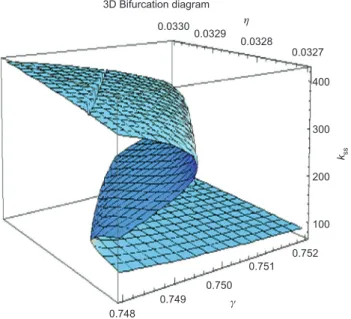
Figure 3 plots the steady states against the values of both the relative weight of wealth in utility, η, and the degree of wealth habit, γ. Note that the critical values of η specifying the region of the multiplicity shifts to the right as γ increases. This implies that the economies even with the same η and k0 can have different per capita capital stocks in the long-run depending on their degree of wealth habit.
4 Concluding remarks
In this paper, we analyze a model with multiple steady states in which utility depends on wealth habit rather than the absolute level of wealth in addition to consumption. We show that the dynamics may encounter saddle-node bifurcations with respect to the weight of wealth in utility and the degree of wealth habit so that minor differences in these parameters lead to permanent differences in the optimal path. We analytically provide the monotone comparative statics and the continuity of the critical capital stock with respect to the relative weight of wealth habit in utility, the degree of wealth habit and the discount factor.
Appendix
We prove Proposition 2 and Proposition 3 after providing some lemmas.
Lemma 1 Let k be an optimal path from k0 > 0. Then, there cannot be an integer T such that γkt = kt+1 for all t ≥ T.
Proof: Let k be an optimal path from k0 > 0. Assume that there exists such T. Since kt→0, under the
Assump-tion 3 there exists an integer T′ ≥ T such that βf k′( T′+1) 1.> The positivity of the optimal consumption implies that kt+1 < f(kt) for all t so that there exists ε > 0 small enough such that
3D Bifurcation diagram 0.749 0.750 0.751 0.752 100 200 300 kss 400 0.748 0.0330 0.0329 0.0328 0.0327 η γ Figure 3 Bifurcation analysis for variations in η and γ.
γkt < (1+ε)kt+1 ≤ f(kt), ∀t ≥ T′.
Define k as k k t= t for t = 1, …, T′ and k t= +(1 )ε kt for t ≥ T′+1. It is feasible as we have:
1 and 1 (1 ) 1 ( ) ( ), for 1.
t t t t t t
k k k k f k f k t T
γ = + + = +ε +≤ < ≥ ′+
Next, we show that k dominates k for some ε small enough. Define ( ) ( ) ( ).∆ ε =U k −U k By setting
ˆ( ) ( ) , f k f k= −γk we have: 1 1 1 > 1 ˆ ˆ ( )= [ ( ( ) ) ( ( ))] ( ) [ ( ((1 ) )) ( ( )] τ[ ( ((1 ) )) ( ( )] τ τ τ ∆ ε β γε β η γε β ε β ε ′ ′ ′ ′ ′ ′ +∞ ′+ ′+ ′+ ′+ − − + + + − +
∑
+ − T T T T T T T T T T u f k k u f k w k u f k u f k u f k u f kSince the second and the last terms are positive and u, f are concave and differentiable we get
1 1 ( )>[ ( ( )ˆ ) ( ( ))] [ ( ((1 )ˆ ˆ )) ( (ˆ )]. T T T T T T u f k k u f k u f k u f k ∆ ε γε β ε β ′ ′ − ′ − ′ + + ′+ − ′+ As ε→0, we have: 1 1 ( )> [ ( ( ))ˆ ( (ˆ )) (ˆ )]>0, T T T T T k u f k u f k f k ∆ ε γ β β ′ ′ − ′ ′ + ′ ′+ ′ ′+
which contradicts with the optimality of k.
Lemma 2 Let k be an optimal path from k0 > 0. Then, there exists an integer T such that γkt < kt+1 for all t ≥ T.
Proof: Let k be an optimal path from k0 > 0. Assume on the contrary that for any T there exists T′ ≥ T such that
1= .
T T
k k
γ ′− ′ Note that T′ can be chosen so that
1
<
T T
k k
γ ′ ′+ and βf k′( )>1T′ by Lemma 1 and by the fact that kt→0. The positivity of the optimal consumption implies that k f kT′< ( T′−1) for all t so that there is ε > 0 small enough to verify that
1 1
< ( ) and ( )< .
T T T T
k′+ε f k ′− γ k′+ε k ′+
Let k be a feasible sequence defined as
= for and = . t t T T k k t T≠ ′ k k ε ′ ′+ Let us define :∆R+→R by+ 1 1 1 ( )= ( (u f kT ) kT ) w( ) u f k( ( T ) kT ) w k( T (kT )). ∆ ε ′− − − +′ ε η ε +β ′+ −ε ′+ +βη ′+ −γ ′+ε
Differentiating Δ(ε) with respect to ε and evaluating at ε = 0, we obtain that
1 1
(0)> u f k( ( T ) kT ) u f k( ( T ) kT ) ( ) 0,f kT
∆′ − ′ ′− − − +′ ε β ′ ′+ −ε ′+ ′ ′ ≥
contradicting with the fact that Δ(ε) must have a maximum at ε = 0.
Lemma 3 Let k be an optimal path from k0 > 0. Then, there exists an integer T such that
ηw′ (kt+1−γkt)−βηγw′ (kt+2−γkt+1) ≥ 0, ∀t ≥ T.
Proof: Let k be an optimal path from k0 > 0. By Assumption 3, kt∈[0, A(k0)] for all t and by Proposition 2-(ii),
k is monotonic. Therefore, k must converge to some kss. Assume on the contrary that for any integer T there
exists τ ≥ T such that
As τ→+∞, we have
η(1−βγ)w′(δkss) > 0,
which contradicts with the continuity of w′.
Proof of Proposition 2
i) Assume that k0 > 0 and that k is optimal from k0. Proposition 1-(ii) establishes kt+1 < f(kt) for all t. Lemma 2
ensures that there is some T with γkt < kt+1 for all t ≥ T. This implies that constraints are not binding from time
T onwards, and hence the Euler equation begins to hold after T.
ii) Given k k k k0′> , 0 1′≥ 1 follows from Benhabib and Nishimura (1985). If k k′1= ,1 then *= *k kt′ t for t ≥ 1 as there is a unique optimal path associated to k1. By using this argument for t > 1, we can conclude that k kt′≥ t, ∀t.
Proof of Proposition 3
Let k be an optimal path from k0 > 0. Recall from Proposition 2 that the Euler equation implies
1 1 1 2 1 2 1
( ( )t t ) ( t t)= ( t ) t ( t ) ( t t )
u f k′ −k+ −ηw k′ +−γk βu f k′( + −k f k+) ′ + −βηγw k′ + −γk+
for all t ≥ T.
Assume first that k converges to 0. We have for all t ≥ T′:
u′(f(kt)−kt+1) > βu′(f(kt+1)−kt+2) f ′(kt+1) ≥ u′(f(kt+1)−kt+2)
where the first inequality follows from Lemma 3 and the second from the existence of some T′ ≥ T with βf ′(kt) ≥ 1 for all t ≥ T′. This implies that ct < ct+1 for all t ≥ T′. Since ct→0 as kt→0 we have a contradiction.
Assume now that k diverges to +∞. This violates the existence of a maximum sustainable capital stock.
References
Akao, K.-I., T. Kamihigashi, and K. Nishimura. 2011. “Monotonicity and Continuity of the Critical Capital Stock in the Dechert-Nishimura Model.” Journal of Mathematical Economics 47 (6): 677–682.
Amir, R., L. J. Mirman, and W. Perkins. 1991. “One-sector Nonclassical Optimal Growth: Optimality Conditions and Comparative Dynamics.” International Economic Review 32 (3): 625–644.
Bakshi, G., and Z. Chen. 1996. “The Spirit of Capitalism and Stock Market Prices.” American Economic Review 86: 133–157. Barro, R. J. 1997. Determinants of Economic Growth. Cambridge, MA: MIT Press.
Benhabib, J., and K. Nishimura. 1985. “Competitive Equilibrium Cycles.” Journal of Economic Theory 35: 284–306. Benhabib, J., M. Majumdar, and K. Nishimura. 1987. “Global Equilibrium Dynamics with Stationary Recursive Preferences.”
Journal of Economic Behavior and Organization 8: 429–452.
Dechert, W. D., and K. Nishimura. 1983. “A Complete Characterization of Optimal Growth Paths in an Aggregated Model with Non-concave Production Function.” Journal of Economic Theory 31: 332–354.
Duran, J., and C. Le Van. 2003. “Simple Proof of Existence of Equilibrium in a One-sector Growth Model with Bounded or Unbounded Returns from Below.” Macroeconomic Dynamics 7: 317–332.
Francis, J. L. 2009. “Wealth and the Capitalist Spirit.” Journal of macroeconomics 31 (3): 394–408.
Kamihigashi, T., and S. Roy. 2007. “A Nonsmooth, Nonconvex Model of Optimal Growth.” Journal of Economic Theory 132: 435–460. Kurz, M. 1968. “Optimal Economic Growth and Wealth Effects.” International Economic Review 9: 348–357.
Le Van, C., and R. A. Dana. 2003. Dynamic Programming in Economics. Boston: Kluwer Academic Publishers.
Mitra, H., and D. Ray. 1994. “Dynamic Optimization on Non-convex Feasible Set: Some General Results for Non-smooth Technologies.” Zeitschrift fur Nationaokonomie 44: 151–175.
Quah, D. T. 1996. “Convergence Empirics Across Economies with (some) Capital Mobility.” Journal of Economic Growth 1: 95–124. Roy, S. 2010. “On Sustained Economic Growth with Wealth Effects.” International Journal of Economic Theory 6: 29–45. Zou, H. 1994. “‘The Spirit of Capitalism’ and Long-run Growth.” European Journal of Political Economy 10: 279–293.