Joint routing, gateway selection, scheduling and power management optimization in wireless mesh networks

(1)

JOINT ROUTING, GATEWAY SELECTION,

SCHEDULING AND POWER MANAGEMENT

OPTIMIZATION IN WIRELESS MESH NETWORKS

A THESIS

SUBMITTED TO THE DEPARTMENT OF INDUSTRIAL

ENGINEERING

AND THE GRADUATE SCHOOL OF ENGINEERING AND

SCIENCE OF BILKENT UNIVERSITY

IN PARTIAL FULFILLMENT OF THE REQUIREMENTS

FOR THE DEGREE OF

MASTER OF SCIENCE

By Onur Uzunlar

(2)

ii

I certify that I have read this thesis and that in my opinion it is full adequate, in scope and in quality, as a dissertation for the degree of Master of Science.

___________________________________ Asst. Prof. Kağan Gökbayrak (Advisor)

___________________________________ Assoc. Prof. Emre Alper Yıldırım

______________________________________ Assoc. Prof. Ezhan KaraĢan

Approved for the Graduate School of Engineering and Science

____________________________________ Prof. Dr. Levent Onural

(3)

iii

ABSTRACT

JOINT ROUTING, GATEWAY SELECTION, SCHEDULING AND

POWER MANAGEMENT OPTIMIZATION IN

WIRELESS MESH NETWORKS

Onur Uzunlar

M.S. in Industrial Engineering Advisor: Asst. Prof. Kağan Gökbayrak

July, 2011

The third generation (3G) wireless communications technology delivers user traffic in a single step to the wired network via base station; therefore it requires all base stations to be connected to the wired network. On the other hand, in the fourth generation (4G) communication systems, it is planned to have the base stations set up so that they can deliver each other’s traffic to a small number of base stations equipped with wired connections. In order to improve system resiliency against failures, a mesh structure is preferred.

The most important issue in Wireless Mesh Networks (WMN) is that the signals that are simultaneously transmitted on the same frequency channel can interfere with each other to become incomprehensible at the receiver end. It is possible to operate the links at different times or at different frequencies, but this also lowers capacity usage.

In this thesis, we tackle the planning problems of WMN, using 802.16 (Wi-MAX) protocol, such as deploying a given number of gateway nodes along with operational

(4)

iv

problems such as routing, management of power used by nodes and scheduling while maximizing the minimum service level provided. The WMN under consideration has identical routers with fixed locations and the demand of each router is known. In order to be able to apply our results to real systems, we work with optimization models based on realistic assumptions such as physical interference and single path routing. We propose heuristic methods to obtain optimal or near optimal solutions in reasonable time. The models are applied to some cities in Istanbul and Ankara provinces.

(5)

v

ÖZET

ÇOKGEN BAĞLANTILI KABLOSUZ AĞLARDA ROTALAMA, AĞ

GEÇĠT DÜĞÜMÜ SEÇĠMĠ, ÇĠZELGELEME VE GÜÇ KONTROLÜ

PROBLEMĠNĠN BÜTÜNLEġĠK ENĠYĠLEMESĠ

Onur Uzunlar

Endüstri Mühendisliği Yüksek Lisans Tez Yöneticisi: Yrd. Doç. Dr. Kağan Gökbayrak

Temmuz, 2011

Üçüncü nesil (3G) kablosuz haberleĢme teknolojisi, kullanıcı trafiğini tek adımda baz istasyonu üzerinden kablolu Ģebekeye aldığı için bütün baz istasyonlarının kablolu Ģebekeye bağlı olmasını gerektirmektedir. Kurulum maliyetlerini düĢürmek için, dördüncü nesil (4G) kablosuz haberleĢme sistemlerinde her bir baz istasyonunun Ģebekeye kablo ile bağlanması yerine, birbirlerinin trafiğini Ģebekeye bağlı az sayıda baz istasyonuna ulaĢtırabilecek Ģekilde kurulmaları planlanmaktadır. Bozulmalara karĢı sistem direncini arttırmak için çokgen bağlantılı bir yapı tercih edilmektedir.

Çokgen Bağlantılı Kablosuz Ağlarda (ÇBKAlarda) karĢılaĢılan en önemli problem, aynı frekans kanalında ve aynı anda gönderilen sinyallerin ortamda fiziksel olarak birbirleriyle etkileĢime girerek alıcı tarafında anlamsız bir hal alabilmesidir. Bağlantıları farklı zamanlarda veya farklı kanallarda çalıĢtırarak etkileĢim

(6)

vi

önlenebilmekte ancak bu denetimin niteliği, kaynak kullanımındaki verimliliği de etkilemektedir.

Bu çalıĢmada, 802.16 protokolü kullanan ÇBKAlarda belirli sayıda ağ geçit düğümünün yerlerinin seçimi gibi planlama problemlerinin yanısıra, verilen en kötü hizmeti en iyileme amacıyla, bu seçimden kaynaklanan rotalama, düğümler tarafından kullanılan güç kontrolü ve çizelgeleme gibi operasyonel problemlere birlikte bakılmaktadır. Ele alınan ÇBKA, yerleri belirli ve trafik miktarları bilinen özdeĢ düğümlerden oluĢmaktadır. Sonuçların gerçek sistemlerde uygulanabilmesi için fiziksel etkileĢim ve tek rotalı eriĢim gibi gerçekçi eniyileme modelleri ile çalıĢılmaktadır. Daha kısa sürede ‘iyi’ sonuç elde etmek amacıyla bazı sezgisel yöntemler geliĢtirilmiĢ ve modeller Ġstanbul ve Ankara’daki bazı bölgelere uygulanmıĢtır.

Anahtar Kelimeler: Çokgen Bağlantılı Kablosuz Ağlar, Tamsayılı Programlama, Ağ Geçidi Seçimi

(7)

vii

Acknowledgement

I am sincerely grateful to Asst. Prof. Kağan Gökbayrak for his supervision, guidance, insights and supports. He has been supervising me with everlasting patience and interest from the beginning to the end. He was closer to me than a supervisor, ready to help whenever i needed him.

I also would like to express my deepest gratitude to Assoc. Prof. Emre Alper Yıldırım for his guidance and support throughout my study and his invaluable

feedback.

I would like to thank Assoc. Prof. Ezhan KaraĢan for accepting to read and review my thesis and for his invaluable suggestions.

I would like to acknowledge Mehmet Ünver and Selva ġelfun for their useful discussions and contributions to my work. I also would like to thank Gökhan Özçelik, Selva ġelfun, Hüsrev Aksüt, Ġsmail Erikçi and Muhammet Kolay for their

(8)

viii

I am grateful to my dear friends Fevzi Yılmaz, Pelin Elaldı, Müge Muhafız, Nurcan Bozkaya and Çağatay Karan for their invaluable camaraderie and helpfulness. My life became much easier with their support and motivation.

Last but not least, I would like to express my deepest gratitude to my family for their support, love, trust and motivation during my study.

Financial support of The Scientific and Technological Research Council of Turkey (TUBITAK) for the Graduate Study Scholarship Program is gratefully acknowledged.

(9)

ix

LIST OF FIGURES

Figure 1.1: Working Principle of a Mesh Router ... 2

Figure 1.2: A Typical WMN ... 3

Figure 1.3: Wired Transmission vs. Wireless Transmission ... 4

Figure 1.4: Interfering Signals ... 4

Figure 1.5: Illustration of TDMA Scheme ... 7

Figure 1.6: Frame Structure in TDMA ... 7

Figure 1.7: Illustration of FDMA Scheme ... 8

Figure 1.8: Illustration of OFDMA Scheme ... 8

Figure 2.1: Different Routing Methods ... 13

Figure 2.2: An Illustration of Clusters ... 14

Figure 3.1: An Illustration of Unnecessarily Added Constraints ... 26

Figure 4.1: Assigning Penalties ... 35

Figure 5.1: Placed Grid Topology on Kadıköy ... 38

Figure 5.2: Placed MRs on Kadıköy ... 38

Figure 5.3: Assigning Districts to the Placed MRs ... 39

Figure 6.1: Randomly Generated Topology ... 51

Figure 6.2: The Outcome of WMN 1 ... 52

Figure 6.3: The Outcome of WMN 2 ... 53

Figure A.1: The Network of KAD ... 59

Figure A.2: The Network of SAR ... 59

(12)

xii

Figure A.4: The Network of PEN ... 60

Figure A.5: The Network of USK ... 61

Figure A.6: The Network of CAN ... 61

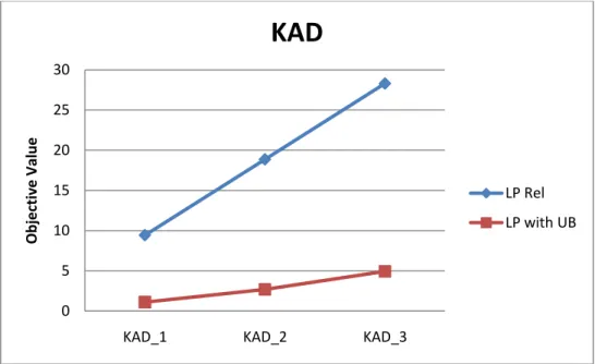
Figure C.1: LP Relaxation vs. LP Relaxation with Added Upperbound for KAD ... 63

Figure C.2: LP Relaxation vs. LP Relaxation with Added Upperbound for SAR ... 63

Figure C.3: LP Relaxation vs. LP Relaxation with Added Upperbound for PEN ... 64

Figure C.4: LP Relaxation vs. LP Relaxation with Added Upperbound for MAL ... 64

Figure C.5: LP Relaxation vs. LP Relaxation with Added Upperbound for USK ... 65

Figure C.6: LP Relaxation vs. LP Relaxation with Added Upperbound for CAN ... 65

Figure D.1: The Running Times of Each Model for KAD_1 ... 66

Figure D.4: The Overall Running Times of Each Model for KAD ... 67

Figure D.5: The Running Times of Each Model for SAR_1 ... 68

Figure D.8: The Overall Running Times of Each Model for SAR ... 69

Figure D.9: The Running Times of Each Model for PEN_1 ... 70

Figure D.12: The Overall Running Times of Each Model for PEN ... 71

Figure E.1: The Objective Value of KAD Using 5, 6 and 7 Transmission Slots ... 73

(13)

xiii

Figure E.3: The Objective Value of SAR Using 5,6 and 7 Transmission Slots ... 74

Figure E.4: The Objective Value of SAR Using 8, 9 and 10 Transmission Slots ... 75

Figure E.5: The Objective Value of PEN Using 5,6 and 7 Transmission Slots ... 76

Figure E.6: The Objective Value of PEN Using 8, 9 and 10 Transmission Slots ... 76

Figure E.7: The Objective Value of MAL Using 5,6 and 7 Transmission Slots ... 77

Figure E.8: The Objective Value of MAL Using 8,9 and 10 Transmission Slots ... 78

Figure E.9: The Objective Value of USK Using 5,6 and 7 Transmission Slots ... 79

Figure E.10: The Objective Value of USK Using 8,9 and 10 Transmission Slots ... 79

Figure E.11: The Objective Value of CAN Using 5,6 and 7 Transmission Slots ... 80

Figure E.12: The Objective Value of CAN Using 8,9 and 10 Transmission Slots ... 81

Figure F.1: 10th Node is Picked as the Gateway Node ... 82

Figure F.2: Transmissions Occuring in the First Transmission Slot ... 82

Figure F.3: Transmissions Occuring in the Second Transmission Slot ... 83

Figure F.4: Transmissions Occuring in the Third Transmission Slot ... 83

Figure F.5: Transmissions Occuring in the Fourth Transmission Slot ... 84

Figure F.6: Transmissions Occuring in the Fifth Transmission Slot ... 84

Figure F.7: Transmissions Occuring in the Sixth Transmission Slot ... 85

(14)

xiv

LIST OF TABLES

Table 3.1: Number of Variables and Constraints of WMN 1 ... 29

Table 3.2: The Names of the Relaxed Models ... 30

Table 5.1: The Parameters Used in the Numerical Examples ... 40

Table 5.2: Traffic Demands of Each Node Deployed in the Application Areas ... 41

Table 5.3: Solutions Obtained for KAD ... 42

Table 6.1: Number of Variables and Constraints of WMN 2 ... 50

Table 6.2: Comparison of WMN 1 and WMN 2 for the Randomly Generated Data ... 54

Table B.1: The Effect of Valid Inequality for MAL ... 62

Table D.1: Objective Value and Running Time of KAD ... 72

Table D.2: Objective Value and Running Time of SAR ... 74

Table D.3: Objective Value and Running Time of PEN ... 75

Table D.4: Objective Value and Running Time of MAL ... 77

Table D.5: Objective Value and Running Time of USK ... 78

Table D.6: Objective Value and Running Time of CAN ... 80

(15)

1

Chapter 1

Introduction

Wireless Networking Technologies are being used more frequently in recent years. After the Wireless Ad Hoc Networks, relatively new wireless technology, Wireless Mesh Networks (WMNs), have emerged as a cheap, easy to implement, efficient and reliable networking solution. As the number of users increased, the need for a better planned, faster, self-healing and flexible network also increased and WMNs propose an effective alternative for this need. Rather than delivering user traffic in a single step to the wired network, WMNs use a multi-hop structure to deliver user traffic. Hence, WMNs need less wired connection which decreases the deployment cost significantly. WMNs do not only lower the deployment cost but also lower the operational cost. It has been showed by M. Chee (2003) that using a mesh network to interconnect 133 existing hotspots in the Toronto downtown core will decrease the total cost of running hotspots by 70%.

(16)

2

A typical WMN consists of Mesh Clients (MCs), and Mesh Routers (MRs). A Mesh Client is actually a user, can be either mobile or stationary, trying to send/receive data to/from the Internet. Notebook users, smart phone users, PDA users are typical examples of MCs. MRs, on the other hand are static devices deployed in a deterministic way. Zhou et al., (2010) define MRs as powerful devices without constraints of energy, computing power, and memory and are usually distributed in a static and deterministic manner. Some of the MRs with special bridge functionalities, called gateways, play an important role within the WMNs. They connect WMNs to actual Internet with wire thus they are expensive to deploy.

Client C

Mesh Router Client A

Client B

Figure 1.1: Working Principle of a Mesh Router

The basic working principle of WMNs can be summarized as follows; as it can be seen in Figure 1.1, an MR gathers data from the MCs within its covering range and delivers it to the gateways. If the MR is within the Line-Of-Sight (LOS) transmission range of the gateway, the MR delivers its traffic through a single-hop link, however if the MR is not in the LOS transmission range, then it uses other MRs to reach the gateway and uses a multi-hop structure which increases the capacity usage in

(17)

non-3

LOS environments. According to Cao et al. (2006), the mesh topology not only extends the network coverage and increases capacity in non-LOS environments, but it also provides higher network reliability and availability when node or link failures occur, or when channel conditions are poor. A typical WMN can be seen in Figure 1.2.

INTERNET

Gateway Gateway

Mesh Router Mesh Router Mesh Router

Mesh Router Mesh Router Mesh Router Mesh Router

Figure 1.2: A Typical WMN

According to Akyildiz et al. (2004), WMNs have a wide range of application areas, including broadband home networking, community and neighborhood networking, enterprise networking, metropolitan area networks (MAN), transportation systems, building automation, military communications and surveillance systems etc.

In addition to all these advantages, WMNs have some issues. The major issue that drew the attention of researches is the Interference Problem. Different from wired networks, when a transmission occurs in a wireless network, signals trace a circular

(18)

4

pattern as shown in Figure 1.3. Since the transmission signals of the sender will also be received by other nodes within the transmission range, this situation will prevent them from receiving other signals. This is undesirable for wireless networks and the solution methods used to prevent interference decreases the network capacity significantly. A simple illustration of interfering signals can be seen in Figure 1.4.

Router A Router B

Mesh Router A Mesh Router B

Wired Transmission Wireless Transmission

Figure 1.3: Wired Transmission vs. Wireless Transmission

MR B MR A

MR C MR D

(19)

5

In Figure 1.4, MR B is in the transmission range of both MR A and MR C. The red and blue circles show the transmission signals of MR A and MR C, respectively. Suppose MR A is trying to send data to MR B and MR C is trying to send data to MR D at the same time, using the same frequency. MR B will not only receive the signals sent from MR A to itself but also the signals sent from MR C to MR D. Both of the signals will interfere with each other and become meaningless at the MR B and the transmission from MR A to MR B will fail and transmitted data will be lost.

In the literature, there are two main interference models; protocol model and physical model as defined by Gupta and Kumar (2000).

1. The Protocol Model: Suppose node i located at transmits over the bth subchannel to a node j located at . Then this transmission is successfully received by node j if

for every other node k simultaneously transmitting over the same subchannel. The quantity models the situation where a guard zone is specified by the protocol to prevent a neighboring node from transmitting on the same subchannel at the same time.

2. The Physical Model: Let S be the set of nodes that are simultaneously

transmitting at some time over a certain subchannel and let be the power level used by node i. Then the transmission between node i and node j is successful if

where is the corresponding signal-to-interference-noise-ratio (SINR), is the path loss exponent and is the ambient noise power level. Since the signal strength

(20)

6

between two nodes decreases as the distance between these nodes increases, we can calculate the loss between node i and node j, , as follows;

In the end, the physical interference model can be viewed as;

The physical interference model is much more realistic than the protocol interference model as it considers the effect of all other transmissions occurring simultaneously on the same subchannel. To successfully transmit the data, the MRs have to use enough power to reach beyond a certain threshold SINR value. Suppose node i transmits data to node j in a transmission slot and also there are some other transmissions occurring in the same transmission slot. For node j to successfully receive the data of i, the signal to interference ratio at the node j has to be over the certain threshold value. Thus for a successful transmission, the environment noise ratio and the effect of other ongoing transmissions in the same slot on node j should not be high to effect the quality of the transmission negatively.

Since, interference is the major issue, many schemes and channel access methods are proposed to carefully control the interference for multiple users while trying to use the available capacity efficiently. According to Kumar et al. (2006), these schemes can be classified into two: contention based and non-contention based. In the contention based schemes, no controller is needed and each terminal transmits data in a decentralized way. ALOHA and Carrier Sensing Multiple Access (CSMA) are typical examples of contention based schemes. In the non-contention based schemes on the other hand, a logic controller is needed. Time Division Multiple Access (TDMA), Frequency Division Multiple Access (FDMA) and Orthogonal Frequency Division Multiple Access (OFDMA) are among these multiple access schemes.

(21)

7

According to Garcia and Widjaja (2006), in TDMA, users all transmit using the same frequency and yet, their signals do not interfere with each others because different users transmit at different time slots as depicted in Figure 1.5. In TDMA, the time is divided into time slots that are assigned to the different users such that all users are using the same frequency band for transmission. Suppose there are N users sharing a single frequency band for transmission. In each slot, a user transmits data one after another and after the Nth user, the process is repeated again and again. The period in which all users are assigned one transmission time slot is called a frame, and it contains N time slots as shown in Figure 1.6.

time frequency

Figure 1.5: Illustration of TDMA Scheme

time U s e r 1 U s e r 2 U s e r 3 U s e r 1 U s e r 2 U s e r 3 U s e r N U s e r N

Frame 1

Frame 2

Figure 1.6: Frame Structure in TDMA

FDMA on the other hand, uses non-overlapping frequency bands for each user as depicted in Figure 1.7. Different than TDMA, users can transmit all the time.

(22)

8

time frequency

Figure 1.7: Illustration of FDMA Scheme

Finally, OFDMA which is a combination of both TDMA and FDMA divides the time into equal frames and allows transmissions using different frequencies as depicted in Figure 1.8.

time frequency

Figure 1.8: Illustration of OFDMA Scheme

In these schemes, only one transmission can occur in a certain transmission slot however spatial reuse allows more than one transmission to occur in the same transmission slot if the SINR threshold value for these transmissions is satisfied. By using spatial reuse, available capacity is used more efficiently.

There are protocols for wireless networking defined by Institute of Electrical and Electronics Engineering (IEEE) to control the operations like routing, media access control etc. These protocols are 802.11 Wireless Fidelity (Wi-Fi) and 802.16 Worldwide Interoperability for Microwave Access (Wi-Max).

(23)

9

802.11 protocol, which was originally defined for Wireless Local Area Network (WLAN), uses 2.4 GHz or 5 GHz unlicensed radio bands. 802.11a, 802.11b and 802.11g protocols are the most popular Wi-Fi protocols used. The data transmission rate for this technology differs between 11-54 Megabits per second (Mbps). The most common application areas of Wi-Fi are buildings, campuses, airports etc. Although 802.11 technology offers great advantages in terms of wireless networking, it is a decade old and was not designed for mesh networks (Djukic and Valaee, 2007)

802.16 Wi-MAX protocol on the other hand is designed for mesh technology and uses 2-11 GHz and 10-66 GHz radio bands. The 802.16, 802.16a and 802.16e are the most popular Wi-Max protocols. The original version of the standard was released in December 2001 and addressed systems operating in the 10-66 GHz frequency band. However, this system needed LOS environment which increases the deployment cost significantly. The 802.16a technology uses in 2-11 GHz band and operates in non-LOS environment. The data transmission rate can be increased up to 100 Mbps. Different than Wi-Fi, systems using Wi-MAX can be used to cover wider areas and the applications of the technology are cities, metropolitan regions etc.

In this thesis, we are jointly considering the Gateway Selection, Interference, Routing, Fairness, Scheduling, Power Management and Throughput problem of WMNs using 802.16 Wi-Max protocol. In our study Wi-MAX protocol is used since it offers great advantages in terms of providing next generation wireless networking solutions and has Metropolitan Area Network (MAN) applications.

In the literature, there are many studies addressing different problems in wireless mesh networks, however most of them do not consider these problems jointly. Since these problems affect each other, to provide an effective solution joint consideration of these aspects is crucial.

(24)

10

Using adjustable power level is also another contribution of the thesis. By controlling the power usage ratio in each transmission slot, more effective use of the network capacity is provided.

The remainder of the thesis is organized as follows:

In Chapter 2, considered problems will be outlined and relevant studies in the literature will be given. In Chapter 3, a Mixed Integer Linear Programming (MILP) model will be proposed to obtain exact solutions for the problems defined in the Chapter 2. The proposed model picks the predefined number of gateways among the placed MRs, finds a tree structured routing to the gateway nodes, assigns transmission slots to each MR and determines the power usage ratio of each node while maximizing the minimum service level. In Chapter 4, a special version of p-median problem is proposed to obtain ‘good’ solutions for larger networks in reasonable time. The heuristic will also be tested using numerical examples in terms of running time and quality. In Chapter 5, some real life applications will be given and the proposed system will be applied to some chosen areas in major cities of Turkey. In Chapter 6, some extensions will be provided and a MILP model which uses flexible path routing will be proposed. Finally in Chapter 7, we will conclude the thesis by briefly summarizing our efforts and contributions of the thesis. We will also present future research opportunities in this chapter.

(25)

11

Chapter 2

Problems in WMNs and

Problem Definition

2.1 Problems in WMNs

Although WMNs offers great advantages in terms of providing fast and reliable networking solution, WMNs have some deployment and operational problems. These problems of WMNs need a careful and logical planning. The major problems that drew the attention of researchers are Gateway Selection Problem, Routing Problem, Scheduling Problem, Covering Problem, Channel Assignment Problem, Clustering Problem, Fairness and Power Management Problem.

Gateway selection problem (GSP) is one of the most commonly studied problems of WMNs in the literature. It is the problem of determining the MRs with bridge functionalities among the placed ones. Different than a usual MR, gateways are much more expensive and complex devices. As they are connected to the actual network with wire, deployment of these devices are also costly. Since the gateway

(26)

12

selection affects the throughput, routing, scheduling and capacity usage; these aspects of WMNs should be jointly considered.

The GSP is shown to be NP hard by He et al. (2006) by using a reduction from the Capacitated Facility Location Problem (CFLP). In this study, a mixed integer linear program with two objectives is proposed. One objective is to use minimum number of gateways and the other objective is to use minimum number of hops for each MR to reach the gateway. Also, two heuristic approaches are proposed and the efficiency of heuristics is tested using simulation technique. However, in this study interference, which is the most challenging issue in WMNs, and scheduling are not considered.

Another research on Gateway Placement is done by Zhou et al. (2010). An innovative gateway placement scheme is proposed which considers the number of MRs, MCs and gateways. Protocol interference model is used and the throughput performance has been tried to be enhanced. Two throughput metrics are defined with this manner: maximizing aggregate throughput of WMNs and maximizing the worst-case-per client throughput in the WMN.

In addition, Routing Problem in WMNs is to find the paths that will carry the data packets to the selected gateway while considering the interference. There are also alternative methods used for routing MR traffic to the gateway. Using a tree structure rooted at gateway node, using multiple paths to carry data by dividing it and using flexible paths are among these methods. The Figure 1.5 depicts an illustration of these methods. In this figure, gateway node is depicted as black node with number 1. In the first picture, traffic division is not allowed and the final routing is a tree structure rooted at gateway. In the second picture, traffic division is allowed and data proportions follow different paths to reach the gateway. The traffic of 7th node is divided into two proportions. One proportion follows 7-4-2-1 to reach the gateway while other uses 7-8-9-5-3-1. Finally in the third picture, without allowing traffic

(27)

13

division, nodes are allowed to follow flexible paths. The 4th node gathers the data of 6th and 7th node. Although it sends the traffic of 7th node and itself by using 4-2-1, it is allowed to send the traffic of 6th node via another path, 4-5-3-1.

1 3 2 5 4 6 7 8 9 1 3 2 5 4 6 7 8 9 1 3 2 5 4 6 7 8 9

Tree Routing Multipath Routing Flexible Path Routing

Figure 2.1: Different Routing Methods

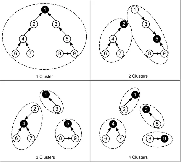
As mentioned before, routing the traffic of a node to a gateway also assigns the node to that gateway. If there are more than one gateway, then the MRs will be clustered so that each cluster has a gateway and MRs in each cluster are routed to that specific gateway. To satisfy the desired objective function, these clusters should also be formed in a logical manner. Figure 1.6 illustrates these clusters.

Aoun et al. (2006) have proposed an Integer Linear Programming (ILP) formulation to cluster MRs in such a way that the maximum number of hops in each cluster is bounded above by R while ensuring relay load and cluster size constraints. To cope with larger networks, an algorithm, based on recursively computing minimum Dominating Sets has been proposed. However, neither the traffic demand of each router nor the interference has been taken into account which are among the most crucial aspects of the WMNs.

(28)

14 1 3 2 5 4 6 7 8 9 1 3 2 5 4 6 7 8 9 1 3 2 5 4 6 7 8 9 1 3 2 5 4 6 7 8 9 1 Cluster 2 Clusters 3 Clusters 4 Clusters

Figure 2.2: An Illustration of Clusters

Locating the MRs to cover all the MCs is also another problem in WMNs. Since an MR can cover all the MCs within its transmission range, MRs should be located in a logical manner to cover the MCs and provide service.

Channel assignment problem is also an issue for radios using multiple channels. Determining which transmission to use which channel while considering interference has also been another hot topic for researchers.

Although power consumption is not a significant problem for WMNs, as the power used by MRs affect both the transmission rate and the interference caused on other

(29)

15

nodes, it is also quite crucial to determine power levels used by MRs. Power levels should not only be adjusted to provide connectivity within the network, but also transmit minimum interference to the environment. If the power levels are too low, this will cause a disconnected network, whereas if they are too high, this will cause extra interference to the environment and prevent effective capacity usage. The problem of determining the minimum range between two nodes for a disk area of A with n nodes is studied by Gupta and Kumar (1998). This study is further developed by Kawadia et al. (2001) and an algorithm is proposed to find minimum power level for a connected graph.

Delivering the MCs a fair service is yet another aspect of WMNs. One cannot let a certain MR use the whole capacity while restricting others. Thus, defining a fairness criterion and trying to satisfy it is quite crucial. According to Pioro et al. (2004), an intuitive way to approach this problem is to assign as much volume as possible to each demand, at the same time keeping the assigned volumes as equal as possible. This intuitive requirement leads to the assignment principle called Max-Min Fairness (MMF), known also as equity or justice in other applications. In our problem, we are using the same criterion and trying to maximize the minimum provided service level to each MR.

In our problem, similar to Cao et al. (2006) we have focused on the centralized scheduling of the IEEE 802.16 mesh mode, where a scheduling tree rooted at the gateway node is constructed for the routing path between each MR and the gateway, and the gateway acts as the centralized scheduler that determines the transmission or reception of every MR in each minislot.

(30)

16

2.2 Problem Definition

In our problem, we are given the number and the locations of mesh routers, and our aim is to maximize minimum service level using a predefined number of gateways and to use the available capacity as much as possible.

Each mesh router gathers data from the mesh clients within its transmission range and tries to deliver gathered data to the mesh routers with gateway functionalities to reach the Internet. In this problem, only uplink traffic (from MRs to the Internet) is considered. It is supposed that each router is equipped with two radio interfaces and one radio is used to control the local traffic (from MCs to MRs) while the other one is used to control the backbone traffic (among MCs) as in Zhou et al. (2010). Since we are not dealing with the local traffic, we assume each MC is served by the closest MR.

As only one radio is used for the transmissions between two MRs, a node can only transmit or receive in a single slot and cannot do both simultaneously. Transmission between two MRs occurs if the SINR threshold for communication is satisfied. As the location of each MR is known, one can easily determine the propagation loss between each node pair. This determination helps us to understand whether a node pair can communicate with each other or not.

Traffic division is not allowed in our problem as it creates some problems for the users. Especially for the Voice-Over-IP (VoIP) applications, receiving data simultaneously is a quite significant performance measure. In case of traffic division, the variation of arrival intervals for each packet may vary causing some problems for the user. Thus, traffic division is not allowed.

The network under consideration consists of nodes and arcs. Each MR is represented by the nodes in the network with predefined locations. As mentioned before, these

(31)

17

MRs are static and each has demands to be delivered to the gateway node. Transmissions between two nodes are represented by edges. Suppose node i can transmit data with a maximum power defined by and the propagation loss between node i and node j is defined by . There exists an arc between node i and node j if where is the SINR threshold value. For simplicity, we

define .

As mentioned before, maximizing the minimum service level is one of the most crucial aspects of our study. We define a service ratio and aim to satisfy all the MRs with the same service ratio to provide fairness among MRs. Suppose is the amount of flow that node i has to deliver to the gateway node and m is the ratio defined as minimum capacity allocated to node i / the demand of node i. In this study, is the minimum capacity allocated to node i. Our aim is to provide a service to all customers while maximizing the defined service level.

The most related work to our study is proposed by Targon et al. (2010) which is an extension of the GSP including joint routing and scheduling aspects. Similar to our assumption, traffic division is not allowed in this study. An ILP formulation is presented which tries to minimize gateway deployment cost. The model finds the location of the gateway nodes along with routes from each MR to the found gateways and a schedule for each MR. Although most of our assumptions are similar to those, our model is an extended version of this study. Rather than trying to find a schedule and routing for the given traffic demands of each MR, we are trying to provide a service level to each MR and trying to maximize the minimum service level. Also, in our study we have power control option so that transmitting MRs can adjust their power level to increase the use of the available capacity. In addition, we use physical interference model which is more realistic than the interference model used in this study. Rather than trying to deploy a given number of gateways, this study involves with finding minimum gateway deployment cost to provide service.

(32)

18

Chapter 3

Model Formulation

In this chapter, we will formulate a Mixed Integer Linear Programs (MILP) to solve joint scheduling, routing, gateway selection and power control problem, using physical interference model in OFDMA based single rate wireless mesh networks while maximizing minimum service level provided.

In the first part of the chapter, we will define the model , which uses the tree-routed structure and then add some valid inequalities and upper bounds to improve the running time of the model.

(33)

19

3.1. MILP Formulation

3.1.1 Assumptions

The assumptions listed below are used to model the problem defined earlier

 WMN under consideration uses 802.16 Wi-MAX standards

 OFDMA is used as multiple access scheme

 There is a finite number of MRs operating

 All the MRs used are identical

 All the locations of these MRs are known

 Multi rate transmission is not allowed

 Each MR is equipped with two radio interfaces

o One for the local communications (among MCs and MRs) o One for backbone communications (among MRs)

 Traffic division is not allowed

 Tree-routed structure allowed

 Each MC is served by the closest MR

 Omni-directional antennas are used

 Ambient noise power is static

3.1.2 Sets and Parameters

To model the problem, following sets and parameters are used;

- N denotes the set of Nodes i.e. MRs where

- A denotes the set of Arcs i.e. available transmissions. We can say that the directed link if and the propagation loss is calculated as follows;

(34)

20

where is the path loss exponent and is the distance between node i and node j.

-T denotes the number of non-interfering transmission slots. This can be either transmissions being active in different time slots or transmissions using non-interfering frequencies in the same slot.

-c denotes the capacity of an existing link. If two nodes can communicate with each other, than they can send data with a rate defined as c.

-G denotes the number of gateways to be deployed.

- denotes the capacity vector of a gateway. If a gateway is placed at a node, then it will have a capacity equal to .

- denotes the traffic vector of the MRs in the WMN. A node i collects the traffic of all MCs within its coverage range and tries to deliver it to a gateway.

- denotes the signal strength of node i at node j while node i transmits data using maximum power available.

- denotes the noise value in the environment.

- denotes the corresponding SINR threshold value required for a successful transmission

(35)

21

3.1.3 Mixed Integer Linear Programming Model

3.1.3.1 Variables

The following variables are needed to model the problem.

3.1.3.2 Formulation of MILP

The following MILP, WMN1, is constructed to solve the problem defined earlier. The model jointly considers the gateway location, scheduling, routing and power control aspects of the problem using a tree routing structure. The aim is to maximize the minimum service level provided to each customer and use the capacity of the network efficiently.

(36)

22

(37)

23

Our objective is to maximize the minimum service level provided to all customers while ensuring the constraints.

Constraint is the capacity constraint. If a link is active in a period t then it has available capacity to transmit the data in this period. Thus, the traffic flow on a link cannot be more than the available capacity.

Constraint ensures that the actual traffic given to the system by node i equals to the provided service level times the traffic of that node. Similarly, constraint is added to make sure that the amount of traffic flow using node i as gateway cannot be larger than the gateway capacity of that node. Constraint implies that the total number of gateways to be deployed is equal to .

is the flow conversation constraint. The traffic flow from other nodes reaching node i and the traffic flow of node i equals to the leaving traffic flow from node i. Constraint ensures that the traffic of each node has to follow a single route to reach the gateway.

Constraint implies that there can be a transmission between node i and node j if and only if the link under consideration is used. Since each MR is equipped with a single radio used for transmission, then in a single transmission slot, it can only send or receive data and it cannot do them simultaneously. The single radio issue is handled by .

Constraint is the power usage constraint. The power ratio used by node i in period t cannot be larger than 1.

The most crucial and restrictive constraint of the model is the interference constraint. As mentioned earlier, different than most of the studies, a more realistic physical

(38)

24

interference model is used in our model. Constraint is the physical interference constraint.

Non-linear constraint , is linearized as follows;

where is a sufficiently large, positive number.

For the linearized constraint , if , then this means node i transmits data to node j in transmission slot t and the constraint becomes;

which means the minimum SINR value for this

transmission have to be greater than plus any other transmissions occurring in this time slot t.

If there is no transmission from node i to node j, i.e. , then the constraint becomes; which becomes redundant because

of the choice of .

used in this constraint is calculated as follows;

which is always greater than the right hand side (RHS) of the constraint to make it redundant when .

Finally, the constraints and imply that these variables are binary and similarly and are added to define positive variables.

(39)

25 In the end becomes;

.

3.1.3.3 Additional Constraints for WMN1

The following additional constraints are added to the WMN1 to narrow down the solution space and help the solver find the optimal solution faster, without changing the final solution. These kinds of inequalities are called as valid inequalities. According to Cornuejols (2006), an inequality is said to be valid for a set if it is satisfied by every point in this set and a cut with respect to a point is a valid inequality for that is violated by where is the convex hull of S.

Although the valid inequalities may narrow down the solution space, they do not always improve the running time of the solver. There is a tradeoff between adding valid inequalities and the number of constraints. As the number of valid inequalities increases, the solution space will narrow down however as the number of constraints increases, the model will contain too many constraints which may cause clumsiness in terms of the running time of the model. An illustration of unnecessarily added valid constraints is given in Figure 3.1.

In the figure below, ABCD defines a polyhedra and the red point is the optimal integer solution. The valid inequalities are added and they narrowed the solution space down, however they do not cut off the fractional solutions around the optimal solution and thus do not help the solver with the running time. Adversely, they may increase the number of constraints and may increase the running time of the model.

(40)

26

A

B C

D

Figure 3.1: An Illustration of Unnecessarily Added Constraints

Proposition 1. The following inequality is valid for the polyhedra defined by the

constraints of WMN1.

Proof. Suppose , which means that the link is used for transmission. Then becomes which implies the link has to be active in at least one of the transmission slots which is what we desire.

Similarly, suppose . Then becomes which is valid because the constraint forces no link to be active in any of the transmission slots. Thus , implies. Hence the constraint is valid for the polyhedra defined by the constraints of

(41)

27

The effect of the added valid inequality can be seen in Appendix B.

3.1.3.4 Improving the Upper Bound of WMN1

In addition to the added constraints, adding some lower and upper bounds on the objective value may improve the running time of the solver. The basic working principle of a typical MILP solver can be summarized as follows; the solver tries to find feasible solutions using heuristic methods. For a maximization problem, each feasible solution found is a lower bound on the objective value and conversely, the relaxation of the model yields an upper bound on the objective value. The solver terminates when the upper bound and the lower bound get the same value.

With this point of view the following upper bounds are added to the model;

Proposition 2. The following inequality is an upper bound on the objective value,

, of the WMN1.

Proof. The constraint uses the available gateway capacity as an upper bound on the provided service level. Since each MR is provided with the same service level m, and all the traffic uses the gateways to reach the Internet.

Suppose is not an upper bound on , i.e.

, then the total throughput of the system is . However, since the throughput is bigger than the total gateway capacity, , such an is not feasible for the system, Thus is an upper bound for the optimal value of WMN1.

(42)

28

Proposition 3. The following inequality is an upper bound on the objective value,

, of the WMN1.

where and such that

.

Proof. The constraint uses the available link capacity as an upper bound on the provided service level. Since , and the traffic of the nodes with gateway functionalities will directly reach the Internet without using any links, then the traffic to be transmitted is . The available link capacity for the transmission of these data is at most . In each transmission slot, the links have available capacity. Since all the MRs have single radio, a gateway can only receive data from one node in a transmission slot, the maximum number of transmissions that a gateway can have equal to . Thus, for a gateway the maximum link capacity is and since there are gateways, the total available link capacity to transmit data is .

Thus, because of the link capacity constraint, the service level provided can be at

most;

even the traffic division is allowed. Since we do not know

which nodes will be chosen as gateway nodes, we can write;

Since , then and the

(43)

29

After adding the valid inequalities and constraints on the objective value, WMN1 becomes;

.

The effect of these bounds on the objective value is shown in the Appendix C by using LP relaxation.

In the end, the number of variables and constraints that has is listed in the following table.

# of binary variables # of other variables #of constraints

N+A(T+1) N(T+2)+A+1 N(2T+4)+A(2T+2)+3

Table 3.1: Number of Variables and Constraints of

In addition to adding valid inequalities and improving the upper bound, we needed to relax some binary variables and try to figure out the effects of these relaxations in the remaining part of the chapter.

(44)

30

3.2 LP Relaxation

has three sets of binary variables and . By relaxing each combination of these sets, we get following sub models shown in Table 3.2.

MODEL EXPLANATION

WMN1 None of the variables are relaxed

WMN1_x relaxed, and are binary

WMN1_y relaxed, and are binary

WMN1_z _relaxed,_and are binary

WMN1_xy _and_{are relaxed,} binary

WMN1_xz and are relaxed, binary

WMN1_yz and are relaxed, binary

WMN1_xyz All the variables are relaxed

Table 3.2: The Names of the Relaxed Models

After running the models separately, we see that and yield the same solution even though some of the binary variables are relaxed. In spite of relaxing the variables, the constraints on the model still forces them to get binary values. A comparison of these models is given in the Appendix D in terms of running time. According to that comparison, performs better in terms of running time than the others thus it is used in this study to solve the defined problem. From now on, whenever we say , this means we are using .

It is also seen that both and yield the same solution. Even though we additionally relax in , the constraints force it to have binary values. In these models, as is relaxed, the interference constraint no longer works.

(45)

31

Although interference is not considered by these models, an advantage of these models is that, they pick the gateways and determine the single routes from each MR to these gateways.

, on the other hand, picks a gateway and allows multipath routing without considering the interference. Since the constraint is found by the same manner, there is no doubt that the solution of will be equal to

.

Since the model, has too many binary variables, it takes excessive amount of time to obtain the optimal solution as the network size increases. Thus, we needed to devise some solution methods to obtain ‘good’ solutions in reasonable time for larger networks. The running time and the objective value of each run can be seen in Appendix E.

(46)

32

Chapter 4

Solution Methods

In this chapter, we will define some basic methods to solve the problem defined in Chapter 2, for larger networks. Since the problem we are dealing with is a joint consideration of more than one NP hard problem, the running time of the solver increases exponentially as the input size increases.

In our study, we have seen that pre-defining the gateway nodes for the WMN, decreases the running time as it cuts off the feasible solution space. However, we may lose the chance of finding the optimal solution. So, there is a tradeoff between obtaining a solution in reasonable time by defining the gateways and finding the optimal solution in excessive amount of time.

With this manner, we have tried to determine the gateway node in a logical manner to obtain a near-optimal solution in reasonable time. The problem is simplified by reformulating it as a special case of p-median problem and some additional

(47)

33

constraints are added. Then the solution of this formulation is used in to obtain a solution in reasonable time.

4.1 Heuristic Approach

The p-median problem, defined by Hakimi (1964), consists of locating p facilities on a network, so that the sum of the shortest demand weighted distances from each of the nodes to its nearest facility is minimized. When we start considering the capacities of the facilities, the p-median problem becomes the capacitated p-median problem (CPMP) which is defined by Maniezzo et al. (1998) and can be modeled as:

where is the distance from node i to node j, is the number of facilities to be

deployed, is the demand of node i and finally is the capacity of a facility. The binary variable equals to 1 if the demand of node i is satisfied by facility j and 0 otherwise.

(48)

34

Constraint implies that every node will be assigned to a facility. implies that the number of facilities to be opened is exactly v. Constraint on the other hand is the capacity constraint. The demands assigned to a facility cannot be larger than the capacity of that facility.

By making the following changes we can easily get a solution for our problem:

We also add following constraints to and obtain . The additional constraints are;

where is the link capacity and is the hop count value.

Constraint ensures that the total demand assigned to a gateway node cannot be larger than the total link capacity and implies that the number of hops that each MR uses is bounded by . In this approach, is the minimum number that satisfies a feasible assignment for the .

By solving , we are trying to give weighted penalties to each node. The penalty given to a node can be calculated as number of nodes traversed times the traffic demand of that node which is as shown in Figure 4.1.

(49)

35 1 3 2 4 5 6

Figure 4.1: Assigning penalties

In the figure above, 6th node is the gateway node and the traffic of node 1 is carried along the path (1-2-4-6) where it uses 3 hops to reach the gateway. Thus the penalty of node 1 is where is the traffic demand of the 1st node. The overall penalty of the system above is . Since we want to minimize the total penalty for all nodes, we are using the objective function of and trying to find the deployment with minimum penalty. The model tends to pick nodes with high traffic demands as gateway nodes.

In the latter case, we solve the by fixing the gateways found by . To easily express;

Heuristic

 Step 1. Solve and obtain the gateway set

 Step 2. Solve by fixing the gateway set found in the step 1.

In Appendix G, our heuristic is compared with the heuristic approach proposed by Zhou et al. and a basic approach defined as picking the nodes with highest traffic demand as gateway nodes. The red colored lines show that the chosen heuristic performs better than the others.

(50)

36

where and are the number of mesh routers and the number of gateways in the network, respectively. For each node in the system, Multihop Traffic-Flow Weight (MTW) is calculated as: .

Then the node with maximum value is picked as the gateway node. If there are more than one gateway to be deployed, some adjustment on the traffic demand of the routers are needed.

Another heuristic used to compare our approach is Busiest Router Placement (BRP) which consists of picking the nodes with highest traffic demand values as the gateway nodes.

In Appendix G, the outlined heuristics will be compared using the largest network we have.

(51)

37

Chapter 5

Numerical Examples

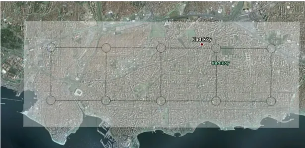
In order to evaluate the performance of the model and the efficiency of the proposed heuristic, we have generated some numerical applications. For this, some cities in Istanbul and a city in Ankara are chosen. We have deployed a grid topology to the selected areas since Robinson and Knightly (2007) have shown that grid topologies are more realistic in delivering the desired network performance.

First, we have located the grid topology with 1 mile distance between each MR. As we want to have high capacity on the links, we have placed them as close as possible as shown in the Figure 5.1.

(52)

38

Figure 5.1:Placed Grid Topology on Kadikoy

Then we have pointed the centers of each MR as shown in Figure.

Figure 5.2: Placed MRs on Kadikoy

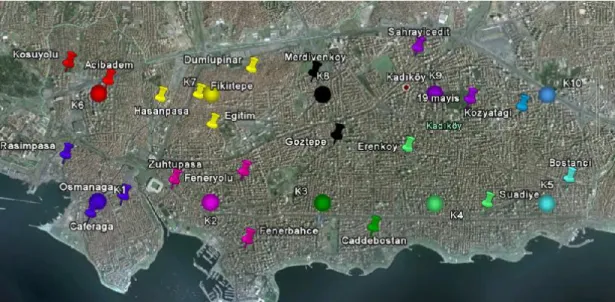
Finally, we have pointed the districts in the chosen cities and we have assigned each district to its nearest MR as shown in Figure. The same colors represent the assignment relations between each MR and the district.

(53)

39

Figure 5.3: Assigning Districts to the Placed MRs

We needed to remove some of the MRs from the system for two reasons: 1. If there is no district to be covered within the coverage range of the MR, 2. If the geographical conditions do not allow a MR deployment.

To use the advantages of mesh topology, we needed to make sure that each MR has at least 2 neighbors. For this reason, sometimes we needed to keep the MRs even if they are supposed to be removed from the system because of the conditions above.

The traffic demand of each MR is determined as follows: The total population assigned to the MR / 5000. In other words, we have assumed that 5000 people will need 1 mbps traffic load to be carried to the gateway node in each frame. Since the provided service level can be scaled, the number 5000 is not so important in this assumption.

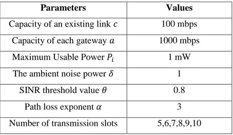
In order to have a grid topology, the ambient noise ratio and the SINR threshold value are chosen accordingly. The following table shows the parameters used in the examples.

(54)

40

Parameters Values

Capacity of an existing link 100 mbps Capacity of each gateway 1000 mbps

Maximum Usable Power 1 mW

The ambient noise power 1 SINR threshold value 0.8

Path loss exponent 3

Number of transmission slots 5,6,7,8,9,10

Table 5.1: The Parameters used in the Numerical Examples

The cities that are picked are: Kadikoy, Sariyer, Maltepe-Kartal, Pendik, Uskudar-Umraniye and Cankaya. For simplicity, we will use KAD, SAR, MAL, PEN, USK and CAN respectively. To define the number of gateways and the used transmission slots, we will use KAD_X_Y which corresponds exactly X gateways deployed and Y transmission slots are used in Kadikoy. The final networks of all areas can be seen in Appendix A, where each node represents a MR and the dashed lines represent the links between the MRs.

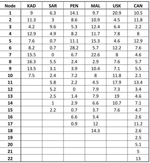
The table 5.2 shows the total traffic demand of each node deployed in the application areas.

The results in the Appendix are obtained by using GUROBI solver 4.5.0 on a 2.27 GHz, i5-M430 computer. We have limited the running time of each run with 3600 seconds.

(55)

41

Node KAD SAR PEN MAL USK CAN

1 9 6.3 14.1 9.7 20.9 10.5 2 11.3 3 8.6 10.9 4.5 11.8 3 4.2 9.6 5.3 12.4 6.4 2.2 4 12.9 4.9 8.2 11.7 7.8 8 5 7.6 0.7 11.1 15.3 4.6 12.9 6 8.2 0.7 28.2 5.7 12.2 7.6 7 15.5 0 6.7 22.6 8 4.6 8 16.3 5.5 2.4 2.9 7.6 5.7 9 13.5 3.1 3.9 10.4 7.1 5.5 10 7.5 2.4 7.2 8 11.8 2.1 11 5.8 2.2 4.5 17.9 13.4 12 5.2 0 7.9 7.3 3.4 13 2.5 1.4 7.9 19 4.6 14 1 2.9 6.6 10.7 7.1 15 2.2 0.7 3.7 7.6 4.7 16 6.6 3.4 2.6 17 0.9 12 11.2 18 14.3 2.6 19 2.5 20 5.1 21 5 22 13

Table 5.2: Traffic demands of each node deployed in the application areas

Let us consider the solution shown in the table below. For this table, we have used 5 transmission slots and up to 3 gateways are deployed to provide service. The first objective value is obtained by using one gateway in the area. This means if we deploy one gateway we can cover the 61.16% of the whole demand. In other words, rather than giving 5000 people 1 mbps in each frame, in the worst case we can give only 0.61 mbps. If we deploy 2 gateways in the area, then we can cover 132.45% of the demand which means they can transmit data much faster and they can increase their traffic demand up to 1.32 mbps.

(56)

42

m time (sec)

KAD_1_5 0.611621 1.86

KAD_2_5 1.3245 6.66

KAD_3_5 2.43902 1.78

Table 5.3: Solutions obtained for KAD

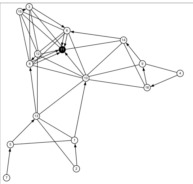
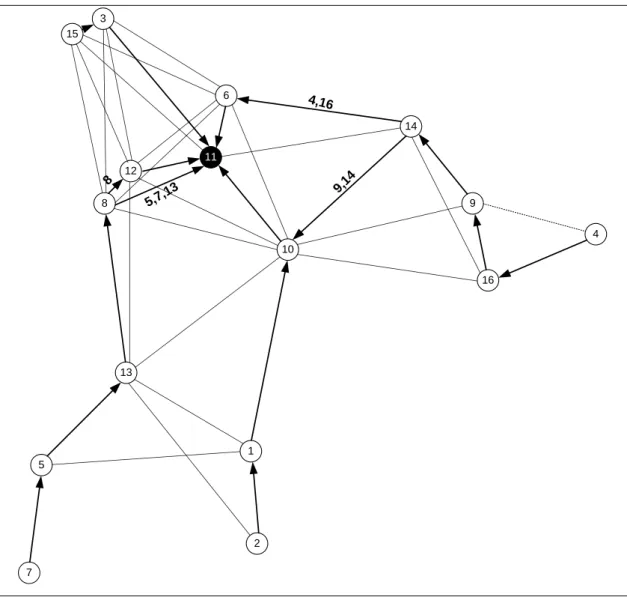
A solution found by is illustrated in Appendix F. In this solution, node 10 is picked as the gateway node and the traffic demand of each node is carried to that node in each transmission slot by activating non-interfering links.

(57)

43

Chapter 6

Extension

The routing structure of is commonly used in the literature and in the applications. However, we wanted to see the effect of a flexible routing rather than a tree-structured routing. Like the Multi Protocol Label Switching (MPLS) technology used in wired connections, each MR again has a single route to reach the gateway node but this time a node is allowed to send data to more than one node without dividing the traffic. Since each tree-structured routing is also feasible for the flexible routing, there is no surprise that the solution of the flexible routing will be at least as good as the solution of tree-routed structure.

In the remaining part of the chapter, we will formulate the model which uses flexible routing, define some valid inequalities for the model and compare it with the

(58)

44

6.1 Mixed Integer Linear Programming Model Using

Flexible-Routing

6.1.1 Variables

The following variables are needed to model the problem.

6.1.2 MILP Formulation Using Flexible-Routing

The following model is constructed for the problem defined earlier however rather than tree-routing, flexible-routing is used.

(59)

45

(60)

46

Our objective is again to maximize the fair service level provided to all customers while ensuring the constraints.

Constraint and are the upper bounds found earlier. Since the routing aspects have no impact on the calculation of these bounds, these upper bounds are still valid for .

is the capacity constraint which is same as the constraint used in WMN1.

Constraint means that if the traffic of node s is carried on the link, then that traffic can not be larger than the provided service level to all nodes times the traffic of node s. As one can easily see, constraint is non-linear. Following constraints, , and are used to linearize ;