RANGE-DOPPLER RADAR TARGET DETECTION USING DENOISING WITHIN THE
COMPRESSIVE SENSING FRAMEWORK
R. Akin Sevimli, Mohammad Tofighi, A. Enis Cetin
Department of Electrical and Electronics Engineering, Bilkent University, Ankara,Turkey
{sevimli, tofighi}@ee.bilkent.edu.tr, [email protected]
ABSTRACT
Compressive sensing (CS) idea enables the reconstruction of a sparse signal from a small set of measurements. CS ap-proach has applications in many practical areas. One of the areas is radar systems. In this article, the radar ambiguity function is denoised within the CS framework. A new de-noising method on the projection onto the epigraph set of the convex function is also developed for this purpose. This ap-proach is compared to the other CS reconstruction algorithms. Experimental results are presented1.
Index Terms— Compressive Sensing, Ambiguity Func-tion, Radar Signal Processing, Denoising.
1. INTRODUCTION
Compressive Sensing (CS) is a relatively recent approach used in various signal processing applications [1], [2], [3]. In [4], CS is applied to pulse compression, radar imaging and DoA estimation. One of the application areas is radar target detection using the ambiguity function [5]. Radar sig-nal processing is suitable for CS based denoising because of inherently sparse nature of signals in range-Doppler do-main [6], [7]. In many practical cases, the ambiguity function turns out to be very noisy. In this paper, the radar ambiguity function is denoised by using the CS framework. In Section 2, the CS framework is reviewed. In Section 3, the denoising solution is presented. In Section 4, simulation examples are presented.
2. COMPRESSIVE SENSING
CS framework is briefly reviewed below. Suppose that we have a one-dimensional vector v with length N . Any vector in N × 1 dimensions can be constructed using the a basis matrix, Ψ = [ψ1|ψ2|...|ψN]. The vector v can be formed as 1This work was supported in part by the Scientific and Technical Research Council of Turkey, TUBITAK. Any opinion, determination and conviction is not the official opinion of TUBITAK in the publication according to the contract. follows [8]: v = N X i=1 siψi or v = Ψs. (1)
If it is enough to represent the vector v with K << N ba-sis vectors, the signal is called K-sparse. In this case, mea-surements obtained by random projections can be sufficient to reconstruct the original signal.
y = Φv, (2)
where Φ is a M × N measurement matrix containing zero mean random numbers [2] and y represents the measure-ments. As a result, K-sparse vector y is expressed as follows: y = Θs = Φ.Ψ.s, (3) where Θ = Φ.Ψ is a matrix of size M × N . The vector v can be reconstructed using vector y provided that K < M < N . This problem can be solved as follows.
ˆs = min k s k1 such that y = Θs. (4)
Numerical algorithms were developed for this optimization problem. In addition, many other related optimization tech-niques are posed to solve this problem. It is shown that min-imizing the `1 norm forces small amplitude coefficients of s
vector to zero and it leads to a sparse solution. This paper uses the CS framework to denoise the Ambiguity Function (AF) used in range-Doppler radar target detection.
Transform domain noise reduction and filtering are widely used in practice. In this article, the AF is denoised using the measurement vector, y. During the reconstruction process, small amplitude AF values are forced to zero. As a result, denoising is achieved. This leads to better target detection results in radar signal processing.
3. AMBIGUITY FUNCTION AND RANGE-DOPPLER TARGET DETECTION
Ambiguity function (AF) is generally used to determine sim-ilarities between two signals [9]. In radar signal processing,
ambiguity function is a two-dimensional equation defined in range-Doppler plane [10]. The position and velocity of targets in the environment can be determined from this equation. The AF is defined as follows:
ξ[l, p] =
N −1
X
i=0
ssurv[i]s∗sref[i − l]e −j2πip
N , (5)
where ssurv[i] and ssref[i − l] represent surveillance and
ref-erence signals, respectively. The index l is the range axis and p represents the Doppler axis. Let bl[i] = ssurv[i]s∗sref[i − l].
When bl[i] is inserted to AF, we obtain the following
equa-tion: ξ[l, p] = N −1 X i=0 bl[i]e− j2πip N , (6) f or l = 0, 1, ..., L, p = 0, 1, ..., N − 1.
Ambiguity Function can be calculated by computing the FT of bl[i] using the FFT algorithm. Targets form peaks in 3-D
range-Doppler map as shown in Fig. 1. In Figures 2 and 3, Doppler frequencies and bistatic ranges of 6 targets are shown. In this example, the sampling frequency, fsand
in-tegration time are 2 × 10⁵ Hz and 1 sec., respectively. As a result, the length of surveillance and reference signal is 2 × 10⁵. This discrete-time signal s decimated in time and
the length of signals is reduced to N = 4096. After this point, Doppler frequency axis is focused between −500 and 500 Hz to show targets clearly. In Figures 1-3, the L = 150 and p = −500, ..., 500 are shown.
The AF is a sparse function of l and p. For instance, there are 6 targets with different velocities in Fig. 1. There is no other important values other than these 6 range-Doppler target locations. Because of this reason, AF has an ideal structure for compressive sensing based denoising. Suppose that our
Fig. 1: 3-D range-Doppler frequency graph obtained using AF computed using FFT as in Equation 5.
measurement matrix, Θ is an M × N matrix. In this case, the compressed measurements can be calculated for each row of
Fig. 2: Doppler frequency graph obtained using AF computed using FFT as in Equation 5.
Fig. 3: Bistatic range graph obtained using AF computed us-ing FFT as in Equation 5.
the AF as follows:
yl= Θ.ξl, (7) f or l = 0, 1, ..., L.
where the vector, ξl is the l-th row of ξ(l, p) and its size is
N = 4096, which is also the size of FFT in (5) and (6); the vector ylis of size M , which is much smaller than N because the measurement matrix Θ is an M × N . In this article, M is approximately selected as M = 400 ∼= 0.1 × N and the CS problem is posed as reconstruction of ξ[l, p] from ylvectors. Since sparsity assumption is used, denoising is also achieved during the CS reconstruction.
In this paper, various optimization algorithms are used for denoising. These are Basis Pursuit (BP) [11], Orthog-onal Matching Pursuit (OMP) [12], Compressive Sampling Matched Pursuit (CoSAMP) [13], and Projections onto Epi-graph Set of a Convex cost function (PES-`1) based
denois-ing [14].
3.1. Basis Pursuit (BP)
Basis Pursuit (BP) tries to find signal representations with convex optimization. Each measurement vector, yl is used in the following minimization problem:
min k yl− Θξlk22+λ k ξlk1, (8)
where λ is the regularization parameter determining the spar-sity level of the solution. The above CS reconstruction
prob-lem is solved for each row of the AF function l = 0, 1, ..., L = 150.
3.2. Orthogonal Matching Pursuit (OMP)
Orthogonal Matching Pursuit (OMP) is a greedy algorithm that also determines a sparse solution to the CS problem. It is an extension of the Matching Pursuit (MP) algorithm. Ad-vantages of this algorithm are its speed and computational efficiency. It is also used at the output of the matched filter to find the strongest target [15]. To reconstruct the vector ξl,
this algorithm first tries to find which columns of Θ contribut-ing most to the observation vector yl. During each iteration,
columns of Θ are picked and correlated with the remaining parts of yl. Contribution of yl is subtracted and iterated on
the residual. After M iterations, this algorithm finds a set of columns from the basis set representing the vector ξl. 3.3. Compressive Sampling Matched Pursuit (CoSAMP) Compressive Sampling Matched Pursuit (CoSAMP) is an it-erative greedy algorithm that recovers a compressible signal from its noisy samples. It is efficient for same problems. It requires a measurement vector Θ, observation matrix yl, a
sample of noisy vectors ξland a stopping criterion. The
fol-lowing Algorithm 1 is implemented to solve the CS problem: Algorithm 1 CoSAMP
1: Inputs:
Θ, yl, ξl, k, stopping criterion 2: Initialize:
r = yl, ξ0l = 0, k = 0, Γ = ∅ 3: While: not converged
4: Proxy: bv = Θ∗r 5: Identify: Ω = SD(bv, 2k) 6: Merge: T = Ω ∪ Γ 7: Update: bξl= argminξ k yl− Θξlk 8: Γ = Ω = SD( bξl, 2k) 9: ξk+1l = PΓξbl 10: r = yl− Θξ k+1 l 11: k = k + 1 12: End while: 13: Output: bξl= ξkl
3.4. Projections Onto Epigraph Set Of A Convex Cost Function (PES-`1)
Projections Onto Epigraph Set Of A Convex Cost Function (PES-`1) is a new signal processing framework described in
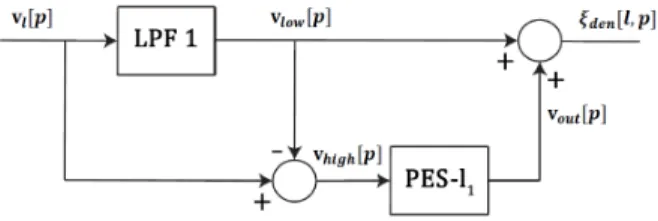
[16, 17]. In this new denoising method, each row of the mag-nitude of AF data: vl[p] = |ξ[l, p]| is first filtered by a
high-pass filter with cut-off π/4 (normalized angular frequency) and subtracted from the original data producing a low-pass
filtered version vlow[p]. Let the high-pass filtered version
be vhigh[p]. The signal vhigh[p] is projected onto the
epi-graph set of `1-norm function. The output of the
projec-tion operaprojec-tion vout[p] is combined with the low-pass signal
|vlow[l, p]| to obtain the denoised version of |ξ[l, p]| as
dis-cussed in [18–20]. This denoising method takes advantage of the sparse nature of data and it does not require any measure-ment matrix. The block diagram of the denoising structure is shown in Figure 4.
Fig. 4: The block diagram of PES-`1algorithm.
4. EXPERIMENTAL RESULTS
In this section, simulation examples using BP, OMP, CoSAMP, and PES-`1 are presented and they are compared to each
other. Reference and surveillance stereo FM signals are cre-ated for passive radar scenario and it contains 6 targets as summarized in Table 1. In radar signal processing, surveil-lance and reference signals are first passed through an LMS adaptive filter to suppress the clutters. Range-Doppler map is obtained after LMS filtering in all cases. The M × N
mea-Table 1: System Scenario
Target 1 Target 2 Target 2 Target 2 Target 2 Target 6
Bistatic Range(Km) 20,25 60 60 99,75 110,25 129,75
Doppler Frequency(Hz) 150 -250 50 300 -150 -300
SNR(dB) 4,1 -3,8 -20,8 -21,1 -21,6 -22,1
surement matrix Θ is constructed from randomly weighted Fourier coefficients in all cases as discussed in [2]. In all the examples, the N = 4096 and M = 400, respectively.
size. For all the reconstruction methods, randomly weighted Fourier coefficients are used because the mea-surement matrix contains random numbers. In general, signal length and length of the compressed data are N = 4096 and M = 400, respectively. This means that a vector of size 4096 is represented by 400 and this vector is sufficient to represent each row of each AF data.
In Figure 5 (6, 7 and 8), the range-Doppler map for BP (OMP, CoSAMP and PES-`1) methods are shown,
respec-tively. Generally, targets with higher SNR at 150 and −250 Hz are clearly detected for all of cases, but low SNR targets are not visible in Figure 5, 6 and 7. PES-`1algorithm is the
only method that can detect all targets shown in Figure 8. In Figure 9, the receiver operating characteristics (ROC) curves
Fig. 5: Range-Doppler map for BP algorithm.
Fig. 6: Range-Doppler map for OMP algorithm.
Fig. 7: Range-Doppler map for CoSAMP algorithm. for all the methods are shown. The ROC curve is plotted by using the Constant False Alarm Rate (CFAR) algorithm with different thresholds. The parameters of the CFAR algorithm are training cell size=10, guard cell size=10 and the probabil-ity false alarm Pfa=0.1. As can be seen from Figure 9, PES-`1outperforms other reconstruction algorithms. In Figure 9,
FFT based method computed using Equation 5 and 6 denotes the observed noisy data shown in Figure 1. In addition, an-other set of measures used in denoising is the PSNR and SNR. PSNR and SNR values are calculated by using range-Doppler map and presented in Table 2. As shown in Table 2, PES-`1
has higher PSNR and SNR values with 48, 71 dB and 9, 16
Fig. 8: Range-Doppler map for PES-`1algorithm.
Table 2: PSNR and SNR values of reconstruction methods.
PSNR (dB)
SNR (dB)
CoSAMP
48,65
8,93
PES-`
148,71
9,16
OMP
42,27
-2,37
BP
44,83
0,96
FFT
43,54
-0,79
dB, respectively. Some algorithms, such as OM P have even less PSNR and SNR values than FFT method.
Fig. 9: Receiver operating characteristics (ROC) curve with different thresholds.
5. CONCLUSION
In this paper, radar ambiguity function used in a passive bistatic radar scenario is denoised using various CS recon-struction algorithms (BP, OMP, CoSAMP and PES-`1). It is
experimentally observed that CS based denoising removes noise and helps the detection of process of targets. The most successful denoising results are obtained using the PES-`1
REFERENCES
[1] Christian R Berger, Zhaohui Wang, Jianzhong Huang, and Shengli Zhou, “Application of compressive sensing to sparse channel estimation,” Communications Maga-zine, IEEE, vol. 48, no. 11, pp. 164–174, 2010. [2] David L Donoho, “Compressed sensing,” Information
Theory, IEEE Transactions on, vol. 52, no. 4, pp. 1289– 1306, 2006.
[3] Michael Lustig, David Donoho, and John M Pauly, “Sparse mri: The application of compressed sensing for rapid mr imaging,” Magnetic resonance in medicine, vol. 58, no. 6, pp. 1182–1195, 2007.
[4] Joachim HG Ender, “On compressive sensing applied to radar,” Signal Processing, vol. 90, no. 5, pp. 1402– 1414, 2010.
[5] Oguzhan Teke, Ali Cafer Gurbuz, and Orhan Arikan, “A robust compressive sensing based technique for re-construction of sparse radar scenes,” Digital Signal Processing, 2013.
[6] Matthew Herman and Thomas Strohmer, “Compressed sensing radar,” in Radar Conference, 2008. RADAR’08. IEEE. IEEE, 2008, pp. 1–6.
[7] Richard Baraniuk and Philippe Steeghs, “Compres-sive radar imaging,” in Radar Conference, 2007 IEEE. IEEE, 2007, pp. 128–133.
[8] Richard G Baraniuk, “Compressive sensing [lecture notes],” Signal Processing Magazine, IEEE, vol. 24, no. 4, pp. 118–121, 2007.
[9] T Tsao, M Slamani, P Varshney, D Weiner, H Schwarz-lander, and S Borek, “Ambiguity function for a bistatic radar,” IEEE Transactions on Aerospace and Electronic Systems, vol. 33, no. 3, pp. 1041–1051, 1997.
[10] F Colone, DW O’hagan, P Lombardo, and CJ Baker, “A multistage processing algorithm for disturbance re-moval and target detection in passive bistatic radar,” IEEE Transactions on, Aerospace and Electronic Sys-tems, vol. 45, no. 2, pp. 698–722, 2009.
[11] Shaobing Chen and David Donoho, “Basis pursuit,” in Signals, Systems and Computers, 1994. 1994 Confer-ence Record of the Twenty-Eighth Asilomar ConferConfer-ence on. IEEE, 1994, vol. 1, pp. 41–44.
[12] Joel A Tropp and Anna C Gilbert, “Signal recovery from random measurements via orthogonal matching pursuit,” IEEE Transactions on Information Theory, vol. 53, no. 12, pp. 4655–4666, 2007.
[13] Deanna Needell and Joel A Tropp, “Cosamp: Iterative signal recovery from incomplete and inaccurate sam-ples,” Applied and Computational Harmonic Analysis, vol. 26, no. 3, pp. 301–321, 2009.
[14] M. Tofighi, K. Kose, and A. Enis Cetin, “Signal
re-construction framework based On projections onto epi-graph set of a convex cost function (PESC),” ArXiv e-prints 1402.2088, Feb. 2014.
[15] Christian R Berger, Bruno Demissie, J¨org Heckenbach, Peter Willett, and Shengli Zhou, “Signal processing for passive radar using ofdm waveforms,” Selected Topics in Signal Processing, IEEE Journal of, vol. 4, no. 1, pp. 226–238, 2010.
[16] A. E. Cetin, A. Bozkurt, O. Gunay, Y. H. Habiboglu, K. Kose, I. Onaran, R. A. Sevimli, and M. Tofighi, “Pro-jections onto convex sets (pocs) based optimization by lifting,” IEEE GlobalSIP 2013, Austin, Texas, USA, Dec 2013.
[17] Giovanni Chierchia, Nelly Pustelnik, Jean-Christophe Pesquet, and B´eatrice Pesquet-Popescu, “Epigraphical projection and proximal tools for solving constrained convex optimization problems: Part i,” CoRR, vol. abs/1210.5844, 2012.
[18] A. Enis Cetin and Mohammad Tofighi, “Denosing us-ing wavelets and projections onto the l1-ball,” ArXiv e-prints 1406.2528, Jun 2014.
[19] M. Tofighi, K. Kose, and A.E. Cetin, “Denoising using projections onto the epigraph set of a convex cost func-tion,” IEEE 21st International Conference on Image Processing (ICIP2014), Oct 2014.
[20] Kivanc Kose, Volkan Cevher, and A Enis Cetin, “Fil-tered variation method for denoising and sparse signal processing,” in Acoustics, Speech and Signal Process-ing (ICASSP), 2012 IEEE International Conference on. IEEE, 2012, pp. 3329–3332.