Josephson effect in hybrid superconductor-normal metal structures

J O S E P K S O N ^ E F F E C T m

SUPERCONDUCTOR N O R M A L METAL

.

DEPARTMENT' OF PHYSICS' :.

'S b 'T H E iN

OF.ENGlNEERiNG AND SOENCE

IN PARTIAL FULFILLMENT OF THE REQUIREMENTS

FOR THE DEGREE OF

■

MASTER OF SCIENCE' '

o c

6/ Z

^ S 8

CSS

«

2 .0 0 0

S e i3 te 5 iib e r

2000

JOSEPHSON EFFECT IN HYBRID

SU PER C O N D U CTO R -N O R M AL METAL

STRUCTURES

A THESIS

SUBMITTED TO THE DEPARTMENT OF PHYSICS AND THE INSTITUTE OF ENGINEERING AND SCIENCE

OF BILKENT UNIVERSITY

IN PARTIAL FULFILLMENT OF THE REQUIREMENTS FOR THE DEGREE OF

MASTER OF SCIENCE

By

Özgür Çakır

September 2000

η

cfi

a

о

d

· сО

о

Ό о < rí ίS ^t>

L'X

-e r

I certify that I have read this thesis and that in my opinion it is fully adequate, in scope and in quality, as a dissertation for the degree o f Master o f Science.

Prof. Igor Kulik (Supervisor)

I certify that I have read this thesis and that in my opinion it is fully adequate, in scope and in quality, as a dissertation for the degree o f Master o f Science.

7 \ r : / A ^ t. Proh ^afer Gedik

I certify that I have read this thesis and that in my opinion it is fully adequate, in scope and in quality, as a dissertation for the degree o f Master o f Science.

Asst. Prof. Alexander Goncharov

Approved for the Institute o f Engineering and Science:

Prof. M ehm ^Baray,

Abstract

JO SE P H SO N EFFECT IN H Y B R ID

S U P E R C O N D U C T O R -N O R M A L M ETAL

STR U C TU R ES

Özgür Çakır

M. S. in Physics

Supervisor: Prof. Igor Kulik

September 2000

The clean SNS junction, with a phase difference

x

across the normal metal barrier and without Fermi level mismatch between the components, is modeled by a step like pair potential. The quasiclassical equations are obtained from the Gorkov equations by the elimination of crystal momenta and are valid in the existence o f only the off-diagonal potential(pair potential). Then for the

SNS

junction, the quasiclassical Green functions are obtained. At zero temperature, in the long barrier lim it(d ^ ^o)> the current is found to have a sawtooth dependence on the phase difference, the amplitude of which is inversely proportional to the thickness of the normal layer. At finite temperatures in the limits

d

and

Tc

T,

the current is found to have exponential dependence on the thickness of the normal layer,

T

ex p (—d/^

7

’) sin y , .where = vf

I2

tt

T.

An extension o f single

SNS

structures is the periodic

SNS

structure which may as well exhibit Josephson effect. It is simulated by a periodic step-wise pair potential, where the phase o f the pair potential changes by some constant value in subsequent superconducting islands. Bogoliubov equations in the semicla.ssical

limit are employed, yielding the density of states(DOS). In the DOS, there appears some forbidden energy regions, which point out to a band structure.

K e y w o r d s : Superconductivity, Josephson Effect, Hybrid Structures, Weak Links, Proximity Effect, Quasiclassical Green Functions, Bogoliubov-de Gennes Equations

özet

Özgür Çakır

Fizik Yüksek Lisans

Tez Yöneticisi: Prof. Igor Kulik

11 Eylül 2000

Ustüniletken elektrotlar arasında

x

kadar faz farkı olan ve bileşenleri arasında Fermi seviyesi farkı bulunmayan saf

SN S

eklemi, basamak şeklinde bir çift potan­ siyel modeli ile incelenecektir. Ancak çapraz olmayan potansiyellerin varlığında geçerli yan-klasik denklemler, Gorkov denklemlerinden örgü momentumunun elimine edilmesiyle elde edilmekte ve

SNS

eklemi için çözülmektedir. Sıfır sıcaklıkta, kalın bariyer limitinde Josephson akımının faz farkına bağlılığının doğrusal olduğu ve büyüklüğünün normal tabaka kalınlığıyla ters orantılı değiştiği gösterildi. Düşük sıcaklıklarda,

d

Tc

T

limitlerinde akımın

T

exp( —d / s i n

x

şeklinde, normal tabakanın kalınlığına üstel şekilde bir bağlılık gösterdiği bulunmuştur(^

7

’ = vf

/2

tt

T).

Peryodik

SNS

yapısı bcisamak şeklinde periyodik çift potansiyel modeli ile ele alınacak ve üstüniletken adacıkların fazları her periyotta aynı miktarda artmaktadır. Bu sistem için Bogoliubov-de Gennes denklemleri yan-klasik limitte çözülmekte ve durum yoğunluğu elde edilmektedir. Enerji spektrumunda yasak enerji bölgelerinin varlığı bant yapısına işaret etmektedir.

Anahtar

s ö z c ü k le r : Josephson etkisi, zayıf bağlantılar, melez yapılar, Bogoliubov-de Gennes Bogoliubov-deklemleri, yan-klasik Green fonksiyonları

Acknowledgement

I would like to thank to Prof. Igor Kulik for his guidance during this research. I would also like to thank to M. Ali Can, Isa Kiyat, Selim Tanriseven, Feridun Ay, Kerim Savran, Emre Tepedelenlioglu, Başak Kaptan, İlke Yılmaz who kept my motivation high all the time.

I am indebted to my family for their continuous support and care. Last but not the least I’m grateful to Elif.

Contents

Abstract iii

Özet V

Acknowledgement v

Contents vi

List of Figures viii

List of Tables ix

1 Introduction 1

2 Bogoliubov-de Gennes and Gorkov Equations 10

2.1

Bogoliubov-de Gennes E q u a t io n s ... 10

2

.

1.1

Self Consistency C on d ition ... 14 2.1.2 Continuity Equation and the Current Expression for

Bogoliubov-de Gennes E q u a t io n s ... 16 2.1.3 Excitation Spectrum of a Superconductor ... 17 2.2 Andreev R e fle c t io n ... 18 2.3 Tight Binding Approach and Lattice Bogoliubov-de Gennes

E q u a tio n s ... 21 2.4 Green Functions and Gorkov E qu ation s...

22

3 Josephson Effect in Single SNS Structure 25

3.1 Gorkov Equations in One D im e n s io n ... 25

3.1.1 Green Functions for the Bulk Superconductor and Metal . 27 3.2 Introduction of Quasiclassical Green F u n ction s... 29

3.2.1 Application of the Quasiclassical Equations to the Bulk Superconductor with Constant P h a s e ... 32

3.3 Calculation of the Josephson Current Through a Single SNS stru ctu re... 35

4 Band Structure of Periodic SNS Structures 43 4.1 One Dimensional BdG E q u a tio n s ... 45

4.2 Semiclassical A pp roxim ation ... 46

48 4.3.1 Andreev R e fle c tio n ... 50

4.3.2 Discrete Spectrum of the Single SNS S tru ctu re... 51

4.4 Symmetries o f the Bogoliubov-de Gennes Equations for the Periodic SNS S tru ctu re...

53

4.5 Solution of the Semiclassical Equations for the Periodic SNS stru ctu re... 55

4.6 DOS for the ID Periodic SNS S tructure... 57

4.7 DOS for the Three Dimensional C a s e ... 61

4.8 Josephson Current Through the Periodic SNS S tru ctu re... 62

5 Conclusion 64

List of Figures

1.1

Behavior of phase near a tunnel barrier located at x

= 0

...

2

1.2

(a)SIS (b)SNS (c)ScS type Josephson junctions ...

3

2.1

Schematic of Andreev reflection:Electron reflects back as a hole,

then the hole reflects back as an electron at the

S

boundary, meanwhile they pick up a phase at the interfaces...

20

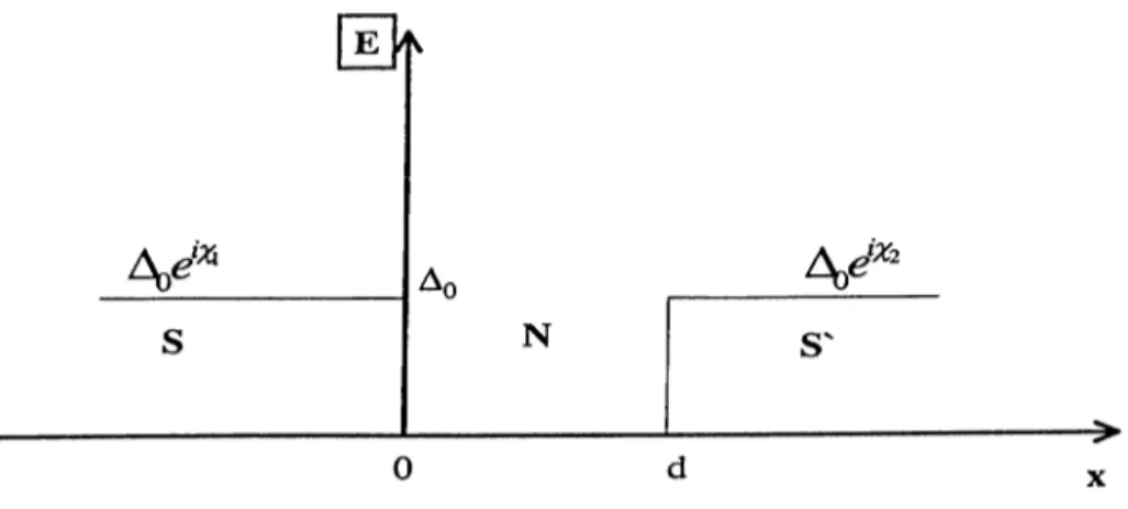
3.1 Single SNS structure with phase difference

x

across the barrier . .

35

3.2 Phase dependence of Josephson current at T = 0 ... 42 4.1 Periodic structure where the phase of the gap parameter is

changing in a cyclic manner...

43

4.2

Andreev Reflection: An electron incident on a superconducting

wall reflects back as a hole, meanwhile picking up a phase with a slight momentum nonconservation of —

2

A „ ... 48 4.3 Discrete spectrum of quasi-particles in a normal metal confined by

superconducting banks... 51 4.4 DOS for values of

(p

between

0

and 27T for

a = +

where

a

=

2^o,l> =

2^0-

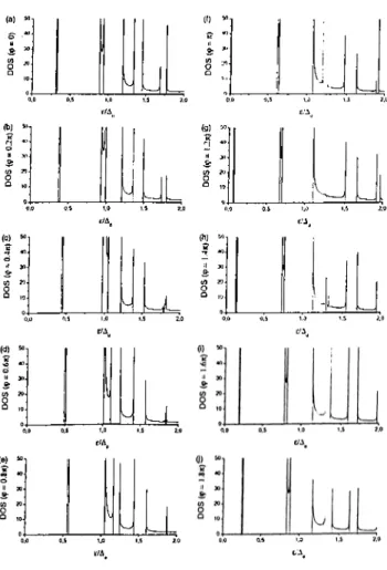
Energy is scaled with respect to Aq, and DOS is scaled with

respect to number of unit cells in the specimen... 59

4.5

DOS for values of

<p

between

0

and

2ir for cr = +

where

a =

=

4

(^

0

· Energy is scaled with respect to Ao, and DOS is scaled with respect to number of unit cells in the specimen... 60

Chapter 1

Introduction

In 1962 Josephson predicted the existence o f a super-current between two superconducting electrodes separated by a tunnel barrier (thin insulating layer), ^

Is = Ic

sin Ay? (1.1)

without any voltage drop across the barrier, which is called the

stationary

Josephson effect. Ic

is the maximum value o f the supercurrent that the barrier can support, which is, at the same time, a measure o f coupling between two electrodes. Ay?

= (pi —

is the phase difference o f the order parameters o f the electrodes across the interface.

^

1,2

= (1.2)

where ■0 is the Cooper pair amplitude. In the presence of a constant voltage difference

V

across the barrier, the supercurrent oscillates in time.

dAp _ 2eV

and is called the

nonstatinary Josephson

effect.

Josephson effect is a remarkable manifestation of macroscopic coherence of the superconducting state. Macroscopic coherence is maintained by the existence of a macroscopic order parameter

ip =

characterizing the Cooper-pairs(paired electrons) inside the whole specimen,

\ipŸ

being the local value of the Cooper-pair density,

ip

varies at distances of the order of coherence length which is much larger than atomic length scales.

Tc

is the critical temperature of the superconductor. The macroscopic coherence, first postulated by London,^ was phenomenologically formulated by Ginzburg and Landau in 1950 and they have showed that the order parameter

ip

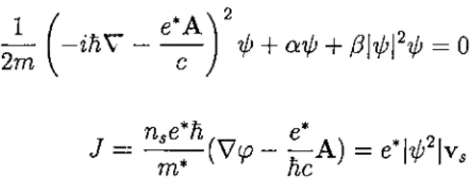
obeys a Schrodinger like equation,^ with a corresponding conserved current.

CHAPTER 1. INTRODUCTION 2

2m

ih V

-e*A'

Ip + aip

-f

^\ipf‘ip =

0

(1.4)

n,e'h

e’

2

^ I''*

ng = \ip\'^

is the local value o f the density of Cooper pairs, Vs is the local superfluid velocity and A is the vector potential, e*,

m*

are the charge and mass of the Cooper pair respectively.

T h ia insulating layer

CHAPTER 1. INTRODUCTION

The existence of macroscopic phase coherence manifests itself in a number o f macroscopic quantum effects like (i)Josephson e ffe ct/ (ii)quantization of magnetic flux in a supercon du ctor/(iii) periodic variations o f depression in the transition temperature o f a hollow superconducting cylinder, with varying magnetic flux(Little-Parks Effect).^

Supercurrent through a tunnel junction is accompanied by a jum p in the ifliase at the barrier and is a function of the phase difference

(pi — (p

2 between the two sides of the interface, which is expected due to gradient term in the current expression (

1

.

5

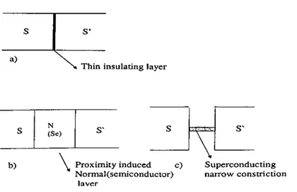
)(F ig -l.l).

The tunnel junctions (SIS) were treated by tunneling Hamiltonian approach, on the grounds that i)the thickness of the barrier is much smaller than any other characteristic length(particularly f, mean free path o f the electron and coherence length respectively) so that the processes inside the barrier can be ignored ii)the transparency of the barrier should be so small that the critical current that the barrier can support is much less than the critical current of the electrodes, so that perturbation with respect to transparency o f the barrier can be a p p lied /’®’^’®’®

b)

s S’

a)

% Thin insulating layer

S N(Se) S ' S

\

S'

Proximity induced c) Superconducting Normal (semiconductor) narrow constriction

laver

CHAPTER 1. INTRODUCTION

However Josephson junctions are not limited by tunnel junctions. Apart from tunnel barrier, Josephson effect can take place in a conducting junction between superconducting electrodes, the critical current through which is much smaller than that o f the superconducting e le ctro d e s.T h e se junctions are the so called w ea k links which may be achieved using a superconducting connection o f small cross-section, or using a substance which is not superconducting, which may be a normal metal or a semiconductor(Fig.l.

2

). Finite conductivity of the weak link is the main distinguishing property and processes going on inside the junction are taken into account.

Even if the link is normal or semiconducting, it exhibits weak superconducting property due to proximity effect which arises due to leakage of Cooper pairs from the superconducting electrodes into the normal or semiconducting region. The weak links are more advantageous over tunnel junctions, o f being low capacitance, of experimental reproducibility, enabling analysis of reduced space dimensionality. Recently there’s a growing interest in construction o f novel devices using weak links.

Previously, especially during 1970’s, although the transport properties of superconducting-normal, semiconductor hybrid structures were extensively studied, because of complications in growing hybrid nano-structures, there hasn’t been been any experimental success till 1991.^®’^°

Inl958 Bardeen, Cooper and Schrieffer founded the microscopic theory of su p ercon d u ctivity .T h e ground state of the superconductor is the state in which the electrons with energy in the |A| neighborhood of the Fermi energy, i.e. in the interval

{E —

|A|, E -I- |A|) are all condensed into Cooper pairs. A is an off- diagonal potential(also called the pair potential) which is proportional to Cooper pair amplitude "0. At finite temperatures, electron-type and hole-type quasi­ particles are excited. The two component wave function with the components ■

06

)

Oh,

which are electron and hole-type excitations respectively, is governed by Bogoliubov-de Gennes equations(BdC),^°’^^ with A serving as the off-diagonal potential.

CHAPTER 1. INTRODUCTION

(He

+ C/)^e(r) + A(r)(/)/j(r) =

eOeir)

A*(r)^e(r)

-

{He

+

U)(f>h{r)

=

ephir) (1.5)

U

and A are the self consistent potentials,

u(r) = -v'E(№.»WlV« + l'Ata(r)|’(i-/„))

n

M r)

=

V £ ( ^ U r ) " M r ) ( l - 2/.))

(1.6)

U

is the usual Hartree-Fock term, and A is the pair potential. Since the BdG equations enable a spatial analysis, it is a powerful tool in handling normal-

uperconductor interfaces.

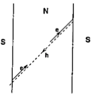
In 1965, Andreev discovered a new scattering mechanism which realizes in case of a sharp spatial variation of the off-diagonal potential A.^^ In normal region an electron (hole) of energy lower than the gap(|A|), incident at the superconducting interface reflects back as a hole(electron), accompanied by the creation (annihilation) of a Cooper pair in the superconducting region. Consequently, in a normal metal confined by superconducting specimen, for energies such that

E <

|A|, the energy spectrum becomes discrete as was predicted by Kulik.^^ When the energy o f the excitation is larger than the gap parameter, partial Andreev reflection occurs. Andreev reflection is the only scattering mechanism in the mere existence o f an off-diagonal potential.

Creen’s function method is a powerful tool in the study o f superconductivity.^® Single particle temperature Creen’s functions provide full information about the excitation spectrum and the density of states o f quasi-particles. Single particle temperature Creen’s function is defined as follows

CHAPTER 1. INTRODUCTION

where indicates time ordered product and < ... > is the thermodynamic Gibbs average, are the fermion field operators. On the other hand Gorkov Green’s function is defined as

F*{rr,T'r') = - <

T ,i'|(rr)'I't(rV ) >

(1.8)

One particle Green’s function and Gorkov Green’s function in the imaginary frequency domain, satisfy the Gorkov equations,

^

O +

r') = i(r - r')

+ ^ + /z) FJ(r, r') - A*(r)

G^{t,

r') = 0

(1.9)

with the self consistency condition,

A(r) = FF^(rr+,rr).

(1.10)

V

is the electron-phonon coupling constant. In its present form, Gorkov equations are only applicable to equilibrium situations.

Since the Gorkov’s equations are space dependent, they can be employed in studying superconductor-normal hybrid structures.

Zero voltage current through a surface

S

separating two regions o f space, is expressible in terms of one particle Green’s functions.

j = 2 ie T {f

[

JreV' Jr'eV

- i f

)d“rdV T^A (r)A ‘ (r')GS(r-r')G-„(r',r)

(Ul)

J reV J r'eV '

which is a quite general, powerful formula derived by Josephson^·^ and Kulik^® independently.

Gu{x — x')

is the full Green’s function and

G^{x — x')

is that of the bulk normal metal.

V

and

V

are the volumes on the opposite sides of surface

S.

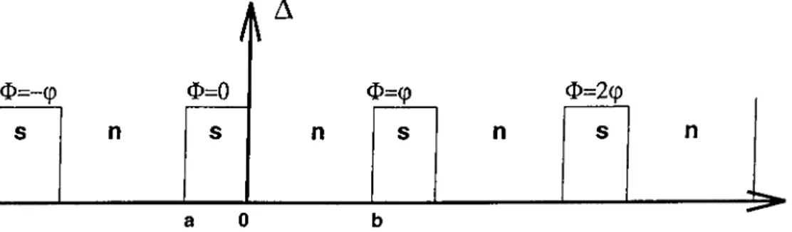
This current expression can be employed in order to calculate the zero voltage Josephson current, as long as the Green’s functions are known for the particular system.

In the third chapter we will study Josephson effect in

SNS

structure (Fig.3.1) with vanishing pair potential in

N

region, and pair potential A

1,2

= Aoe*^‘ ·* in

S, S'

banks respectively. The excitation spectrum and density o f states, as well as the Green’s functions depend on the phase difference between the superconducting banks.

The dc Josephson current in a clean

SNS

structure was first studied by Kulik^^’ ^® After determining the quasiparticle wave functions, he constructed Green’s functions in terms of the quasi-particle wave functions. Following Kulik, Ishii^^ found the exact Green’s functions, first expressing the Green’s functions in the form of bulk Green’s function plus the bilinear products o f bulk Green’s functions with the corresponding coefficients. Then he determined the coefficients using the integral equations generated by the Gorkov’s equations. After determining the Green’s functions both Kulik and Ishii employed the current expression(

1

.

11

) in order to determine the Josephson current. On the other hand, Bardeen and Johnson employed the Landau’s Galileian transformation principle for excitations in a superfluid in order to obtain the current.

Since the current through

SNS^

in steady state does not dissipate, the system is in a thermodynamical state. Thus the phase difference of coupled superconductors can be taken as a thermodynamical variable.^'^’^®’^^ Once the phase dependent density of states is known, the thermodynamic potential can be written as

CHAPTER 1. INTRODUCTION 7

1

r°°

Josephson current is nothing but the response of thermodynamic potential to the phase difference x, CHAPTER 1. INTRODUCTION 8

J{x)

= -

2

e

dx

1 roo

= 2 e -

dEln(l + e-^^)

¡J Jo

_Ox

(1.13) (1.14)

Due to proximity effect, there is a leakage of Cooper pair condensate from the superconductor to the normal region which makes the normal metal exhibit superconducting properties. In the existence o f a phase difference between the superconducting banks, there appears an effective gap in the normal region, which giv^es an explaination o f the superconducting property exhibited by the normal region in

SNS.

Since superconductivity is a macroscopic phenomenon, the coherence length(^o = vf

/A

xq

)

relevant to superconductivity is much larger than the atomic scales, which gives the idea o f filtering out the crystal momentum, being left with the mere information of superconductivity. However elimination of crystal momentum is only possible when the crystal momentum is conserved, i.e., it is required that only the off-diagonal potential A exists.

The quasi-classical Green’s functions will be found by the elimination of crystal momenta from the Gorkov’s equations thus obtaining the equations and the boundary conditions satisfied by them. The differential equations satisfied by quasiclassical are o f first order and the boundary conditions are easy to handle. The quasi-classical Green’s functions can only be applied when there is only off-diagonal potential A , i.e., when there’s no diagonal scattering. Then the quasiclassical equations are going to be solved for single

SNS

structure obtaining the quasi-classical Green’s functions for this structure. Then making use o f (1.11) the supercurrent will be obtained at T =

0

and at finite temperatures.

In the fourth chapter we will be studying periodic

SNS

structure with cyclic variations o f the phase o f pair potentials in

S

islands. (Fig.4.1) In other words, the

CHAPTER 1. INTRODUCTION

phase is increasing in each period by some constant value, where the modulus of the pair potential remains unchanged. For this structure the spectrum and density of states o f quasi-particles will be studied.

SNS

periodic structure with all superconducting islands of the same phase, was first studied by Van Gelder in 1 9 6 8 . The interesting feature about the periodic

SNS

structure with cyclic phase is the possibility o f a Josepson effect. First of all, Bogoliubov-de Gennes equations will be linearized by employing semi-classical approximation,^^ the idea of which is nothing but elimination o f crystal momenta from the Bogoliubov-de Gennes equations. Semiclassical equations are valid as long as the crystal momentum is conserved. The semi-classical equations are solved for the

SNS

periodic structure with cyclic phase thus obtaining the density of states which enables one to write an expression for the Josephson current through this structure.

Chapter 2

Bogoliubov-de Gennes and

Gorkov Equations

2.1

Bogoliubov-de Gennes Equations

Electrons with an attractive potential can be described by a method which is a generalization of Hartree-Fock method, in order to describe superconductiv­ ity (Bogo/iu bo v,i 959).^° The quasi electron and hole excitations can be shown to obey an equation similar to Dirac equation. The Hamiltonian describing the electrons consists of Hamiltonian with an external potential and the two body attractive delta-Dirac potential between electrons. The electronic Hamiltonian without interactions is

He = I dh

a=n

(P -

eAŸ

2m

+ U„(r)

’F (ra ) —

Ep

(2.1)

where

U

q is an external potential which is taken to be spin indepen­ dent (considering nonmagnetic materials), and

Ep

is the Fermi energy. The field operators satisfy the anticommutation relations

CHAPTER 2. BOGOLIUBOV-DE GENNES AND GORKOV ... 11

[^ (ro ;),^ (r;5 )], =

0

(2.2)

The interaction Hamiltonian with a two body point interaction — V(5(r — r'), can be written in second quantized form as

^

a/3

(2.3)

For brevity , removing the summation over spin labels, we can choose the spin indices in the following configuration

Hi = - V j

rf^r^tir t)'i* (r 4,)'i(r 4,)1'(r t).

(2.4)

The rest is to solve the full Hamiltonian

H = H

q

+ H

x

.

(2.5)

The spin-magnetic field interaction is ignored which is correct for the case |A|

ehH/mc.

However there are quadratic terms which can be decomposed into bilinear forms by making use o f mean field approximation. When one is left with the Hamiltonian of bilinear form, there only remains to make a unitary transformation, so as to diagonalize the Hamiltonian. The idea is to approximate the full Hamiltonian to an

effective Hamiltonian

o f linear combination of normal ordered bilinear forms.

CHAPTER 2. BOGOLIUBOV-DE GENNES AND GORKOV ... 12

Heff = j d^r J2^^Ta){He + U{r))'^{Ta)

L oc

+ A {

t

)^^{

t t)^ ^ (r

4

.) + A * (r )^ (r t)

(2.6)

with potentials

U{r),

A (r ), which are

self consistently

determined so that this approximation is valid, which will be made clear later.

U

(r) is the usual Hartree Fock term conserving the number of particles, and A (r) is the pair potential allowing for the condensation of two electrons into a pair and decay o f a pair into two electrons with amplitudes A (r), A *(r). In the effective Hamiltonian(2.6), the bilinear form ^ (r o ;)i'(r a ) and its Hermitian conjugate are discarded since they identically vanish due to anti-commutation relations(2.2). Assuming that

the media is not magnetic,

the term ^ l(r J,), enabling spin exchange, is also not included. However if needed this term can be preserved within the routine procedure presented here, thus the case for magnetic media can be handled.

By performing Bogoliubov transformations, which are unitary transforma­ tions,

Heff

can be diagonalized.

^(r t) = E (7ntV’n(r) - jiiK ir))

n

W = E

C M

t

)

+ 7 Î f K ( r ) ) . (2.7)

The new annihilation and creation operators

7

,

7

^ satisfy anticommutation relations

[7na,7m^]+ = 0

CHAPTER 2. BOGOLIUBOV-DE GENAES AXD GORKOV ... 13

(2.8) [Tho) Tm/?]_|_ —

This new transformation

preserves the anticommutation relations

which means tliat this transformation is unitary. This transformation is expected to diagonalize ■ife//) i-G·)

Heff = Eg+ Y^ ^nlLlna-

(2.9)

n,a

The requirement for

He//

be

diagonal,

following the unitary transformation(2.7) produces the Bogoliubov-de Gennes equations,

(H,

+

U)^{t) +

A(6(r) = # ( r )

A*(r)?!i(r) - (if, +

U)4'{

t

)

= £0(r) (2.10)

(2.11)

which can be rewritten in the form,

<!>

<!>

(2.12)

with

%

being hermitian(self adjoint) 2X2 matrix. If ( ^

1

is a solution to the

V ^

( -(j)* .

Bogoliubov-de Gennes equations with eigenvalue e, then I is the solution

V

with eigenvalue —e. However, we only keep the solutions of positive energy, since we require a ground state energy.

CHAPTER 2. BOGOLIUBOV-DE GENNES AND G ORKO V ... 14

2.1.1

Self Consistency Condition

In the thermodynamic equilibrium, free energy

Fg/f

corresponding to

Hg/f

should take its minimum value, as long as the free energy is estimated using the states which diagonalize

Hgjj.

In order to assure self consistency, it should be required that free energy corresponding to the full Hamiltonian

H

calculated using the statistical operator

pg/f =

/Tr{e~^^),

be stationary i.e.

SF =

0

. In other words, the thermal average obtained using the new basis is required to provide a stable free energy for the full Harniltonian(2.5). Thermal average of an operator

O

is given by,

< 0 > = Tr(pgffd).

(2.13) The thermal average of the full HamiItonian(2.5) is

< H > = TripgffH)

= f dhJ2{^K^Ci)Hg-^{Ta))

- VI<eT («t(r t)®'(r i)i'(r

t))

(2.14)

contains thermal average of quadratic term < > which can be simplified using W ick’s theorem,

< > = < ^ ¡^ 5 > < ^3^4 > - < > < >

+ < ^ {^ 4 > < ^5^3 > (2.15) However for nonmagnetic media the term < ^ l ( r t ^ ( r 4.) > which allows spin exchange identically vanishes and will not be preserved. Free energy corresponding to the full Hamiltonian

H

is

CHAPTER 2. BOGOLIUBOV-DE GENNES AND GORKOV ... 15

and the variation in

F

is given by

6F== i

- V Y ^

(i^ ^ (ra )^ (ra )) (5 [('i'^(r/3)^(r^))]

- V

((«♦{r t)i't(r n ) <5 ¡{«’(r ■l)'i'(r t))l +

ff-C)

.

(2.17)

We know that

Hg/f is

diagonalized by ■ipn, 4>n,so free energy estimated using this basis,

Feff

= <

Hgff > —TS

_eff

=

T r ( i i ,„ H ,i i ) - T S

(2.18)

should take a minimum value in equilibrium, in other words the variation in

Feff

should vanish,

5Feff = 6 < Heff > -TSS

_eff

=

[ d h Y d h \ r a ) { H e

+

U{

t

))'^ {ra))

+ (A (r )

( ¥ { r

+

H.C) - TSS.

(2.20)

Comparing (2.17) and (2.19), in order that

SF =

0, the self consistent potentials should be as follows.

U{t) = -VY[\xl>n{r)\'^fn + \M‘^{ l - f n) ] n

CHAPTER 2. BOGOLIUBOV-DE GENNES AND GORKOV ... 16

The Hartree Fock term U{t) and the pair potential A (r ) have fundamentally distinct features. The term <?*V'n has nonvanishing value only in the neighbour­ hood of Fermi level, so the pair potential strongly depends on temperature. On the other hand, Hartree-Fock term involves summation over all states below the Fermi level, so

U(r)

has almost no dependence on temperature, so it can be approximated by that of the normal state.

Bogoliubov-de Gennes equations proved to be very useful in studying S- N hybrid structures^°’ ^®’.^^ BdG equations essentially provide a microscopic description, but can further be extended to macroscopic approach, to account for the Landau-Ginzburg formalism.

2.1.2

Continuity Equation and the Current Expression for

Bogoliubov-de Gennes Equations

The Bogoliubov-de Gennes equations satisfy a continuity equation

?£

dt

+ V .j = 0 (2.22)

p

is the probability density, and

j

the probability current density. Time dependent Bogoliubov-de Gennes equations read

.d

/ ^

'dt

I

d>

{H, + U)

A

A*

- [He + U ) l \ ( l >

(2.23)

The time dependent BdG equations can be put in a more concise form

CHAPTER 2. BOGOLIUBOV-DE GENNES AND GORKOV ... 17

(2.24)

and the conjugate equations read

= a,{He + U)'^*

+ (2.25)

where cTz is the Pauli spin matrix. A is the off diagonal potential. Acting ’i* from the left hand side on (2.25) and ^ on (2.26), then subtracting the second from the first one, yields

i d t m ^ = ^V z(//e + (2.26)

= (V>,

(!>),

we can make further simplification obtaining the continuity equation with probability and probability current densities as follows

j =

“

(pdzcp*)

(2.27)

2.1.3

Excitation Spectrum of a Superconductor

In this section we will consider the situation when the Cooper pairs have center o f mass momentum

2

q, i.e. if the pair potential is of the form |A|e*^'’ ·'’, the Bogoliubov-de Gennes equations(2.12) yields solutions o f the form

^(r) =

CHAPTER 2. BOGOLIUBOV-DE GENNES AND GORKOV ... 18

k being the Fermi momentum. In the previous section the current expression in terms o f the components of two-component wave function was found. The current arising from the wave functions of quasi-holes and quasi-electrons is

J = e*v.

(2.29)

where

e* = 2e

is the charge of the cooper pair, and Vg = ^ is the superfluid velocity.

With the condition that the

k

q

the corresponding energy spectrum becomes

€k =

+ vs.k (2.30)

where

/2m

—

Ep. E/

is the excitation energy in the absence o f a current. It is possible to obtain negative values for the product vs.k, so the excitation energies in the bulk superconductor of uniform current may well be below |A|. However in the case of vanishing superfluid velocity, |A| serves as a gap in the excitation spectrum as in the BCS gap.

2.2

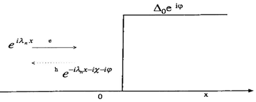
Andreev Reflection

In 1965, Andreev revealed a peculiar scattering mechanism at the normal- superconductor interfaces caused by a sharp spatial variation of gap parameter. An incoming electron of energy below the gap, incident on the superconducting interface reflects back as a hole of opposite spin, as a result of which a Cooper pair is injected into the superconducting region. In the same manner a quasi­ hole is reflected as a quasi-electron while absorbing a cooper pair from the superconducting region(Fig.

2

.

1

).

This process can be described using Bogoliubov-de Gennes equations. Consider a step like gap parameter vanishing in the normal region (a: <

0

) and of constant value Ae*^ in the superconducting region(a; > 0). The problem is

CHAPTER 2. BOGOLIUBOV-DE GENNES AND GORKOV ... 19

one dimensional, so Bogoliubov-de Gennes equations should be reduced to one dimensional form(see Chapter-3). The incident electron in the

N

region,

a: <

0

0

k, = y/2m{E + (:,J

(2.31)

Cox — C

_’

_2m

Ql

is an incoming electron with positive Fermi momentum. The reflected excitations

X

the first part of which is an outgoing electron with negative Fermi momentum, and the latter is an outgoing hole with positive Fermi momentum. The transmitted excitations for a; >

0

,

A± =

7

± = (£^ db zQ)/Ao

(2.33)

where the first part of the solution is an electron type excitation and the latter is o f hole type, being defined as follows

D

= / Ë

2

T K

2

, £; > Ao

ÇI

=

i^|^l - E^,

E < A o

CHAPTER 2. BOGOLIUBOV-DE GENNES AND GORKOV ... 20

Matching the wave functions and their derivatives at the boundary a; =

0

produce the coefficients, and

B

comes out to be of order of Aq/C^x- This means that Fermi

momentum is approximately conserved since Ao/Cgx is a very small quantity which can safely be ignored. However, this is only valid, when there’s no diagonal potential. Charging effects, or defects in the interface or in general, the existence of diagonal potentials produces diagonal scattering as well(i.e. Fermi momentum changes the sign). The conservation of crystal momentum in the lack o f diagonal ])otentials, is the motivation for the

semiclassical approximation

which will be studied in the third chapter. The underlying idea is in studying the case of negative and positive Fermi momenta independently.

For

E < Ao

the solutions yield

\A\

«

1

, on the other hand, wave functions attenuate in the superconducting region, as a result the incoming electron reflects back as a hole. This is nothing but the Andreev reflection. This reflection is not a specular one, and is called the retroreflection(Fig-

2

.

1

).

If the length of the superconducting islands in

SNS

structure (Srsuperconducting, N;Normal) is large enough, the tunneling o f Cooper pairs is suppressed and Andreev reflection becomes the prominent transport mechanism at voltages and temperatures below the gap.

/h

/'■

Figure

2

.

1

: Schematic of Andreev reflection.-Electron reflects back as a hole, then the hole reflects back as an electron at the

S

boundary, meanwhile they pick up a phase at the interfaces.

CHAPTER 2. BOGOLIUBOV-DE GENNES AND G O R K O V ... 21

2.3

Tight

Binding

Approach

and

Lattice

BogoliuboV“de Gennes Equations

The effective Hamiltonian can also be written in the tight binding model,

•fi.// = E

{(''>

-

+

H C.)

+ +

H.C)}{2.35)

i

Operators (i^l) annihilate(create) electrons on the z’th site. Cj is the onsite energy and it may take different values in the normal and superconducting regions. is the hopping amplitude and there are mainly three values it may take, in the superconducting region, normal region and at the interface. Aj is the pairing amplitude. The

V

term takes account of the normal scattering at the interface. Using the tight binding Hamiltonian a solvable model, for instance, for the N-S interface, we have

t i > 0

t"

z =

0

t' i < 0

A i > 0

0 ¿ < 0

V = VS,¿1

(2.36)

The interface is chosen to lie in between

2

= 0 and

2

=

1

. Different values of

on

normal and superconducting regions take account of the Fermi velocity mismatch. Perfect Andreev reflection can be achieved, for instance, by taking

t = t' — t".

Even for nonzero normal scattering intensity, it is possible to achieve perfect Andreev reflection by fine adjustment of the parameter The tight binding model can be extended to handle the single or periodic SNS structure.

CHAPTER 2. BOGOLIUBOV-DE GEN^ES AND GORKOV ... 22

The tight binding Hamiltonian can be diagonalized by performing the Bogoliubov transformations

= J2{Uia7a<T -

O-i'/aTa.-cr) (2.37)

By requiring the Hamiltonian be diagonal,

H e f f = Eg (2.38)

the lattice Bogoliubov-de Gennes equations are produced,

^a'^ai

—

ti,i-lUa,i-l

T

^i,i+l‘^ai+l

+

{Vi — C)Vai

+

(■(X^ai —

~ ii,i-~lVai+l

+

{Vi

— ^)uQiA*Mo (2.39)

the lattice Bdg equations can be solved for the boundaries as in the continuum model and allows fine tuning of parameters s.t. perfect Andreev refiection is received. A thorough discussion of this model and its applications and extensions are presented in [

22

]

2.4

Green’s Functions and Gorkov’s Equations

One particle Green’s function has full information o f the quasiparticle excitation spectrum, density o f states and the thermodynamic properties. Especially whenever calculation o f the current through hybrid structures is of interest. Green’s functions proved to be very useful. Space dependent Green’s functions can be employed whenever

S—N

walls exist. The Green’s functions obey Gorkov’s

CHAPTER 2. BOGOLIUBOV-DE GENNES AND GORKOV ... 23

equations, along with the off-diagonal pair potential.

2

X

2

Green’s functions are defined as follows

= - ^ T T ^ (rr)^ (rV ')^

G(

tt

,

t

'

t

')

F{

tt

,

v'r')

F

* (rr, rV ') — G (rV ', r r ) (2.40)

where ^ (r r ) is a two component field operator

^ ( r r ) = i't ( r r ) (2.41)

The field operators are in Heisenberg picture ^ ^ (r r) =

^ , ( r r ) = e ^ " ^ i ( r ) e - ^ ’· (2.42)

One should note that ^ a (r r ) is not the adjoint o f ^ „-(rr).

Using the f i e / / (2.6) the equations o f motion for the Green’s functions can be shown to be as follows

( - ^ -

-

A)^j^(r, r') = 5(r - t

')5{

t

- r')

1

CHAPTER 2. BOGOLIUBOV-DE GENNES AND G O R K O V ... 24

The ofF-diagonal potential is

A =

0

A (r)

A*(r) 0 (2.44)

Since the Hamiltonain is time independent, Green’s functions are functions of

T — r '.

Fourier transformation to frequency domain is

S„=T

x;

uj={2n+l)'ïïT

K = T

E a;=(2n+l)7rT

(2.45)

Performing the Fourier transformation of the equations o f motion, Gorkov’s equations are produced

{iuj -

-

A )g^ r, r')

=

â(r - r')â(r

-

t

')

(2.46)

which must be solved along with self consistency condition

A (r) = - P (^ (r t ) i ’ (r i )

= K r E e - “ ”J^„(r,r)

(2.47)

where

co = (2n

+ l )

7

r r imposes the Fermion statistics and

/7

—>

0

. An elaborate discussion and derivation of the Green’s function methods, Gorkov’s equations can be found in the references [28,29].

Chapter 3

Josephson Effect in Single SNS

Structure

In this chapter, we will employ quasiclassical approximation in order to reduce the order o f Gorkov equations, the idea of which is eliminating the Fermi oscillations from the Gorkov equations, thus obtaining the quasiclassical equations for the Green’s functions with the corresponding boundary conditions. These quasiclassical differential equations will be solved for the

SNS

structure exactly, and the quasiclassical Green’s functions will be obtained. Then using the current expression(3.29), the Josephson current through the single

SNS

structure will be obtained.

3.1

Gorkov Equations in One Dimension

The equations satisfied by the thermodynamic Green functions of a pure metal-superconductor system are the second order Gorkov equations differential equations.

(iw + ^ + /^)G'a;(r, r') + A(r)F^*(r, F) =

S{

t

-

F)

(-iu. + ^ + /<) i ; ( r . O - A'(r) G„(r, r') =

0

25

CHAPTER 3. JOSEPHSON EFFECT IN SINGLE SNS STRUCTURE 26

together with the self consistency conditions

A *(r) =

\'F*{

tt

'^,

tt

)

(3.2)

Here A (r) is the gap parameter of the superconductor, which becomes zero for normal metal ,

V

is the eletron-phonon coupling constant. The thermodynamic Green’s functions appearing in the Gorkov equations are defined as follows

G(

tt

,

v

'

t

')

= - <

Т’ф^{тт)ф^{т'т') >

F *(rr, r 'r ') = - <

Тф^{тт)'ф^{т'т') >

_(3.3)

which can be expressed in the frequency domain as follows

G(rr, rV )

= T

Y,

(r. r')

Un={2n-\-\)TiT

F-(rr,

r V ) = T 5 :

cjn=(2n—l)7rT

(3.4)

F*(r,r')

is the Gorkov Green’s function and vanishes for normal metal.

The single

SNS'

structure which extends in the

x

direction is translationally invariant in the x direction. So we can eliminate transversal degrees of freedom from the Gorkov equations thus obtaining one dimensional Gorkov Equations. In order to achieve this, we perform Fourier transformation to the transverse momenta space as follows

CHAPTER 3. JOSEPHSON EFFECT IN SINGLE SNS STRUCTURE 27

G U r .r ') =

(3.5)

insertion o f the Fourier transforms of Green’s functions into the Gorkov equations yields the one dimensional Gorkov equations

(iu) - Tx +

+ A(x)F*^^^{x,x') = 5{x - x')

(-iu; - Tx

+

^kJP*kj_(^>^') -

^') =

0

4

2m

(3.6)

3.1.1

Green’s Functions for the Bulk Superconductor and

Metal

We will find the solution to the one dimensional Gorkov equations(

3

.

6

)usmg the Fourier transform method. Since we are looking for solutions for the bulk metal, we can use the translational invariance of the Green’s functions

- x ' ) = l dkx

- x ' ) = I dkx

(3.7)

where kj_,

kx

are transverse and

x

components respectively. Insertion o f the above Fourier transforms into the Gorkov’s equations yields

G „ ( k ) = ‘

CHAPTER 3. JOSEPHSON EFFECT IN SINGLE SNS STRUCTURE 28

2

)r ^

¿^2

_

h y i m y

(3.8)

Now we can calculate the Green’s functions by performing the Fourier integrals

G . _ i ' ) =

1

/ ”

ik

J ± ( ± £ í i r í I Z 5 í L e f e ( « - . ' ) X ) 27rJ-oo ’ № + ( lit ^ - k ll2 m Y 1 í L V ( x - x ' ) = ^ y _

dk.

A · _^iA:x(x-a;') oo Í

22

4

- _

kll2rny

(3.9)

where + Aq . Now we are just left with evaluating the integrals using the method o f residues. The integrands are peaked at

kx

= =FP) where

p

=

y/2mpZ, so

we can switch to integration variable k s.t.

k = K^p.

We can approximate

px_ - k'^/2m

by

±vn {v = ^2pj_/m

is the Fermi velocity in the

x

direction). After this simplification the Fourier integrals become

1

1

f°° j {—ioJ

+ u/i)e'^ p

+

r

){

x x

')

4

-(vK + ifl)-(vK — iQ)

p * U :r'\ - ^ r

X ) -

27r7_co

{vK

+

iCl){vK —

iQ) (3.10)

Making use o f the method o f residues, one can easily evaluate the above integrals and obtain the Green’s functions for the bulk superconductor,

—z G ^ k^(x,x') - ^Jkx(^.^') = ^ c o s p | x - r r '| e " ? - Q l x - x ' l

e VI

I

(3.11)

3.2

Introduction

of

Quasiclassical

Green’s

Functions

In principle Gorkov equations(3.6) can be solved for any pure superconductor- rnctal system and the Green’s functions can be obtained. However in practice, solving the Gorkov equations even for the single

SNS'

structure , since the Gorkov equations are of second order, is quite a clumsy jo b . Luckily there is a way out. It is possible to separate the Fermi oscillations from the Gorkov equations which ends with the Quasiclassical Green’s functions satisfying the Quasiclassical equations. We can predict the form o f the quasiclassical Green’s functions making use of the form o f the Green’s functions o f the bulk normal metal and superconductor with constant gap parameter (3.11). In the Green’s functions, the superconductivity manifests itself in the terms which are free from Fermi oscillations. So we expect terms to be unaffected by the phenomena related with superconductivity. This can be rigorously proven by examining the expansion of the Green’s functions in terms of the quasiparticle eigenstates of the system.

CHAPTER 3. JOSEPHSON EFFECT IN SINGLE SNS STRUCTURE 29

(3.12)

now we can express the eigenstates in the semiclassical form (see Chap.4)

'^an

(^)

Van{x)

CHAPTER 3. JOSEPHSON EFFECT IN SINGLE SNS STRUCTURE 30

where

p = y/‘2m/j,kj_

is Fermi momentum in the

x

direction, insertion of these eigenstates into (

3

.

12

) leads to the form,

G^(x,x')

= 71(7 .

—an{^

)

iuj

^an

**

1

~

^ —an

Van{x)u*^{x')

U*_^^{x)v^^n{x')'

Jcrp{x-x')

^i(Tp(x — x') na .

iuj — E„

ioj

+

E—B

(3.14)

where

a

= =Fl· So we can introduce the quasiclassical Green’s functions in the following form

(7

F:^.м,==') =

■

(3.15)

i?wkx(^)^0)/wkx*(^)^0 quasiclassical Green’s functions. However, from now on, for simplicity, we will drop the k^. We used e»<^pk-®'i instead of

^iap{x-x')

is a more familiar form from the Green’s functions we obtained for the bulk superconductor(3.11). Now we will insert the above quasiclassical forms into the one dimensional Gorkov equations(

3

.

6

) and and try to obtain the equations satisfied by the quasiclassical Green’s functions. Substitution of quasiclassical forms o f Green’s functions(3.15) into the Gorkov equations yields

^ gto-p|x-x'| I ^ _|_

2

crusgn(a: —

x')dx

+ )

gl¡{x, x')

(3.16)

S i

E

( — iw + iavS{x — x') + iavsgn(x — x')dx + ^ ) fú'^{x, x')

^

/iTTi

-á * {x )g l,{x ,x '))

=

0

.

CHAPTER 3. JOSEPHSON EFFECT IN SINGLE SNS STRUCTURE 31

Kow we will simplify the above equations. There are terms with factors

exp{iap\x —

x'|} which are fast oscillating terms compared with the other functions. We can take the coefficients of these terms to be separately equal to z('io for

X ^ x'

(i.e. when

5

Dirac function vanishes). For

x ^ x' dxsgn{x—x') —

2d(x — x')

vanishes. Here a simplification can be made, we can safely take

1

ivsgn(x - x')dxg^

>

iv s ^ {x - x')dxf*‘'

>

■

(3.17)

So we can just discard the second order derivatives for a: in the expressions (3.16).

After making the simplifications, for

x ^ x',

we re left with the quasiclassical eq u a tion s

(iuj

+

iavsgn{x - x')dx)g^

+ A (a :)/* ‘" =

0

{ - i u + iavsgn{x - x')dx)f*‘^ - N*{x)g^ =

0

. (3.18)

V

is the Fermi velocity in the

x

direction. The above equations should be solved with the appropriate boundary conditions.

Now what remains is to derive the boundary conditions either beginning from the original Gorkov equations, or using the expression (3.16) directly.

In order that the second derivatives in the expression (3.16) exist, the boundary conditions at any point

x = y

should be as follows

cr

CHAPTER 3. JOSEPHSON EFFECT IN SINGLE SNS STRUCTURE 32

where

e

—>· O'··. Since are fast oscillating terms, the coefficients of

(.’<^p{y-x')

can separately be taken to be zero. So these lead to the continuity o f quasiclassical Green’s functions conditions at any point

x,

{x

+ e,

2

;')

- g ^ { x -

e,

x') =

0

/^+(a; + e,

x') - f*~(x - e , x ' ) = 0 .

(3.20)

The further boundary conditions are obtained by integrating(3.16) in the interval

(y — e,y + e)

for

y ^ x',

leads to the trivial condition 0 = 0. For the case

y = x'

the integration in

{x' — e,x' + e)

interval yields the normalization

9^ W , ^') - 9uj

f;^{x',x') - f~ {x',x')

= 0

(3.21)

We obtained the equations o f motion for the quasiclassical Green’s functions and the corresponding boundary conditions. The quasiclassical equations are of first order which are easy to handle. Their simplicity will be made clear when the quasiclassical equations are applied to the bulk superconductor with constant gap parameter.

3.2.1

Application of the Quasiclassical Equations to the

Bulk Superconductor with Constant Phase

The quasiclassical Green’s functions will be obtained for the bulk superconductor by solving the quasiclassical equations with the boundary conditions and compared to the ones obtained directly from the Gorkov equations(3.11). We will solve the quasiclassical equations (3.18)for the bulk superconductor with a constant gap parameter A = Aoe*^ , then we will impose the boundary conditions( 3.20, 3.21). The solution set for quasiclassical equations (3.18) is given as

CHAPTER 3. JOSEPHSON EFFECT IN SINGLE SNS STRUCTURE 33

s: « I

I e*“

Sc oc TTe-¿x =

- i

,

6

t; ± sgn(a; —

x')

Ao

Ü

V « = - go; = _f*0 J (jj (3.22)

X is the phase of the superconductor.

We can choose for

x'

any value we wish, due to translational invariance of the system. Suppose we choose

x'

= 0.

For

2

; < 0, 7

6

*^ 7+e (3.23) for

2

; >

0

, 7

6

*^ go; = ^ 7+g

IX

7^ =

—i

w ± A,

₀

(3.24)

The above solutions are introduced such that they vanish at infinities. Imposing the boundary conditions at the point

x = 0

given by (3.20,3.21) we can determine the coefficients.

C - A = 0

B - D = 0

CHAPTER 3. JOSEPHSON EFFECT IN SINGLE SNS STRUCTURE 34

A — B — —i/v

A-f- -

B

7

+ =

0

(3.25) The above equation set can easily be solved and the final solution for the full Green’s functions for the bulk superconductor are as follows

A*

=

--- e

2vn

(3.26)

Then the full Green’s functions for the bulk superconductor of constant phase, are as follows

G ^ x) = ^

( ^ + l)e ’>l^l + ( ^ - l)e-'P l’'l

(3.27)

So using the quasiclassical equations we were able to obtain the Green’s functions for the bulk superconductor correctly(3.11). Just by taking Aq -> 0 we can obtain the Green’s functions for the bulk normal metal

Guix)

=

[(sgncu + l)e*^l®l + (sgnw - l)e

e

3.3

Calculation

of the

Josephson

Current

Through a Single SNS structure

The expression for the current through a single

SNS'

structure is given by the following expression

CHAPTER 3. JOSEPHSON EFFECT IN SINGLE SNS STRUCTURE 35

(27t) xeS' Jx’ eS

-

i

f

)d x d x ''£ A {x )A * {x ')G l^ ^ {x -x ')G -^ i,^ {x ',x )

(3.29)

JxeS Jx'eS' ,,,

6

'° (a; —

x'), Gu{x,x')

stand for the Green’s functions o f the bulk normal metal and single

SNS'

structure, respectively.

According to (3.15), the current expression (3.29) can be expressed in terms o f quasiclassical Green’s functions

CHAPTER 3. JOSEPHSON EFFECT IN SINGLE SNS STRUCTURE 36

r

C

roo

_^

{gLi^ - x')g-u;{^', x)

+ rc)} (3.30)

where we have discarded the highly oscillating terms, since their contribution is very small.

So, in order to find the Josephson current, we are just left with solving the quasiclassical Green’s functions (3.18) for

SNS'{3.1)

. We will take x ' <

0

(i.e.

x'eS)

, and write the solution for quasiclassical Green’s functions in the four regions and obtain the solution for the case

x'eS'

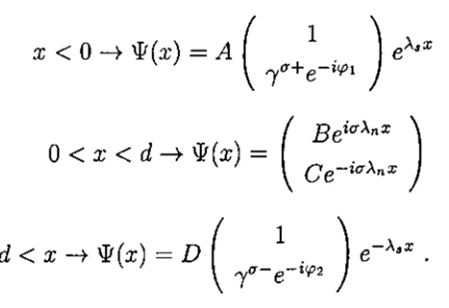
by symmetry considerations. The solution set for the superconducting region with constant phase % has been presented in (3.22). The solution set for the normal metal is

0-+ rv I ^ I ^-wa;sgn(i-®')/v / ^ I o;xsgn(x-x')/v

0

’

1

go; OC ^(jJXSgn{x-x')lv

^—LJXSgTi{x-x')lv

(3.31)

We will be writing the solutions in the four regions, for each region we will pick up the solutions s.t they vanish at infinities, if that region extends to infinity. For a:' <

0

the solutions in four regions are

CHAPTER 3. JOSEPHSON EFFECT IN SINGLE SNS STRUCTURE 37

x' < X < 0

— Cl

7'^e' +

Di

7 e'

EZ = C2{

~ .... I e- + D2

7 e

-iXl

7

+g ixi i^ie Ax

0 < x < d —^ g ^ = ,

_{go, =} C?

2

e Ax - A x

d < x ^ g ! , = H\

| e - “' Й = 7| | e -“ (3.32) 7 e /у“Ь g ^X

2

where

\ = u/v.

Here г; is the Fermi velocity in the

x

direction. Imposing the boundary conditions given by (3.20, 3.21), at x =

x'

the following boundary conditions are obtained,

(A -

C'i)e'^*' -

Die-·^^' =

0

{B -

C'

2

)e''®' - A e " ''* ' = 0

{ A j - -

C i

7

+)e''^' -

Da~e-'^^' =

0

(5 7 + - C'

27

")e''^' - 5>27+e-''^' =

0

(A - 5)e''®' = - г /v

A y - - B y+ = 0 . (3.33)

At X = 0, we apply the boundary conditions(3.20) yielding

CHAPTER 3. JOSEPHSON EFFECT IN SINGLE SNS STRUCTURE 38

C2 P D 2 ~ F2

— 0

( C 1 7 + +

- G i =

0

( C 2 7 " +

- G 2 =

0

.

At X — d , we apply the boundary conditions(3.20),

=

0

F

26

^'^ -

=

0

Gxe^^ -

^/■7- 6-''^'-'^^ = 0

G

2

e~^^ -

/ 7 + 6 - '''^ “ *^=* =

0

.

(3.34) (3.35)

The boundary conditions (3.33,3.34,3.35) can be solved thus obtaining the unknown coefficients. If we examine the current expression(3.30), we only need the quasiclassical Green’s functions

g^^{x,x'), f^ {x,x')

either

xeS, x'eS'

or

xeS\ x'eS.

In our calculations, we have taken

x'eS,

so for

xeS', x'eS

(3.32) the quasiclassical Green’s functions for

SNS'

are

V e - ^ '^ -

Re^'^+^'x-Considering the symmetry o f the problem, we can obtain the solution for

xeS', x'eS

just by the replacement

x

to

{—x

+

d)

and

x'

to

{—x'

+

d)

as well as x to ~ x .

4

./ /N ^ -«fx '-l) - / * (

2

^. ^ “ g-Ad-ix _

HgXd ^

r,Kd

V

— Re^'^

^ g - « ( x '- 0 . 3 7 )

CHAPTER 3. JOSEPHSON EFFECT IN SINGLE SNS STRUCTURE 39

Where

R = {u + ft)/{oj — LI)

and

x = Xi — X

2 is the phase difference between the two sides, A =

u/v.

The bulk metal quasiclassical Green’s functions are also needed(3.28)

—i

9

^ {x ,x ') =

— ( l + sgno;)e v

9oJx,x')

= ¿ ( 1 “ sgnw)e“ '® ^'1(3.38)

Now we are left with evaluating the current expression (3.30). Replacing =

27

rk±dk±

=

—rn^2‘Kvdv,

where

v

is the Fermi velocity in the

x

direction, and inserting the quasiclassical Green’s functions into (3.30) and performing the space integrals yields

J =

Aievn^T ^ pF ,

2

TT <3-0

-/0

1

Re>'d+ix -

Re^^

- 4 --- (3.39)

-IX —

e~^‘^ J

where oj = (

2

n +

1

)

7

tT, n = 0 ,

1

,

2

.. . This current expression can be put in a concise form

J =

8em^ A

q

,

2

TT

’ 53

_w>

₀

_‘'°

r d v v

sinx

{u +

+

2

A

0

COSX + (w -

Cl)^e

i(3 .4 0 )

From (3.39) the integrand can be written in a form suitable for series expansion.

CHAPTER 3. JOSEPHSON EFFECT IN SINGLE SNS STRUCTURE 40

J

AierrPT pF

/

d v v Y ,

e -2 \ d

o-^X

2

TT

Jo

_R

Q - 2 X d - i x R 1 -g-2Ad+tx R (3.41)

Performing the series expansion gives

J =

SerrPT rF

r

d v v Y , t e - ^ > C ‘^

y

3in{nx) .

(3.42)

Jo

^

\u + i l j

27T

First the T =

0

limit will be considered. As T ->

0

, the replacement

dn

=

doj/2'KT

can safely be done, and summation in (3.41) can be converted into an integral over frequency. To the first order in cu/fi we can make the following expansion

( ^ ) · ■ I - · ' · ! ' - T · · < " · ' « · » . (3.43)

Employing this expansion in the previous current expression(3.42) and performing the integrations, we obtain the following expression for the current at T = 0

J =

- 4 A o e ( : / “ ( -

1

) “ . , , , f o

& ,

(

2

Tr)! •

2

_{n = l}E (3.44)

There’s a summation to be evaluated

2

f ( _ i ) " + i S M ! U ) = ; ^ ( „ „ r f (

2

,r))

n = i

(3.45)

which is nothing else but the periodic sawtooth function, and from (3.44) it can be seen that Josephson current becomes independent o f Aq and its amplitude is