Large vocabulary speech recognition in noisy environments

JVRQE ypCA SU LA RY SPEECH RECOGNIflON IN

\

_{NOISY ENyiRpNMENTSi A^^^}

A THESIS

?UBM! T O

BgPARTMENT OF ELECTRiCAL· AND ELEGTRO.NiC;

'

i^NGlNEERING V

^

AND THE INSTITUTE OF ENGINEERINO'AND SCIENOES

:

OF Bil-KENT UNIVERSITY

: IN PARTIAL FULFILLMENT OF THE REQUIREMENTS

FOR THE bEGREE OF

-

MASTEFTOF oCIENeE''' -

"----Fn-eis Jablourt

July

S

?S9S

J 3 I

/9 9 S

LARGE VOCABULARY SPEECH RECOGNITION IN NOISY

ENVIRONMENTS

A THESIS

SUBMITTED TO THE DEPARTMENT OF ELECTRICAL AND ELECTRONICS ENGINEERING

AND THE INSTITUTE OF ENGINEERING AND SCIENCES OF BILKENT UNIVERSITY

IN PARTIAL FULFILLMENT OF THE REQUIREMENTS FOR THE DEGREE OF

MASTER OF SCIENCE

By

Firas Jabloun

Т/с

Л І І

11

I certify that I have read this thesis and that in my opinion it is fully adequate, in scope and in quality, as a thesis for the degree of iMaster of Science.

A. Enis Çetin, Ph. D. (Supervisor)

I certify that I have read this thesis and that in my opinion it is fully adequate, in scope and in quality, as a thesis for the degree of Master of Science.

Orhan Arikan, Ph. D.

I certify that I have read this thesis and that in my opinion it is fully adequate, in scope and in quality, as a thesis for the degree of Master of Science.

Mübeccel Demirekler, Ph. D.

Approved for the Institute of Engineering and Sciences:

. Meh

Prof. Dr. Mehmet Baray ■

ABSTRACT

LARGE VOCABULARY SPEECH RECOGNITION IN NOISY

ENVIRONMENTS

Firas Jabloun

M.S. in Electrical and Electronics Engineering

Supervisor: A. Enis Çetin, Ph. D.

July 1998

A ІКПѴ set of speech feature parameters based on multirate subband analysis and the Teager Energy Operator (TEO) is developed. The speech signal is first divided into nonuniform subbands in mel-scale using a multirate filter-bank, then the Teager ener­ gies of the subsignals are estimated. Finally, the feature vector is constructed by log- compression and inverse DOT computation. The new feature parameters (TEOCEP) have a robust speech recognition performance in car engine noise which has a low pass nature.

In this thesis, we also present some solutions to the problem of large vocabulary speech recognition. Triphone-based Hidden Markov. Models (HMM) are used to model the vocabulary words. Although the straight forward parallel search strategy gives good recognition performance, the processing time required is found to be long and imprac­ tical. Therefore another search strategy with similar performance is described. Sub­ vocabularies are developed during the training session to reduce the total number of words considered in the search process. The search is then performed in a tree structure by im^estigating one subvocabulary instead of all the words.

Keywords : Speech recognition. Multirate subband anttlysis, Teager En­ ergy Operator, Nonlinear speech modeling. Triphones, Tree structure search strategy.

ÖZET

KONUŞMA TANIMA

Firas Jabloun

Elektrik ve Elektronik Mühendisliği Bölümü Yüksek Lisans

Tez Yöneticisi; Doç. Dr. A. Enis Çetin

Temmuz 1998

.A.ltbant analizi ve Teager Enerji Operatörüne (TEO) dayal yeni bir konuşma öznitelik parametresi seti geliştirildi. Konuşma işareti önce me/skala içinde düzgün olmayan alt- bantlara bölündü. Sonra, alt-işaretlerin Teager Enerji kestirirnleri yapıldı. Son olarak log sıkıştırma ve ters DCT hesaplamasiyla öznitelik vektörleri oluşturuldu. Yeni öznitelik parametreleri (TEOCEP), döşük geçiren bir yapısı olan araba motor sesine karşı görbüz tanıma performansına sahiptir.

Bu tezde ayrica geniş kelime hazneli konuşma problemine ilişkin çözümler sunuldu. Kelimeler üçlü-fon temelli HMM ile modellendi. İşlem zamanını azaltmak için, öğrenme süresinde alt kelime hazneleri geliştirilip, ağaç yapılı arama işlemi gerçekleştirildi.

Keywords : Konuşma tanıma, altbant analizi, Teager Enerji Operatörü, doğrusal olmayan konuşma modeli, üçlü-fonler, .A.ğaç yapılı arama stratejisi.

ACKNOWLEDGMENTS

I would like to express my deep gratitude to my supervisor Dr A. Enis Çetin for his guidance, suggestions and valuable encouragement throughout the development of this thesis.

I would like to thank Dr Orhan Arikan and Dr Miibeccel Demirekler for reading and commenting on the thesis and for the honor they gave me by presiding the jury.

I am also indebted to my family for their continuous morale support throughout my graduate study.

Sincere thanks are also extended to all my friends and to Sevinç who encouraged me during the development of this thesis.

To ту family

C o n ten ts

1 Introd uction 1

2 T he speech recognition system 4

2.1 Endpoint D etectio n ... 4 2.1.1 Feature E x tr a c tio n ... 6 2.1.2 R e co g n itio n ... 6

2.1.3 Word Models 8

3 Speech P rocessing Techniques 11

3.1 Sub-band Analysis 11

3.2 Non-linear Properties of Speech S ig n als... 15

4 T he Teager Energy Operator 19

4.1 Properties of the Teager Energy Operator 19

4.2 Car N o i s e ... 21

4.3 The Cross 'F-Energy 23

4.4 Speech in car n o i s e ... 23 4.5 The TEOCEP Feature V e c to r ... 29

CONT ENTS V U l 4.6 Simulation R e s u l t s ... 30 4.7 Variations of the TEOCEP fe a tu re s... 32 4.8 C onclusion... 33

5 Large Vocabulary Speech R ecognition 34

5.1 Triphone-Based Markov M o d e ls ... 34 0.2 R e co g n itio n ... 35 5.3 The Best State S equence... 36

5.4 The Training Problem 37

5.5 The Subvocabulary Based Search S tr a te g y ... 38

5.6 Simulation Results 41

5.7 Conclusion... 42

6 C onclusion 43

A P P E N D IX 44

List o f F igu res

2.1 The speech recognition sy s te m ... 2.2 The parallel strategy recognition procedure

2.3 A five-state left to right HMM model with the feature vectors each being generated by one s t a t e ...

7

9 0

3.1 Basic block of sub-band decom position... 12

3.2 A two stage tree structure subband decomposition d e s ig n ... 13

3.3 The sub-band frequency decomposition of the speech sig n a l... 13

3.4 The tree structure sub-band decomposition... 15

4.1 Power Spectrum Density of the car noise signal

4.2 Spectrum of car noise energy <f['y(n)] (dashed line) and the spectrum of T['u(n)] (continuous l i n e ) ... 4.3 Plot of the function /(D ) = ^[3 -I- cos^(2Q) — 4cos^ fl] (continuous line),

and g{Q) = a'^sin^Q (dashed line) for Q, G [0,7t] with n = 1... 4.4 V'ar{Ti} (continuous line) and Var{^x} (dashed line) in function of 0 for

G [0,7t]. Here = 1 ... 4.5 Plot of 60 msec of the vowel / a / ...

21

22

26 26

LIST OF FIGURES

4.6

4.7

4.8

Power spectrum of the i^-energy (left) and ^-energy (right) of the vowel / a / in noise free (upper plot) and noisy (bottom plot) conditions with

SNR= OdB. 27

Power spectrum of the ^-energy (up) and \&-energy (down) of the vowel / a / in noise free (continuous line) and noisy (dashed line) conditions with SNR=0 dB. Just the first 1/10 of the spectrum is shown here.

Power spectrum of the ^-energy (up) and if-energy (down) of unvoiced phoneme / s / in noise free (continuous line) and noisy (dotted line) condi­ tions with SNR=-5 dB. The plots on the right hand side show the same spectra zoomed to the frequency range 0 Hz to 500 Hz

28

29

5.1 Cascading the HMM models of the three triphones forming the Turkish word ‘TiF to form the final word model... .36 5.2 A two stage subvocabulary search strategy... 39

List o f T ables

4.1 The average recognition rates of speaker dependent isolated word recogni­ tion system with SUBCEP and TEOCEP representations for various SNR

levels with Volvo noise recording. .31

4.2 The average recognition rates of speaker dependent isolated word recogni­ tion system with SUBCEP and TEOCEP representations for various SNR levels with white noise... 31 4.3 The average recognition rates of speaker independent isolated word recog­

nition system with SUBCEP and TEOCEP representations for various

SNR levels with Volvo noise recording. 32

4.4 The average recognition rates of speaker dependent isolated word recog­ nition system with TEOSUBl and TEOSUB2 features for various SNR

levels with Volvo noise recording. 33

5.1 The classification A lg o rith m ... 40 5.2 Recognition rates for Stock Market Database after several training sessions 41 5.3 The recognition performance : the parallel search versus the subvocabu­

lary based s e a r c h ... 42

C h ap ter 1

In tro d u ctio n

Spetich is the most efficient and natural means of communication among human beings. While this has been true since the dawn of civilization, the invention and widesprecid use of the telephone, audio-phonic storage media, radio and TV has givcni (U'cn further importance to speech communication and hence to speech processing [1,2]. Further, the way humans produce and perceive speech sounds has also become a stimulating area of research, aiming to create machines that can receive spoken informariou and act appropriately upon that information or even answer and be able to discuss [3,4]. In the world of science fiction, computers have always listened and spoken to us exactly as humans do. However, in reality, the speech technology is still not as sophisticated as the dream itself. Fortunately, the advances in digital signal processing technology brought new robust methods for both speech recognition and synthesis [5,6]. Nonetheless, the objective of a robust, intelligent, fluent conversant machines remains a distant goal.

Three mcdn areas can be distinguished in the field of speech processing, although they overlap considerably; coding, recognition and synthesis. Speech enhancement and compression are also useful for both recognition and coding. In this thesis the problem of spec'ch recognition is considered and new methods which enhance the recognition ability are introduced.

Speech recognition is a rather challenging problem whose dimensions of difficulty are usually viewed in three different ways. The size of the vocabulary can be considered as the first dimension. The performance of the recognizer usually degradf's as the vocabulary

CHAPTER 1. INTRODUCTION

size of the system increases. Speech recognition systems are generally classified with small (2-99 words), medium (100-999 words) or large (more than 1000 words) vocabularies [5].

The second dimension of difficulty is the problem of speaker dependency. A speaker dependent recognizer uses the utterances of a single speaker to train the models which characterize the system. This system, then, should be used specifically for recognizing the trainer’s speech. Accordingly, the recognizer will yield relatively high recognition rates compared with a speaker independent recognition system. The latter is trained by multiple speakers and used to recognize many speakers including those who may be outside the training population.

The most complex systems perform continuous speech recognition, i.e., the user utters the message in the most natural manner used in real life [7,8]. The difficulty here is to be able to detect the boundaries in the acoustic signal, and to perform well in spite of all the co-articulatory effects and sloppy articulation (including insertions and deletions) that accompany flowing speech. To get rid of all these difficulties, simpler systems use isolated-word recognition which is a relatively much easier problem. Pauses between words simplify the recognition process because endpoints become easier to identify in addition to minimizing the co-articulation between words. Sometime the application n ia k ('S it unnecessary to use continuous speech though achieving a high recognition rate with continuous speech stays as the ultimate goal of the speech recognition research.

Ill this thesis, the problem of large vocabulary speech recognition in noisy environ­ ments is investigated. In most cases background noise is modeled as additive stationary perturbation which is uncorrelated with the speech signal. With this assumption we con­ struct a robust speech recognition system in the presence of car noise. Applications inside automobiles have a very practical importance and that is why car noise environment is examined in this thesis.

In Chapter 2, general concepts of speech recognition are introduced. Namely, the different modules required by the speech recognition system based on a Hidden Markov Model (HMM) are reviewed.

In Chapter 3, the wavelet analysis of speech signals or equivalently the multirate subband analysis is introduced and inspected. Subband cepstral coefficients show a more robust performance for speech recognition than the commonly used mel-scale cepstral representation. Chapter 3 also introduces the nonlinear modeling of speech signals. Experimental results show the existence of important nonlinear phenomena during the

CHAPTER 1. INTRODUCTION

speech production that cannot be accounted for by the linear model [9,10]. Each speech resonance is modeled with an AM-FM modulation signal and the total speech signal as a superposition of such AM-FM signals. In [11-15] a new energy operator ('■!') was successfully used to separate the modulation energies.

In Chapter 4, the energy operator is used with a multirate subband decomposition approach. The new energy is used as a substitute for the traditional energies to benefit from its robustness against colored car noise. Experimental results show that the car noise T-energy is negligible compared to that of the speech signal, if the resonance freciuency of the latter falls within the current analysis frequency band.

A large vocabulary speech recognition system is designed in Chapter 5. A triphone based Hidden Markov Model (HMM) is used to model the phonetic content of one phoneme together with its left and right neighbors. The use of triphone subwords com­ pensate for the lack of a large training database. Furthermore, as the vocabulary size iiicreases, the recognition time becomes important since in speech recognition a fast response is necessary in order to have a practical system. A guided strategic search ai)proach is designed to reduce the effective vocabulary code book.

C h ap ter 2

T h e sp eech recogn ition sy ste m

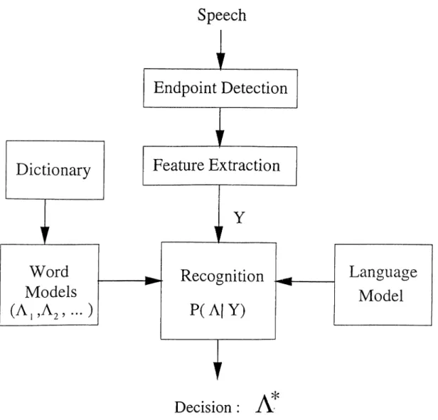
The speech recognition system consists of several modules each of which constitutes a fundamental stage for the recognition process. In the case of continuous speech, how­ ever, the endpoint detection module becomes meaningless while other more complex manipulations are performed usually during the recognition phase using tlu' word mod­ els rlu'mselves. Each of the modules shown in Figure (2) is descril:)ed below in detail.

2.1

Endpoint Detection

The endpoint detection module is an important step in the isolated word speech recogni­ tion .systems. Obviously, a robust endpoint detection algorithm contributes significantly to improve the overall performance of the recognition system . In the presence of noise (such as car noise) the traditional methods for endpoint detection which use the en­ ergy and the zero-crossing rate [16] , degrade drastically and usually fail to detect some phonemes such as the weak fricatives. Instead, an alternative measure which takes into account the statistics of the environmental noise, is used.

In this thesis, sub-band decomposition [17-19] plays a fundamental role in the acous­ tic modeling of speech, and it will be discussed in detail in Chapter .3. Nonetheless, it is introduced here since it is needed to describe the endpoint detection algorithm.

CHAPTER. 2. THE SPEECH RECOGNITION SYSTEM

Speech

Decision : A "

Figure 2.1; The speech recognition system

Suppose that a filter bank is used to decompose the speech signal into several sub­ signals each of which is associated with one of the bands in the frecpiency domain, the following energy parameter E^ is defined for the speech frame and the C'' sub-band.

1 Ni ^ 71 = 1

Consequently the distance measure used is defined as follows :

Dk — lOlofj

(2.1)

1 ^ (Et

-^ l=l

(2.2)

CHAPTER 2. THE SPEECH RECOGNITION SYSTEM

respectively. They are estimated a-priory from the utterance free segments as : 1 N k=l N (2.3) (2.4) k=l

Using this distance measure an efficient algorithm for endpoint detection can be designed arid is described in detail in [20].

2.1.1

Feature E xtraction

A fundamental assumption in most speech recognition systems is that the speech signal can be considered as stationary over an interval of a few milliseconds. This assumption is a legitimate one because the human speech production system is a physical system which can not change very quickly with time. Thus speech can be divided into frames each of which is considered as a stationary signal. The spacing between the frames is typically in the order of 10 msec, and the blocks are usually overlapping pro\'iding a longer analysis window, typically around 25 msec long. Within each of these windows, some features to characterize the given frame are computed. In literature, several parameters were used. The Linear Prediction (LP) coefficients are the earliest ones used for both speech recognition and coding [21-24]. LP coefficients do not show good performance so other features like the Line Spectral Frequencies (LSF’s) are proposed in [25- 28]. Recently, Melcep coefficients [7,29,30] and sub-band cepstrum coefficients [17-20], become the most widely used features for speech recognition. In this thesis, new features which offer robustness against noise with high recognition rates are developed and are discussed in detail in Chapter 4.

2.1.2

R eco g n itio n

After detecting the endpoints of the utterance and extracting the features from the speech signal, the recognition phase starts. Assuming that we have a model for each word in the vocabulary, we want to find the model which has the highest probability of [)roducing the given sequence of feature vectors. In other words, suppose we have a

CHAPTER. 2. THE SPEECH RECOGNITION SYSTEM

sequence of vectors Y = {yi, y2, ■ ■ ■ /yr}, where T is the total number of frames, and yi is the feature vector. A word W* is claimed to be the uttered word if

W* = ar g m a x P { A w \ Y } W

(2.5)

where Aw is the model characterizing the word W. This problem, however, is rather a difficult one. The solution is to solve the dual problem of finding the probability of having the feature vector Y given the model Aw or PlFIAvi/}· This can be achieved using the Bayesian rule [31]:

W* — arg max P { A w \ Y } = ar g m a x P{Y'\Aw}P{Aw}

W W P { V )

(2.6)

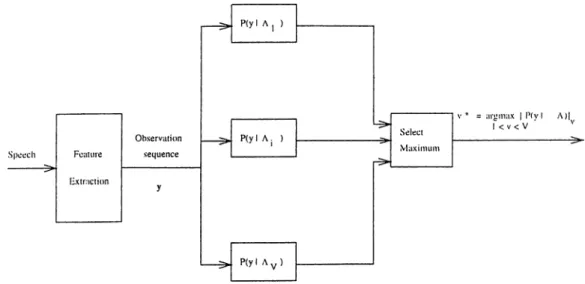
The probability F{T} is of no importance since Y is given and its probability can be considered to be one. jP{Aw} can be computed through a language model. The simplest case is to use a uniform distribution where the verification process follows a parallel strategy which includes all the words of the vocabulary as shown in Figure (2.1.2). This techniciuc. while satisfactory for small vocabularies, is not practical for medium and large vocabulary applications in which more complex search strategies must loe used.

CHAPTER 2. THE SPEECH RECOGNITION SYSTEM

2.1.3

W ord M odels

There are several methods to model the words of the dictionary. These include the neural network approach [5], a stochastic model using Hidden Markov Models (HMM’s) [5,6,32]. In this thesis, the HMM stochastic model is used.

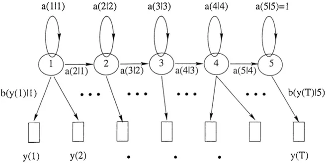
The idea is to represent a word by a finite state machine with a left to right structure as shown in Figure (2.1.3).

The HMM is assumed to generate observation sequences by jumping from state to state and emitting a feature vector upon arrival at each successive state. Each model is characterized by a set of parameters. These are the state transition probabilities

a{i\j) = F^{xt — = j} , where Xt is the state at time t (or tP'· frame). The matrix of state transition probabilities is given by

a ( l|l) a (l|5 ) A =

a (5 |l) a{S\S)

(2.7)

WIkuc S is the total number of states in the model. The state transition probabilities are assumed to be stationary in time, so that a{i\j) does not depend on the time t at which the transitions occurs. Note that any column of A must sum to unity, since it is assumed that a transition takes place with certainty at every time instant.

The state probability vector at time t is defined as

7 r ( i) =

P{x{t) = 1)

(2.8)

P{x{t) = S)

So that 7r(i) = A7r(i - 1) and by recursion 7r(i) = A(‘~^^7r(l)

Therefore the state transition matrix and the initial state probability vector, fully identify the probability of residing in any state at any time.

Upon arrival at one of the states, the model emits an observation vector y{t) with some probability

CHAPTER 2. THE SPEECH RECOGNITION SYSTEM

This probability can be discrete and computed using vector quantization from a priorly defined fixed code book. However the precision of this approach (though computationally very efficient) is very limited with the noise introduced by quantization. Therefore it is not used anymore since its continuous counterpart has shown a much better performance.

a(lll)

a(3l3)

a(5l5)=l

b(y(l)ll)

y(i)

y(2)

y(T)

Figure 2..3: A five-state left to right HMM model with the feature vectors ciach l)eing gcmerated by one state

Modern systems use parametric continuous-density output distributions that model the acoustic vector directly. This distribution together with the initial state i)iobability and the state transition matrix are necessary and sufficient to completely model the words of the vocabulary. Formally this is written as :

M = {7t(1), A,/y|a;(C|a;) ; 1 < (2.10) Usually fy\:rXC\x) is chosen to be a multivariate mixture normal distribution [.3.3], that is a linear combination of Gaussian pdf’s :

M

fy\x{C\'^' — 'i') — ^mi ^rni)

rn=l

(2.11)

Where Cmi, and Cmi are the weight, mean vector and covariance matrix, respec­ tively, of the distribution of the C’' state. Note that ('„u = i all / = 1 ,... 5.

CHAPTER 2. THE SPEECH RECOGNITION SYSTEM 10

This stochastic model presents three major problems which shall be solved. These three problems are the recognition, training and the state sequence followed. Fortunately in literature several algorithms to solve these problems were used, the most widely used are the Forward-Backward [5,6,34,35] algorithm and the Viterbi algorithm [5,6,36-38]. While the first method can only calculate the likelihood P{y\A) regardless of the path followed, the second one tries to calculate the same likelihood through the best path and thus provides information about the best state sequence. In this thesis, the Viterbi algorithm was used in for recognition while a mixture of both approaches was used for training.

C h ap ter 3

S p eech P ro cessin g T echniques

In this chapter, the wavelet analysis associated with a sub-band decomposition technique is introduced. The subband analysis decomposes the frequency domain of the speech signal into several subsignals. The average energy of each snbsignal is computed. The final feature vector is obtained by applying the log compression and the cosine transform to these energies. In Section (3.2) a new energy measure which accounts for the nonlinear characteristics of the speech signal, is presented.

3.1

Sub-band Analysis

Many speech recognition systems use the rnel-frequency cepstral coefficients (M F C C 's) as features to characterize the speech signal [7,29,30]. Briefly, the MFCC's are computed l)y smoothing the Fourier transform spectrum by integrating the spectral coefficients within triangular bins arranged on a non-linear scale called the mel-scale. This scale tries to imitate the frequency resolution of the human auditory system which is linear up to Ikllz and logarithmic thereafter. In order to make the statistics of the estimated speech I)ower spectrum approximately Gaussian, log compression is applied to the filter bank output. Finally, the Discrete Cosine Transform (DCT) is applied in order to compress the sp(!ctral information into the lower-order coefficients. Moreover the DCT d(-;-c:orrelates th ('S (' coidflcients allowing the subsequent statistical modeling to use diagonal covariance

CHAPTER 3. SPEECH PROCESSING TECHNIQUES 12

matrices.

Obviously, this approach operates on the frequency domain which can be a computa­ tionally costly task. Therefore the wavelet analysis associated with a sub-band decom­ position technique was proposed and was widely discussed in literature [17,20,39-42]. It provides a fast structure for decomposing the frequency domain along with the tem­ poral information. The implementation of a wavelet transform can differ according to the application, but the easiest seems to be the tree structure which uses a single basic building block repeatedly until the desired decomposition is accomplished.

s[n]

s, [n]

sjn ]

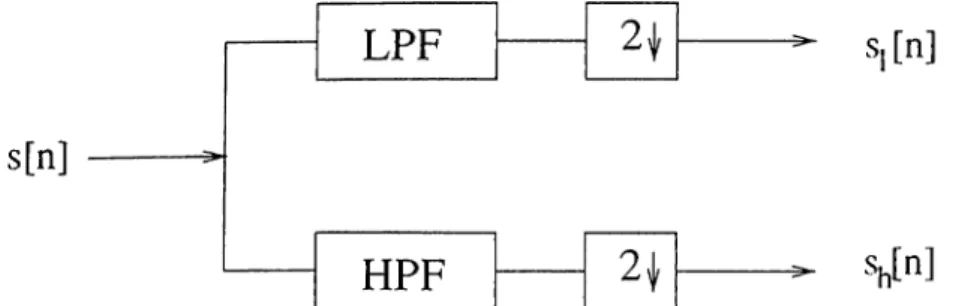
Figure 3.1: Basic block of sub-band decomposition

This basic unit uses techniques of multi-rate signal processing and consists of a low and a higli pass filter followed by a down-sampling unit Figure 3.1. The pas.s-bands of the low and high pass filters are [0, 7r / 2] and [7r/2,7r], respectively. These two filters divide the frequency range into two half-bands and the down-sampling units reduces the lengths of the obtained signals by two which consequently reduces the computational cost. Each of the sub-signals Si[n] and Sh.[n] can be further decomposed into two new

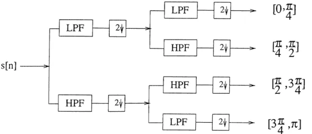
sub-signals using the same filter bank once more, and this procedure can be repeated until the desired frequency decomposition is achieved, tiere it is worth mentioning that the process of high-pass filtering and down-sampling inverts the frequency spectrum [40]. Thus while further decomposing the high-pass sub-signals, the low-pass and high-pass filters must be switched in order to get the designed frequency decomposition as shown in Figure (3.2).

These sub-signals make up the so-called wave-packet representation uniquely char­ acterizing the original signal [39]. Perfect reconstruction can be achieved with a proper choice of the low-pass and high pass filters [43]. This sub-band analysis was recentty I)ropos(;'d for speech coding purposes where it produces satisfactory results [44].

CHAPTER. 3. SPEECH PROCESSING TECHNIQUES ₁₃

S[n]

[0>J]

[ J f ]

[3 J ,7t]

Figure 3.2: A two stage tree structure subband decomposition design

It is shown in [17, 20] that the use of a sub-band decomposition filter bank corre­ sponding to a biorthogonal wavelet transform [43,45] (rather than an orthogonal one) offers better results for speech recognition purposes especially for speech contaminated with noise. One of the possible choices for the low-pass filter is the 7'^' order Lagrange filter having the transfer function

The corresponding high-pass filter has the transfer function

= 1 - | ( z - ‘ + z‘) + + e>.

(3.1)

(3.2)

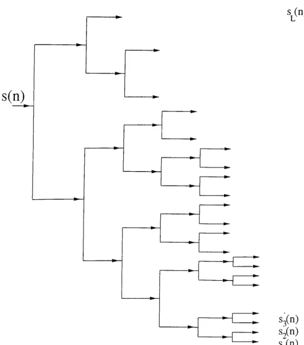
For simulation purposes, the speech signal, s(n), is decomposed into L = 21 sub­ signals, {.s/(77,)}[li using the tree structured filter bank. Figure 3.4. The corresponding freciuency domain decomposition is similar to the mel-scale [30] described above and shown in Figure 3.1.

- L . J Lj- L . 1 1 L

-*’ I kHz 2kHz

Figure 3.3: The sub-band frequency decomposition of the speech signal

CHAPTER 3. SPEECH PROCESSING TECHNIQUES ₁₄

parameters. For each sub-signal, an energy parameter e/ is defined

; 1 = 1 , . . . , L

1

= l^iNI

n=l (3.3)

where Ni is the number of samples in the band. Note that each of the parameters is defined over a finite size window of length W and overlap T. Log compression and DCT transformation is then applied to obtain the sub-band cepstrum coefficients or SUBCEP’s ;

5C■W = ¿ lo g ( e ,) c o s [ h Ц ^ : ^ L ) .

¿=1 ^

where N is the number of coefficients considered (yV = 12).

1 , . . . , N . (3.4)

In [17,20] instead of the Log compression the sub-band cepstral parameters are defined as root-cepstral coefficients [46] as follows,

SC{k) = ¿ ( e ,) » ' cos[-'=<' l=i

Ah

L k = 1, N. (3.5) Pi is the root value for the p'" band, with each band being properly weighted according

to the choice ofp/ values. This increases the robustness of the speech feature parameters in case of speech contaminated with colored environmental noise [20]. For instance, for spe.i'ch recognition under automobile noise, it is observed that the car noise has very little high frequency content. Therefore lower root values are used for the Hrst two bands. In [20] the following root values were used

P = [pxP2 ■■■ Pl]

= [0.094 0.281 0..375 0.375 ... 0.375]

(3.6)

However, the spectrum of the speech signal itself may have important information in these same lower bands, so the recognition rate may degrade with bad choices of the root values.

Usually, each acoustic vector is supposed to be uncorrelated with its neighbors. How­ ever this is a rather poor assumption since the physical constraint of the human vocal system ensures that there is continuity between successive spectral estimates [7]. Thus appending the first-order differentials to the initial feature vector will greatly reduce the problem. So if the first 12 subcepstrum coefficients are taken with additional 12 coef­ ficients from the derivative, a final feature vector with dimension 24 is obtained and is used for training and recognition.

CHAPTER 3. SPEECH PROCESSING TECHNIQUES ₁₅

s¿n)

s(n)

s7(n)

Figure 3.4: The tree structure sub-band decomposition

3.2 Non-linear Properties of Speech Signals

In speech processing, the vocal tract is traditionally modeled by a linear hlter. The actual non-linear characteristics of speech production are approximated by the standard assumptions of linear acoustics and the 1-D plane wave propagation of the sound in tlu' \'ocal tract. The well-known linear prediction model had some success in scweral

CHAPTER. 3. SPEECH PROCESSING TECHNIQUES 16

applications such as speech coding, recognition and synthesis. However, it was proven both theoretically and experimentally that there exist important non-linear phenomena during the speech production process which cannot be accounted for by the linear model [9,10].

One of the non-linear properties that has been proven to characterize the human speech production is the existence of some kind of amplitude modulation (AM) and frequency modulation (FM ) in speech resonance signals. This fact makes the amplitude and resonance frequency vary instantaneously within one pitch period [12,14]. Here speech resonances loosely refer to the oscillator systems formed by local cavities of the vocal tract emphasizing certain frequencies and de-emphasizing others during speech production. In linear speech modeling, speech resonances, also called formants, are characterized by the poles of the transfer function of the linear filter modeling the vocal tract.

Motivated by these and other evidences, Maragos, Quatieri and Kaiser [11,12,14] proposed to model each speech resonance with an AM-FM signal

x{t) = a{t) cos[f/)(i)] = a{t) cos] / и{т)(І,т -f- </i)(0)] (.3.7)

J

0

wli{'i(! a{t) and ф{і) are the instantaneous amplitude and instantaneous frequency re- s])ectively and w{t) = d(p{t)/dt. The total speech signal is assumed to Ire a superposition of such AM-FM signals, one for each formant. This approach starts by isolating indi­ vidual resonances by bandpass filtering the speech signal around its formants. Next, the amplitude and frequency signals are to be estimated based on an “energy tracking" operator. Teager has developed several tools for non-linear speech processing [10] such as the continuous time energy operator

Ф.[і(()| =

i(í)í(í)

(

-

)

If .г(п) is a sampled version of a continuous-time signal then the discrete version of the Teager Energy Operator (TEO) is obtained by approximating derivatives .i; with the 2-sample backward (or forward) difference [a:(n) - x{n — 1)]/T where T is the sampling period. W ithout any loss of generality, T can be set to one which is the case for signals initially defined in a discrete context. Then the continuous-time energy operator reduces (up to one sample shift) to the following discrete version

CHAPTER. 3. SPEECH PROCESSING TECHNIQUES 17

Both 'I'c and are nonlinear and translation invariant and were shown to track the energy of simple harmonic oscillators. Namely, if x{t) = Acos{wct + 6) then

(3.10) The idea that T is an energy measure was motivated by the fact that an undamped oscillator consisting of a mass m and a spring of constant k has a displacement x{t) = -4cos(c<;()i + 9), with uq = ^ k / m . The instantaneous energy Eq of this undamped

oscillator is the sum of its kinetic and potential energies and equals the constant

^ . 4 9

Ец = — {Auq) (3.11) Thus the energy of the linear oscillator is proportional to ^(.•[^'■(i)] in Equation (3.10).

This result can also be observed using the discrete Ф operator. Let - .4 cos(iln + ф), where is the digital frequency in radians/sample and is given by f2 = 27г///, where / is the analog frequency and fs is the sampling frequency, ф is an arbitrary initial phase in radians. To calculate the discrete Teager Energy of this sequence, three adjaccnit ecjually spaced samples of Xn are given

(З.Г2)

(3.13) .7; (n ) = Acos{0.n + Ф)

x{n + 1 ) = ^cos[i2(n + 1) + Ф] x{n — 1) = Acos[Q(n — 1) + Ф]

using the last two samples with the appropriate trigonometric identities

x{n + l):r(n - 1) = f [cos(2i2n + 2ф) + cos(2í2)]

= cos^(Qn + 0) — siii"(íí)

Notice that the first term of the right-hand side of the jjrevious equation is simply Xn squared so

Фсг[т;(тг)] = x{n Ч- l)x{n — 1) — x'^{n) = A^ siiv^(i2) (3.14) Though the result is not proportional to (AO)^, this result is still an interesting one and can easily lead to solve for .4 and Q. Moreover, for small values of ÍL sin(il) л; 0, and then

^Vd[x{n)]^A^O^ (3.15) The TEO has some useful properties which are worth mentioning at this stage

CHAPTER 3. SPEECH PROCESSING TECHNIQUES 18

The discrete version also has a similar propertj'^

Trf[x(n)y(n)] = x ‘^{n)^d[y{n)] + ?/{п)Фгі[а:(п)] - Я>а[х{п)]'І/а[у{п)] (3.17)

Now using this property and applying the TEO to a general real-valued AM signal

x{t) = a{t)cos{(jJct + Ѳ) (3.18) we have

T[a;(i)] = -I- cos^{ujct + ^)T[a(t)]

D{t) E{t)

(3.19)

Note th at no subscript was used with T since from now on both subscripts c and d will be dropped as it will be clear from the context whether the continuous or discrete-time T is used.

Here we are interested in the envelope contained in D{f) so E{t) is viewed as an error term. If a{t) is band limited with highest frequency such that < < w,.. then the error term E{t) will be negligible [13]. So Equation (3.19) becomes ^[.^(i)] a-{t)uj'f,

which has the same form as when a{t) is constant.

All the above examples provide some motivation to the use of the Teager Energy Operator in nonlinear speech processing. An Energy Separation Algorithm (ESA) was developed to demodulate the signal by tracking the physical energy implicit in the source producing the observed acoustic resonance signal and separating it into amplitude and frequency components [11,13, Id]· In this case w{t) and a{t) can be estimated as follows

w{t)

\

Simulation results show that the ESA performs pretty well and thus suggests that the Teager Energy Operator Ф “contains” useful information about the speech signal. This is subject to modeling speech resonances as a superposition of AM-FM sigricils instead of the usual approach were the speech resonances are viewed as the poles of the transfer function of the linear model of the vocal tract. The information embedded in the Teager Energy Operator (TEO) can potentially outperform the traditional energy measures used in some speech recognition applications. In Chapter 4, we will use the TEO in sub-bands and construct feature vectors based on the Ф-energy measure.

C h ap ter 4

T h e Teager E nergy O perator

In this chapter, a new set of feature parameters for speech recognition is presented. The new feature set is obtained from the cepstral coefficients derived from the wavelet analysis of the speech signal or equivalently the multirate sub-band analysis. While in [17,20] an ordinary energy measure is used to compute the cepstral coefficients, in this chapter a new energy measure based on the Teager Energy Operator (TEO) is described.

The performance of the new feature representation is compared to the Sub-band Cep- stral coefficients (SUBCEP) in the presence of car noise. The new features are observed to be more robust than the SUBCEP parameters which were shown to outperform the commonly employed MELCEP representation [17,20].

4.1

Properties of the Teager Energy Operator

As was mentioned in Section (3.2) the TEO is an efficient tool for nonlinear speech processing as long as the speech resonances are modeled as a superposition of AM-FM signals. In this chapter more attention will be paid to the discrete version of the TEO

Ф[а;(п)] = x'^{n) — x{n + l)x{n — 1). (4.1)

Clearly, this operator makes successive samples exchange information between each other inst(^ad of being treated independently as in the commonly used instantaneous energy

CHAPTER 4. THE TEAGER ENERGY OPERATOR 20

i^[.x(n)] = Moreover, as will be discussed later, the Ф-energy of the colored noise is negligible compared to that of the speech signal (especially in voiced frames) which makes it very efficient for speech recognition in noisy environments.

To be able to examine the properties of the TEO we calculate its mean, variance and the autocorrelation function in terms of the statistics of the original signal. Taking the expectation of Ф[х(п)] or simply Фі(п)

(4.2)

(4.3) E{ir^(n)} = E { x ^ n ) } ~ E {x{n + l ) x { n - l ) }

= R ^ {0 )-R ^ {2 )

where Rx{k) is the autocorrelation function of x(n) defined by

Rx{k) — E {x{n + k)x{n)}

Similarly the autocorrelation function R^{k) can be found

Ryj,{k) = E{'4/{n +

— E {x^ (n + A;)x^ (n)}

— E{x'^{n + k)x{n + l)x{n — 1)} — E { x ‘^{n)x{n + k + l)x{n + k — 1)}

+ E {x{n + l)x{n - l)x{n + k + l)x{n + k — 1)}

To simplify the above equation we assume that x(n) is a zero mean WSS jointly Gaussian random process. Hence using the Isseriis formula [31,47] and after some com­ putation Rxp^ (k) is found to be

(4.4)

(4.5)

R^vAk) = [Д^(0) + Rl{2) - 2RA0)Rx{2)]

- 4Rx{k - l)Rx{k + 1)] + [3i?2(A:) + Rx{k + 2)R,Ak - 2)

Consequently, the variance of Фі(А:) is

CHAPTER. 4. THE TEAGER ENERGY OPERATOR ₂₁

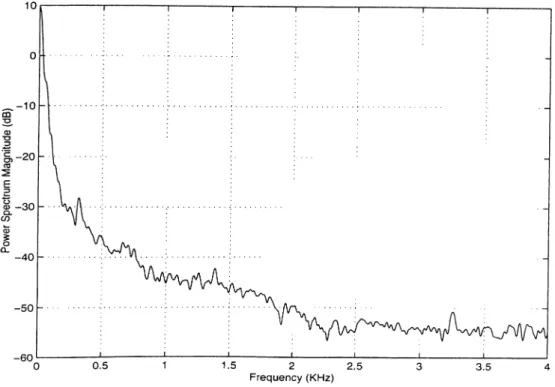
Figure 4.1: Power Spectrum Density of the car noise signal

4.2

Car Noise

Speech recognition applications inside a car can be important especially after the huge developments of the cellular mobile telephones. For instance, due to security recisons, voic(>. dialing applications can be of great interest. Nonetheless, the noise coining from the car engine will greatly degrade the recognition performance unless perfectly handled in the initial system design.

The car noise is a colored noise were its spectrum is mostly concentrated in low frequencies as shown in Figure (4.1). Thus, its correlation function varies very smoothly and it is almost flat near the origin for several lags. Consequently, with little error, we can assume that Rv{0) i?v(l) ~ Rv{‘^)· Experimental results show that

R,{1) = 0.9997 i?„(0) Ry{2) = 0.9991 R^{0)

(4.7)

CHAPTER 4. THE TEAGER ENERGY OPERATOR ₂₂

Figure 4.2: Spectrum of car noise energy ^[u(n)] (dashed line) and the spectrum of \E'[w(n)] (continuous line)

On the other hand for a speech signal s(n) of the vowel / a /, we have

Rs{l) = 0.7415 R,{0) Rs{2) = 0.4584 /?,.(0)

For this property, the mean and variance of the i^'-energy of the noise signal

(4.8)

^;{Ф„(п)} = R ^ { 0 )-R ^ (2 )

1/аг{Ф,(п)} = 3Rl(0) - 4RI{1) + Е:і і2)

(4.9)

are negligible compared to the speech signal, if the resonance frequency of the latter falls within the frequency range of the current analysis band [12]. This property is experimentally verified using several noise recordings. In Figure (4.2), it can be seen that the high level of the Power Spectrum Density (PSD) in the Іолѵ frequency rtinges of the car noise is sustained by the PSD of ^[u(n)] whereas the TEO canceled it out and thus the PSD of Ф[г’(п)] has an almost constant low level for the entire frequency range.

CHAPTER 4. THE TEAGER ENERGY OPERATOR ₂₃

4.3 The Cross 4^-Energy

Let x{n) and y(n) be two discrete signals, their cross 'L-energy is defined as

^[x{n),y{n)] = x{n)y{n) - i[x (n + l)y(n - 1) + x{n - l)y{n + 1)] (4.10) Obviously we have ’$'[a:(n),a;(n)] = 'L[x(n)]^[x(n),x(n)].

Noting th at the cross-correlation function of x{n) and y{n), which are supposed to be jointly VVSS, is Rxy(k) = E {x{n + k)y{n)}, we can study the statistics of the cross 'I'-eriergy.

The expected value of ^[x{n),y{n)\ is

E {^[x{n), y{n)]} = R^y{0) - Rxy{2) (4.11) and the variance is

V a r { ^ x in ),y { n )] } - |[3i?,(0)i?.,(0) - 4R ,{l)R y{l) + Rx{2)R,{2)]

+ ¡[3R%iO) - 4RI^{1) + R:i,^{2)]

(4.12)

Note that if x{n) and y{n) were independent and zero mean then we would have

£{Ф[х(п),у(п)]} = 0 (4.13)

Соѵ{Ф[х(гі)], Ф[х(п),у(п)]} = Соѵ{Ф[у(п)],Ф[х(п),у(п)]} = о (4.14)

The reason for defining this operator is just to facilitate the analysis as it does not have an important physical significance. Namely, it helps handling the cross terms in the computation of the Ф energy of the sum of two signals because of the nonlinearity of the TEO. This energy is found to be

Ф[х(п) -b y{n)] = Ф[х(п)] + Щу{п)] -Ь 2Ф[.х(п), у{п)] (4.15) More properties of the cross Ф-energy are discussed in Appendix A.

4.4 Speech in car noise

Now suppose that x{n) = s{n) +v{n) where s(n) is the noise free speech signal and v(n) is a colored zero mean additive noise (car noise for instance). Since v(n) and .s(n) are

CHAPTER 4. THE TEAGER ENERGY OPERATOR. ₂₄

(4.16) supposed to be independent, the autocorrelation function of x{n) is

Rx(k) = Rs{k) + R,{k)

Now since

^ [2;(n)] = ’I'[s(n)] + + 2’^[.s(n), v{n)] (4.17)

then bcised on the assumptions discussed in Section (4.2) about the car noise, and using the properties of the and cross-'i energies, we have

^{'lr,(n )} = £;{'ir,(n)} + ^{xp,(n)}

(4.18)

Equation (4.18) shows that the noise bias is negligible. Similarly, the variance of 4/[x(n)] is

V'ar { Ф } = Var{'4> s} + Var{'^]fy} + 4 Var { Ф [.s, w]}

(ЗД^(О) + Щ{2) - 4л;(1)|

+ [зя;(

) + д;(

) - «j(i)|

+ 2[ЗД.(0)Л.,{0) + R,(2)R,(2) - 4Й ,(1)Л.(І))

(4Л9)

The hrst term of Equation (4.19) is related to the speech signal. The second term, would be negligible as discussed in the previous section and can be considered as a small error term. However the cross terms at the end which are due to the noidiuear nature of the TEO, do not cancel out. Their effect, however, is reduced compared to the case when ■^[•X’(n)] is used.

The expected value and variance of <^x(n) = .x^(n) are as follows

E;{e.(n)} = Д,(0) = Rs(0) + R M (4.20)

V a r { U n )} = ЗЛ^(О) = 3(й?(0) + Rl(0) + 2Д,(0)Л„(0)) (4.21) As the noise energy increases so does the total energy of the feature parameter which is not a desirable phenomenon because it reduces the recognition quality.

This result can be checked by considering a simple example. Since we use a hlter bank which divides the speech signal into narrowbands we can assume that there is only one formant within one band and consequently the noise free speech signal n{n) can be assumed to be of the following simple form:

CHAPTER, 4. THE TEAGER ENERGY OPERATOR ₂₅

Figure 4.3: Plot of the function f{Q ) = ^[3 + cos^(2Q) -4 co s^ f)] (continuous line), and

g{i1) = sin^ 0 (dashed line) for 0. G [0, tt] with a = 1.

where G [0,7t] and a are a constant amplitude and frequency, respectively. The parameter 0 is a random phase with a uniform distribution, 9 ~ W[—tt,-]. Thus we have Rs{k) — ^cos(Qfc). Consequently,

= α^sin^í2

Var{'^s} — x[3 + cos~(2fi) - 4 cos'- fi]

(4.23)

The curves of and V^ar{\&,,} are shown in Figure (4.3) a.s a function of for

a = 1. Both functions have a bell-shaped curve with a wide band-width.

Now consider a noisy signal .■r(n) = .s(n) + v{n) so we have

it[s(n) + v{n)] — i'[s(n)] -F ’I'[u(n)] -f 2T[.s(n), v{n)] (4.24)

where v{n) is a zero mean car noise having the properties discussed in Section (4.2). Let us select E{v^{n)} = and a = \/2cr in order to make the signal to noise ratio be SNR = 0 dB. Also, assume that Rv{2) i?„(l) ~ Rv{C) = a~. As discussed in previous sections of this chapter.

¿;{^[s(n),u(n)]} = 0 (4.25)

and

(4.26) so that

CHAPTER 4. THE TEAGER ENERGY OPERATOR ₂₆

Figure 4.4; ’Far{^Fi} (continuous line) and Var{^^} (dashed line) in function of O for

Q € [0, 7t]. Here = 1 For the variance we have

V ar{'^x} Var{'^is} + 4Var{^f[s{n),v{n)}

= cr'‘[6 + (cos^(2i7) + cos(2ii)) - 4(cos'- fi + cos fi)]

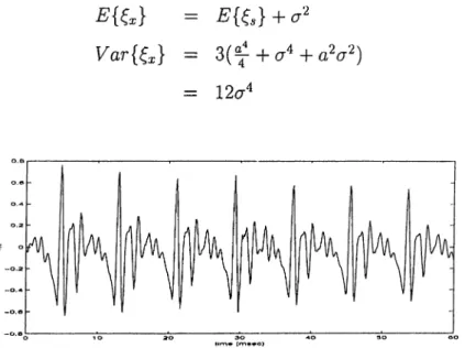
Similarly for ^{.s(n) + v{n)} E m V a r m = E { Q + a ^ — + cr‘^ + o?a'^) = 12(7'* (4.28) (4.29)

Figure 4.5: Plot of 60 msec of the vowel / a /

From Figure (4.4) it can be seen that the variance of \E',.c is smaller than that of

CHAPTER 4. THE TEAGER ENERGY OPERATOR ₂₇

frequency bands were the noise energy is mostly concentrated as shown in Figure (4.2). At O.Ttt angular frequency the variance of starts to exceed that of However at this frequency the speech formants have a relatively low amplitude for most of the phonemes and they usually do not have a significant influence on the discrimination between the phonemes [5,6]. In the case of the colored car noise, the noise power is negligible at such high frequencies. It can also be noticed that has a bias term proportional to the noise energy whereas this is not the case for ^[a;(n)].

Figure 4.6: Power spectrum of the 4^-energy (left) and ^-energy (right) of the vowel / a / in noi.se free (upper plot) and noisy (bottom plot) conditions with SNR= OdB.

To verify this result for a real speech signal, the spectrum of T[,s(n)], where s{n) is a noise free recording of the vowel / a /, is shown in the upper plot of Figure (4.6). The signal ,s(n) is corrupted by car noise at 0 dB SNR level. The spectrum of the resulting T-energy is shown in the bottom plot of the same figure. The difference between both spectra is negligible compared to the relatively big difference shown in the plots on the right hand side of Figure (4.6). These plots are obtained by performing another experiment, under the same conditions, where the common (^-energy was used. It can be seen that, in this case, the spectrum was largely affected especially at frequencies around IkHz. In Figure (4.7) the same power spectrum densities are shown for just one tenth of the frequency range for zooming purposes. The noisy spectrum, shown in dashed line, almost overlaps the noise free spectrum of the ^-energy. However, this is not the case with the spectra of the ^-energy.

The same experiment is performed on the unvoiced fricative (/s/) at SNR=-5 dB. Since the unvoiced speech power is low, the gain achieved by using the T-energy is also

CHAPTER 4. THE TEAGER ENERGY OPERATOR 28

low compared to the gain achieved with voiced speech. However, while the if-energy fails to cancel the effect of noise at low frequencies, the ^-energy reduces this effect as seen in Figure (4.8). Note th at both energy measures fail to cancel the effect of noise at high frequency bands because of the lack of high frequency harmonics in the speech signal.

Finally, we mention that in case of white noise, both energy measures have the same performance because Rs{k) = 0 for A: ^ 0. Actually, in both cases the recognition de­ grades quickly as the SNR gets smaller. In Section (4.6) simulation studies in both car noise and white noise environments will be presented. The performance of the TEOCEP features, wdiich are defined in Section (4.5), is compared to the performance of SUB- C EP’s, introduced in Section (3.1). In the SUBCEP’s the traditional energy measure is used.

Figure 4.7: Power spectrum of the ^-energy (up) and T-energy (down) of the vowel / a / in noise free (continuous line) and noisy (dashed line) conditions with SNR=0 dB. .Just the first 1/10 of the spectrum is shown here.

CHAPTER 4. THE TEAGER ENERGY OPERATOR ₂₉

4.5 The TEOCEP Feature Vector

The TEOCEP features just differ from the SUBCEP’s [17,20] in the energy measure used. The feature extraction procedure is actually introduced in Section (3.1) but it is repeated here for convenience.

Subband analysis is used to decompose the speech signal of the current frame into

L = 21 sub-signals, s/(n) for / = 1, . . . , L. For every sub-signal, the average T-energy ei

is found

I

= дГІ S + 1)1

^ n=i

1 = 1 , . . . ,L (4.30) where Ni is the number of samples in the band.

Although it is possible that the instantaneous Ф-energy have negative values in very ra;-e circumstances, the a\^erage value ei is a positive quantity [13]. Nonetheless, the magnitude of the Ф energy is used to be sure that e; is positive.

Log compression and DOT transformation is then applied to obtain the TEO based cepstrum coefficients or TEO CEP’s.

TC (k) = iog(e,) c o s [ L L i > ! ] г=:1 ^ k = l. N. (4.31) 70 I -eo О-no F requ en cy (KHz) a -50 I S -7 0 -40 8, -SO A, I ^ 0 5 1 F requertcy (KHz)

Figure 4.8: Power spectrum of the ^-energy (up) and ^-energy (down) of unvoiced phoneme / s / in noise free (continuous line) and noisy (dotted line) conditions with SNR=-o dB. The plots on the right hand side show the same spectra zoomed to the fre(iuency range 0 Hz to 500 Hz

CHAPTER 4. THE TEAGER ENERGY OPERATOR ₃₀

the first 12 TEO cepstrum coefficients are used to form the feature vector. Twelve more coefficients obtained from the first-order differentials are also appended. A final feature vector with dimension 24 is obtained and is used for training and recognition.

4.6

Simulation Results

A continuous density Hidden Markov Model based speech recognition system with 5 states and 3 mixture densities is used in simulation studies. The recognition performances of the TEOCEP feature parameters are evaluated using the TI-20 speech database of

TI-46 Speaker Dependent Isolated Word Corpus which is corrupted by various types of

additive car noise.

The TI-20 vocabulary consists of ten English digits (0, T · · · > 9) and ten control words ( “enter” , “erase” , “go” , “help” , “no” , “rubout” , “repeat” , “stop” , start” , “yes”). The data is collected from 8 male and 8 female speakers. There are 26 utterances of each word from each speaker, where 10 designated as training tokens and 16 designated as testing tokens. The data was recorded in a low noise sound isolation booth, using an Electro-Voice RE-16 cardoid dynamic microphone, positioned two inches from the speaker’s mouth and out of the breath stream.

The speech signal is corrupted by additive car noise at various SNR levels, with car noise. The noise recoding was obtained inside a Volvo 340 on a rainy asphalt road by the Institute for Perception-TNO, The Netherlands. Simulation results in white noise environments are also presented.

The filter bank of Figure (3.1) is applied to the speech signal in a tree structured manner as shown in Figure (3.4) to achieve the sub-band decomposition shown in Figure 3.3. However to get the correct frequency resolution switching of the basic unit is done at the output of every high-pass filter as shown in Figure 3.2. A decomposition of L = 21 sub-signals is achieved eventually. The window size is chosen as 48 msec with an overlap of 32 msec so that the sub-signal with the smallest sub-band has 12 samples at 16 kHz sampling rate. The final feature vector is constructed from the T E O C E P parameters and their time derivatives as explained in Section (4.5).

The SUBCEP parameters are also extracted using the log version as shown in Equa­ tion (3.4) rather than the root cepstral version of Equation (3.5) for comparison purposes

CHAPTER 4. THE TEAGER ENERGY OPERATOR ₃₁

Ixicause the Log compression is used in the new TEO cepstrurn coefficients. The time derivatives of the SUBCEPS are added also to the feature vector, Section (3.1).

Table 4.1: The average recognition rates of speaker dependent isolated word recognition system with SUBCEP and TEOCEP representations for various SNR levels with Volvo noise recording. SNR (dB) 30 10 -3 -5 TEOCEP 99.66 99.26 99.37 99.05 98.84 98.17 97.83 96.86 SUBCEP 99.15 99.05 97.98 97.02 96.41 95.14 93.12 90.62

Table 4.2; The average recognition rates of speaker dependent isolated word recognition systi'rn with SUBCEP and TEOCEP representations for various SNR levels with white noise.

SNR

('IB) TECCEP SUBCEP

20 97.79 98.37

10 87.07 87.7

7 86.12 85.17

5 82.97 81.70

3 79.83 79.50

Sj)eaker dependent recognition performance is presented in Table (4.1). The models of the vocabulary are obtained from the training tokens of each speaker and evaluation is done with the testing tokens of the same speaker. The average recognition rates are shown in Table (4.1). Each row of Table (4.1) represents the averaged recognition rate for the indicated SNR value, where the original (noise free) recording of the database hcis a 30 dB SNPi,. All of the recognition rates are obtained according to the training at 30 clB SNR level. The new feature parameters TECCEP showed a more robust performance with car noise than the SUBCEP features presented in [20]and [25]. The gain in the recognition rate becomes more important at low SNR values.

CHAPTER. 4. THE TEAGER ENERGY OPERATOR 32

Table 4.3: The average recognition rates of speaker independent isolated word recognition system with SUBCEP and TEOCEP representations for various SNR levels with Volvo noise recording. SNR (dB) 30 10 7 -3 TEOCEP 91.22 91.13 90.74 89.10 87.13 85.26 SUBCEP 91.25 90.96 89.94 88.40 86.63 80.17

at SNR< 7. Both feature sets fail to resist to high white noise corruption and the recognition rate gets very low as the SNR decreases as shown in Table (4.2).

The T EO C EP’s are also checked in a speaker independent speech recognition case. The utterances of five men and five women were used for training. The utterances of r.he rest speakers are used to test the performance of the system. The simulation results are shown in Table (4.3). Here also, the TEOCEP’s show better performance than the SUBCEP’s in the presence of car noise.

4.7 Other TEO-based feature parameters

Other simulation studies are also carried out using different feature parameters based on TEO. These parameters are obtained by mixing the sub-cepstrum coefficients and the teo-cepstrurn coefficients in various manners in order to improve the recognition performance. Two sets of features are investigated.

The first one, which we refer to by TEOSUBl, are obtained using the first twelve TEOCEP coefficients and the first order differential of the first twelve SUBCEP coeffi­ cients. The second set, called TEOSUB2, is formed by log compressing the 21 average Teager enoirgies of the subband signals, and appending three subbanu eneigies (aftei log compression) corresponding to the third, fourth and fifth subbands. A feature vector is directly formed by using these 24 coefficients without inverse DCT computation,

CHAPTER. 4. THE TEAGER ENERGY OPERATOR 33

Table 4.4: The average recognition rates of speaker dependent isolated word recognition system with TEOSUBl and TEOSUB2 features for various SNR levels with Volvo noise recording. SNR (dB) 30 10 TEOSUBl 95.33 93.72 91.85 90.04 88.31 86.14 TEOSUB2 93.12 91.44 90.3 88.21 86.62 83.10

the recognition rates for these features with various SNR values. Their recognition performance is unfortunately not as good as the TEO CEP’s or the SUBCEP’s. They can perhaps provide better results, if they are further studied and improved.

4.8

Conclusion

In thi:s c:hapter, new feature parameters for speech recognition are introduced. The new features are based on the Teager Energy Operator and the multirate sub-band analysis providing a robust recognition performance under car noise. The performance of the new features are compared to the performance of the SUBCEP’s introduced in [20] and are shown to give better recognition results. The achieved irnprovment is mainly significant at low SNR levels which is the case of real life applications. A typical SNR inside a running car is about 0 dB, so the new feature set is expected to provide an important improvment in real applications. The Teager Energy is potentially able to provide robust distance measure for endpoint detection because the teager energy of the noise is very low compared to that of the speech region.

C h ap ter 5

Large V ocabulary Speech

R eco g n itio n

TİKİ problem of large vocabulary speech recognition does not normally differ from the small \ocabulary recognition problem. It is still possible to model each word with a diifer(!ut hnite state HMM model. However, as the vocabulary size increases the memory r(!quirements and the processing cost increase. Thus^ other modeling techniciues are I)roposed in literature and most of them try to use sub-word modeling such as syllables, phonemes or triphones [5-7]. A triphone is an efficient sub-word for speech recognition because it models the phoneme together with the phonetic context it appears in.

5.1 Triphone-Based Markov Models

An utterance is theoretically formed by a collection of finite mutually exclusive sounds. Once a speaker has formed a thought to be communicated to a. listener, lie makes up a word accordingly from this collection of sounds already existing in his memory. The basic theoretical unit for describing how speech conveys linguistic meaning is called a phoneme. In most languages there are about forty phonemes on the average. Each phoneme can lie considered as a code that consists of a unique set of articulatory gestures. These