A large vocabulary speech recognition system for Turkish

(1)

LA RGE VOCA B U LARY S PE ECH

RECOGNITION SYSTEM FOR

TURKISH

A T H E S I S

S U B M IT T E D TO THE D E P A R T M E N T OF C O M P U T E R E N G I N E E R IN G AND IN F O R M A T IO N S C IE N C E

AND THE IN STIT UTE OF E N G IN E E R IN G AND S C IE N C E OF B IL K E N T U N IV E R S IT Y IN PA R T IA L F U L F IL L M E N T OF THE R E Q U I R E M E N T S FOR THE D EG R E E OF M A S T E R OF SC IE N CE

Cemal Yılmaz

August, 1999

(2)

A

LARGE V O C A B U L A R Y SPE E C H

R E C O G N IT IO N SY ST E M FOR

T U R K ISH

A THESIS

SUBMITTED TO THE DEPARTMENT OF COMPUTER, ENGINEERING AND INFORMATION SCIENCE AND THE INSTITUTE OF ENGINEERING AND SCIENCE

OF BILKENT UNIVERSITY

IN PARTIAL FULFILLMENT OF THE REQUIREMENTS FOR THE DEGREE OF

MASTER OF SCIENCE

by

Cemal Yılmaz

August, 1999

(3)

I certify that I have read this thesis and that in my opinion it is fully adequate, in scope and in quality, as a thesis for the degree of Master of Science.

Prof. Dr. Enis Çetin (Co-supervisor)

I certify that I have read this thesis and that in my opinion it is fully adequate, in scope and in quality, cis a thesis for the degree of Master of Science.

/ f ! · Iaj2^

Prof. Dr. Miibeccel Demirekler

I certify that I have read this thesis and that in my opinion it is fully adequate, in scope and in quality, as a thesis for the degree of Master of Science.

Approved for the Institute of Engineering and Science:

Prof. Dr. Mehrnet Baray

(4)

(5)

A B S T R A C T

A

LARGE VOCABULARY SPEECH RECOGNITION SYSTEM

FOR TURKISH

Cemal Yılmaz

M.S. in Computer Engineering and Information Science Supervisors: Assoc. Prof. Dr. Kemal Oflazer

and Prof. Dr. A. Enis Çetin August, 1999

This thesis presents a large vocabulary isolated word speech recognition system for Turkish.

The triphones modeled by three-state Hidden Markov Models (HMM) are used as the smallest unit for the recognition. The HMM model of a word is constructed by using the HMM models of the triphones which make up the word. In the training stage, the word model is trained as a whole and then each HMM model of the triphones is extracted from the word model and it is stored individually. In the recognition stage, HMM models of triphones are used to construct the HMM models of the words in the dictionary. In this way, the words that are not trained can be recognized in the recognition stage.

A new dictionary model based on trie structure is introduced for Turkish with a new search strategy for a given word. This search strategy performs breadth-first traversal on the'trie and uses the appropriate region of the speech signal at each level of the trie. Moreover, it is integrated with a pruning strategy to improve both the system response time and recognition rate.

K eyw ords: Speech recognition, triphones. Hidden Markov Model (HMM), trie-based dictionary model, trie-based search strategy

(6)

ÖZET

TÜRKÇE İÇİN GENİŞ SÖZCÜK DAĞARCIKLI KONUŞMA

TANIMA SİSTEMİ

Cemal Yılmaz

Bilgisayar ve Enformatik Mühendisliği, Yüksek Lisans Tez Yöneticileri: Doç. Dr. Kemal Oflazer

ve Prof. Dr. A. Enis Çetin Ağustos, 1999

Bu tezde Türkçe için konuşmacıya bağımlı, geniş sözcük hazneli konuşma tanıma sistemi sunulmaktadır.

Bu sistemde sözcükler üçlü-fon temelli Saklı Markov Modeller ile model- lenir. Bu üçlü-fonlar sistemdeki en küçük birimlerdir. Her sözcük için bu üçlü-fonlarm modellerinin yardımı ile sözcük modeli oluşturulur. Öğrenme safhasında, bu model bir bütün olarak eğitildikten sonra herbir üçlü-fon mod eli ayrı olarak saklanır. Tanıma safhasında ise bir sözcük için gerekli olan üçlü-fon modelleri sırasıyla birbirlerine eklenerek o sözcük için gerekli model oluşturulur. Böylece öğrenme safhasında herhangi bir üçlü-fon için oluşturulan model tanıma safhasında birden fazla sözcüğün tanınması için kullanılabilir. Diğer bir deyişle, öğrenme safhasında sisteme öğretilen sözcüklerden daha fa zla sözcük tanıma safhasında tanınabilir.

Bu tezde ayrıca Türkçe için “trie” yapılı sözlük modeli geliştirilmiştir. Sözlük modelinde kullanılmak üzere_ “trie” yapısının her düzeyinde konuşma işaretinin en uygun kısmını kullanan bir arama stratejisi geliştirilmiştir. Aynı zamanda, bu arama stratejisi sistemin tepki süresini azaltmak için arama uzayını azaltan bir strateji ile birleştirilmiştir.

A n a h ta r S özcükler: Konuşma tanıma, üçlü-fonlar. Saklı Markov Modeli, “trie” yapılı sözlük modeli, “trie” yapılı arama stratejisi

(7)

ACKNOWLEDGMENTS

Foremost, I would like to express my sincerest gratitude to Prof. Enis Çetin for his continuous guidance, his precious suggestions, and his ongoing support thi’oughout all the stages of this thesis. His assistance was particularly useful due to the fact that my advisor was abroad.

I am very grateful for the long distance support that my advisor. Assoc. Prof. Kemal Oflazer, promptly gave me. I felt his helping hands were always close to me.

I want to thank Prof. Miibeccel Demirekler and Asst. Prof. Uğur Güdükbay, the members of my jury, for reading and commenting on the thesis.

I also appreciate the work that the three trainers. Ayça Ozger, Özgür Barış, and Önder Karpat, contributed to this thesis.

Lastly, I feel a final word must go to my family for all their deep love and care. In particular, I want to thank my brother Can for making me laugh even at the most difficult times and for giving me the inspiration to carry on.

(8)

C o n ten ts

1 Introduction 1

2 Speech Processing 4

2.1 Feature E x tr a c tio n ... 4 2.2 End Point D e te c tio n ... 7

3 H idden Markov M odel (HM M ) for Speech R ecognition 11

3.1 Elements of an H M M ... 12 3.2 Probability E v a lu a tio n ... 14

3.2.1 The Forward Procedure 16

3.2.2 The Backward Procedure... 16

3.3 The “Optimal” State Sequence 17

3.4 Parameter Estimation 20

4 The Language M odel 25

4.1 Turkish L anguage... 25 4.2 Word M o d e l... 27

(9)

4.3 The Dictionary Model 30

5 The Training and R ecognition Stages 33

5.1 The Training P ro c e ss... 35

5.1.1 Initial Guess of the HMM Model P aram eters... 36

5.1.2 Improving the HMM M o d e l ... 38

5.2 The Recognition P ro c e s s ... 39

5.2.1 Codebook Information . . . ' ... 40

5.2.2 The Search Strategy 41 5.2.3 Experimental R e su lts... 49

5.2.4 C onclusions... 52

6 Conclusions 54

A ppendices

A The Training Word List B The Testing Word List .

59

59 63

(10)

List o f F igu res

2.1 The sub-band frequency decomposition of the speech signal. 6 2.2 Flow chart of the end point detection algorithm... 10

3.1 A three-state left to right HMM model with the observation vectors each being generated by one state (state 1 represents the start state)... 12

4.1 Example HMM model for the triphone /b -i-fr/... 28 4.2 Example HMM model for the Turkish word “bir”... 29 4.3 Example dictionary which contains the Turkish words “a t”, “ati”,

“bir”, “biri”, and “birim”. Nodeboxes and nodes are represented by dashed-rectangles and solid-rectangles, respectively. 30

5.1 General architecture of the system... 34 5.2 Initial estimate of the state transition probability distribution, A. 36 5.3 Distribution of feature vectors on to the states. 37 5.4 The improvement algorithm for an HMM model... 39 5.5 Depth-first search algorithm for a word in the dictionary... 42 5.6 Breadth-first search algorithm for a word in the dictionary. . . . 44

(11)

5.7 Breadth-first search algorithm which uses an appropriate region of the speech at each level of the trie... 47 5.8 The search algorithm using codebook information after a user

defined level C... 48

(12)

List o f T ables

4.1 The number of nodes at each level of the trie. 31

5.1 The result of constructing HMM models of each word and then testing it with the feature sequence fed to the system... 49 5.2 The results obtained by the execution the function BFSearch(trie,

speech, T ) i o v T = 5, 10, 15, 20, 25, and 30. 51

5.3 The results obtained by the execution of the function BFSearch-

PartialSpeech(trie, speech, T ) iov T = 5 , 10, 15, 20, 25, and

30. 51

5.4 The results obtained by the execution of the function BFSearch-

PartialSpeechWithCBook (trie, speech, T , ebook, for T = 20 and C = -1, 2, 3, 4, 5, 6, 7, and 8 (/ = -1 corresponds to the use in which codebook information is not used)... 51

(13)

C h a p ter 1

In tr o d u c tio n

Speech is the most natural way of communication among human beings. There fore the use of speech in the communication with the computers are important from the point of human beings. The production and the recognition of the speech by computers have been an active research area for years [18]. The widespread use of speech communication machines like telephone, radio, and television has given further importance to speech processing. The advances in digital signal processing technology lead the use of speech processing in many different application areas like speech compression, enhancement, synthesis, and recognition. In this thesis, the problem of speech recognition is considered and a speech recognition system is developed for Turkish.

Considerable progress has been made in speech recognition in the past 15 years. Many successful systems have emerged (see [2] and [16]). The difficul ties in the speech recognition systems can be observed in four dimensions: (1) speaker dependency (speaker dependent or independent), (2) the type of utter ance (continuous or isolated), (3) the size of the vocabulary (small, medium, or large vocabulary), and (4) the noise present in the environment.

In a speaker dependent speech recognition system, single speaker is used to train the system and the system should be used specifically for recognizing trainer’s speech. Such systems can also recognize the speech of other speakers with possibly very high error rate. A speaker independent system is trained

(14)

with multiple speakers (including both males and females) and then they are used to recognize the speech of many speakers including those who may not have trained the system.

In a continuous speech recognition system, speakers utter the sentences in a most natural manner like in the real life. In this case, the difficulty is to detect the boundaries in the speech signal [7] and to model the coarticulatory effects and sloppy articulation [17]. However, in an isolated word recognition system, speakers must pause between the words. Therefore, finding the boundaries of the words is relatively easy when compared to the continuous utterances.

Based on their vocabulary size, speech recognition systems can be divided into three main categories: small, medium, of large vocabulary systems. Small vocabulary systems typically have 2-99 words, medium vocabulary systems have 100-999 words while large vocabulary systems have over 1000 words. As the vocabulary size increases, the number of confusable words increases and this leads to degraded performance [2].

In this thesis,

• a speaker dependent, large vocabulary, isolated word speech recognition system for noise-free environments is developed for Turkish,

• a new dictionary model for Turkish speech recognition systems which allows for fast and accurate search algorithm is presented, and

• a new search strategy for Turkish which improves both the system re sponse time and recognition rate is introduced.

CHAPTER 1. INTRODUCTION 2

Chapter 2 introduces the speech processing techniques used in this thesis to (1) extract feature parameters characterizing the speech signal, and (2) find the end points of a discrete utterance.

Chapter 3 reviews the Hidden Markov Models (HMM) used in the speech recognition problem. The HMM approach is a statistical method of charac terizing the spectral properties of the frames of a pattern. The underlying assumption of the HMM in speech recognition is that the speech signal can be

(15)

CHAPTER 1. INTRODUCTION

well characterized as a parametric random process and the parameters can be determined in a precise and well-defined manner.

Designs of the word model and the dictionary model are challenging prob lems in large vocabulary speech recognition systems. They must be designed in a manner allowing fast and accurate search over the dictionary. Chapter 4 introduces the design details of the word and dictionary model. It also gives a brief description of recognition problems that may occur in Turkish. The word and dictionary models are designed according to the needs of the Turkish relevant to the speech recognition problem. The trii^hone based HMM models are used in modeling the words [10]. The dictionary model is based on the trie structure in which each node contains a triphone.

Chapter 5 introduces the techniques and algorithms used in the training and recognition stage. In the training stage, the HMM model of a word is constructed and trained as a whole then the individual triphone models which make up the word are saved individually. In the recognition stage, these tri phone models are used to construct the HMM models of the words in the dictionary then the Viterbi algorithm is applied to these models with the fea ture sequence fed to the system. The details of the search strategy for a word in the dictionary are also discussed in Chapter 5.

(16)

C h ap ter 2

S p eech P ro cessin g

Speech processing techniques are employed in several different application areas such as compression, enhancement, synthesis and recognition [17]. In isolated sjDeech recognition, such techniques are used to process the speech signal to (1) extract feature vectors characterizing the speech signal, and (2) determine the endiDoints of a discrete utterance.

This chapter introduces the feature extraction and end point detection al gorithms in Sections 2.1 and 2.2, respectively.

2.1 Feature E xtraction

A key assumption made in the design of most speech recognition systems is that the segment of a speech signal can be considered as stationary over an interval of few milliseconds. Therefore the speech signal can be divided into blocks which are usually called frames. The spacing between the beginning of two consecutive frames is in the order of 10 m-secs, and the size of a frame is about 25 m-secs. That is, the frames are overlapping to provide longer analysis windows. Within each of these frames, some feature parameters characterizing the speech signal are extracted. These feature parameters are then used in the training and recognition stage.

(17)

In the past, several parameters were used to model the speech signals. The Linear Prediction (LP) coefficients are the earliest feature parameters [17]. Unfortunately, their performance were not good so other feature parameters like Line Spectral Frequencies (LFS’s) were introduced [19]. Nowadays, Mel Cepstral (MELCEP) coefficients [17] and sub-band cepstrum coefficients [17] have become the most widely used parameters for modeling the speech signals.

In this thesis, a new set of feature parameters proposed in [12] is used. The new set of feature parameters is obtained from the cepstral coefficients derived from multirate sub-band analysis of the speech signals. In the computation of the cepstral coefficients, the ordinary energy operator given in Equation 2.2 is used while in the computation of the new feature parameters, a new energy measure proposed in [12] based on Teager Energy Operator (TEO) is employed (Equation 2.1). This section gives a brief overview of the computation of the TEO based cepstrum coefficients or TEOCEP’s. The details can be found in [12].

The discrete TEO [22] is defined as

CHAPTER 2. SPEECH PROCESSING 5

Ф [s(n)] = s^(n) — s(n -b l)s(n — 1) (2. 1)

where s(n) is the speech sample at time instant n. This operator makes suc cessive samples exchange information between each other whereas the ordinary energy operator defined as

f [s(n)l = s^(n) (2.2)

treats the samples individually^ In this thesis, TEO is used in frequency sub bands. In other words, the Teager energies of sub-band signals corresponding to the original signal are estimated and they are used in the computation of feature parameters. TEO based cepstrum coefficients are then computed using the Teager energy values of the sub-band signals obtained via wavelet (or multiresolution) analysis of the original speech signal.

(18)

CHAPTER 2. SPEECH PROCESSING

I I I . I , I I

_L

I I I

I

0 IkHz 2kHz 4kHz

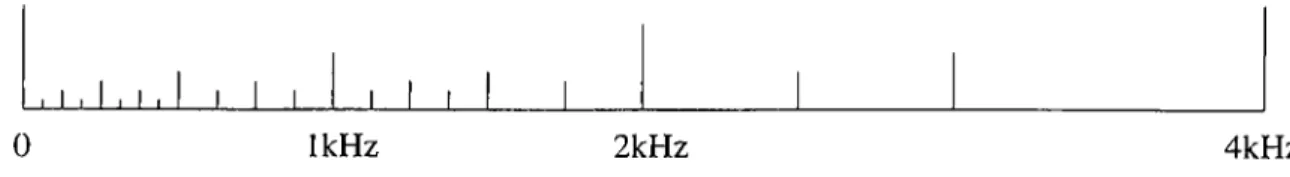
Figure 2.1. The sub-band frequency decomposition of the speech signal. The decomposition of the speech signal into sub-band signals is described in detail in [12]. In this thesis, the speech signal, s{n), is decomposed into L — 21 sub-signals, each of which is associated with,one of the bands in the frequency domain. The frequency content of the sub-signals are shown in Figure 2.1. The sub-band decomposition is almost the same as mel-scale. In other words, more emphasis is given to the .low frequencies compared to the high frequencies. For each sub-signal, the average iP-energy e; is computed as follows:

1 I

= T ^ ~ / = 1, 2, . . . , T

n = l

(2.3)

where Ti is the number of samples in the sub-band.

Log compression and Discrete Cosine Transformation (DCT) are applied to get TEO based cepstrum coefficients as follows:

TC{k) = ^ lo g (e /)c o s Â: = l , 2 ,...,1 2 (2.4)

where TC[k) is the TEO based cepstrum coefficient. The first 12 TEO based cepstrum coefficients form the first part of the feature parameters set. From the application of first-order differentials another 12 coefficients are ob tained. As a result, a 24-element feature vector consisting of TC{k) and dif ferentials is extracted from each frame of the speech signal. These vectors are also called observation vectors in speech recognition terminology.

(19)

2.2 E nd P oin t D e te c tio n

Locating the endpoints of a discrete utterance is an important problem in iso lated word speech recognition systems. A robust endpoint detection algorithm significantly improves the recognition rate of the overall systems.

The problem of detecting endpoints would seem to be relatively trivial, but in fact, it has been found to be very difficult in practice [2]. Usually the failure in endpoint detection is caused by: weak fricatives (/f/, /h /) or voiced fricatives that become unvoiced at the end of a word like in the Turkish word “yoz”, weak plosives at either end (/p /, / t / , /k /), and nasals at the end like in the Turkish word “dam”.

The wavelet analysis associated with a' sub-band decomposition of the speech signal is used in the endpoint detection algorithm [11]. Consider the decomposition of speech into L sub-signals as discussed in Section 2.1. The energy parameter Ef^ is defined for speech frame and sub-band as follows:

E t = ^ E 3?(n),

n = l

I — 1 , . . . , L (2.5)

where Ti is the number of samples in the sub-band. T; is smaller than the number of samples in the speech frame, if multirate processing is employed during sub-band decomposition. The distance measure Dk is then defined as

Dk = 10 log _t _E

/=1

(2.6)

where /i; and cr; are the mean and variance of the background noise at the sub-band, respectively. The speech free segments are used in the computation of /i; and (7; as follows:

(2.7)

(20)

— 7p — fiiY, k=l

/ = 1, 2, . . .,X.

(

2

.

8

)

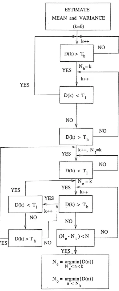
Figure 2.2 shows the flowchart of the endpoint detection algorithm. In this flowchart, T(,, Ti, and Th represent the beginning threshold, the lower threshold, and the higher threshold values, respectively. The lower and higher threshold values are defined in terms of the beginning threshold value as follows:

and

Th = - T b .

(2.9)

(2.10)

In Figure 2.2, Nb and Ng are the indices of the beginning and ending frame of a word in a discrete utterance, respectively, Nf is the maximum number of frames that the distance measure Dk stays below the beginning threshold

Tb-The algorithm scans the speech signal frame by frame and it marks the frame as Nb at which the thi’eshold value Tb is first exceeded unless the distance measure Dk falls below the threshold value Ti before exceeding the threshold value Th· After labeling a frame as Nb, the ending frame Ng is determined when the distance measure Dk falls below the threshold value Tb for longer than N f frames.

The threshold value Tb can be predetermined by the help of the histogram of the distance measure Dk (Equation 2.6). The performance of this end-point detection algorithm is significantly influenced by the choice of Nf value. If

N f is large then the algorithm may (1) miss the silent region between two

consecutive words; these words are treated as one word, or (2) treat silent regions at the end of the utterances as speech regions. On the other hand, if

N f is small then the algorithm may treat the utterance of one word as multiple

words. To overcome these problems, another parameter, Nd, is introduced and

N f value is chosen as small as possible. After detecting end-points of a discrete

utterance, if the number of frames between the ending frame of a word and the beginning frame of the consecutive word is smaller than Nd then the end points are changed so that these consecutive words are treated as one word.

(21)

Therefore, the distance between two consecutive words must be larger than Nj, frames.

The algorithm given in Figure 2.2 can be used to determine the end-points of a discrete utterance both at the time of recording and at any time after the recording is finished.

(22)

(23)

C h ap ter 3

H id d en M arkov M o d el (H M M )

for S p eech R e c o g n itio n

The speech recognition problem can be considered as mapping the sequence of feature vectors to a word in the dictionary. Starting from the late 1960s, researchers focused on developing stochastic models for speech signals. The reason they used the probabilistic modeling was to address the problem of variability. Today, Hidden Markov Model (HMM) and Artificial Neural Net works (ANN) are the two main approaches used in speech recognition research. The HMM approach is adopted in this thesis. The use of HMM models for speech recognition applications began in 1970s [21].

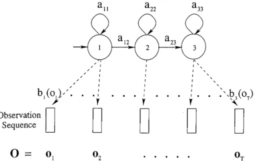
An HMM model is a finite state machine that changes state at every time unit as shown in Figure 3.1. At each discrete time instant t, transition occurs from state i to j , and the observation vector Ot is emitted with the probability density bj(ot). Moreover the transition from state i to j is also random and it occurs with the probability aij.

The underlying assumption of an HMM model in speech recognition prob lem is that a speech signal can be well characterized as a parametric random process, and the parameters of the stochastic process can be estimated in a precise and well-defined manner. An HMM model is considered as a generator of observation sequences (observation and feature sequences are used to refer

(24)

CHAPTER 3. HIDDEN MARKOV MODEL (HMM) FOR SPEECH RECOGNITION 12

a.

a .

a

₃₃

Observation Sequence

O = 0,

0 . • · · · · o .

Figure 3.1. A three-state left to right HMM model with the observation vectors each being generated by one state (state 1 I’epresents the start state).

the same thing in the rest of this thesis). In practice, only the observation sequence is known and the underlying state sequence is hidden. That is why this structure is called a Hidden Markov Model. This chapter introduces the theory of HMM models for speech recognition purpose.

3.1 E lem en ts o f an H M M

A complete specification of an HMM model requires specification of (1) two model parameters, N and M, (2) observation symbols, and (3) three sets of probability measures A, B, tt. The definitions of these parameters are as follows;

1. The parameter, N, is the-number of states in the HMM. The individual states are labeled as {1, 2, . . . , N}, and the state at time t is denoted as

qt-2. The parameter, M, is the number of distinct observation symbols per state. The observation symbols represent the physical output of the sys tem being modeled. The individual observation symbols are denoted

(25)

as V = { v i, V2, ... ,v m). Only in HMM models for discrete observa

tion symbols the parameter M is defined. HMM models for continuous observation sequences, as we have in this thesis, clearly do not have the parameter M, but have an observation set whose elements are continuous variables.

3. The matrix, A = {aij}, is the state transition probability distribution where aij is the transition probability from the state i to j, i.e..

“ij = P[ii+i = i I = >). I S S n (3.1)

If a state j can not be reached by a state i in a single transition, we have

Clij = 0 for all i , j.

4. Let O = ( o i,02, . . . ,oy) be the set of observation symbols. The matrix,

B = {f>j(Oi)}, is the observation symbol probability distribution in which

6j(o,) = P{o, I = i) , I < t < T (3.2)

defines the symbol distribution in state j , j = 1 , 2 , . . . , N. In speech recognition problem, observation symbols are feature parameter vectors. 5. The vector, tt = {TTi}, is the initial state distribution, in which

7T,( = P{qi = i), I < i < N. (3.3)

For convenience, we use the compact notation

\ = { A , B , n ) (3.4)

to indicate the complete parameter set of an HMM model. This parameter set defines a probability riieasure for a given observation sequence O, i.e., P ( 0 I A). VVe use HMM model to indicate the parameter set A and the associated probability measure interchangeably without ambiguity.

(26)

3.2 P ro b a b ility E valuation

One basic problem of HMM models is to calculate the probability of the ob servation sequence, O = (oj, 02, ... oy), given the HMM model A = (H, B, x). The trivial way of solving this problem is through enumerating every possible state sequence of length T (number of observations). Clearly, there are at most

such state sequences. For one such fixed-state sequence

q = {qici2 ..-qT)

(3.5)

where and qj are the initial and the final states respectively, the probability of the observation sequence O is

P (0 | q, A) = n i ’(o.

¿=1

(3.6)

In the equation above, the statistical independence of observations is assumed. In other words we have

P (0 I q,A) = 6„(0,).6„(02)...6„(07·).

(3.7)

Moreover, the probability of the state sequence q can be given as follows:

I “ ^91 ^7172 ^<72 73 · · · ^ ^ T - 1 qr-

(3.8)

Then the probability that O ^nd q occur simultaneously is simply the product of the two terms above, that is.

(27)

The probability of the observation sequence O given the model is obtained by summing the Equation 3.9 over all possible state sequences q, which is

P(0|A ) = X : />(0|q,A)P(q|A)

<7li92v.<7T

(02) . . . ^^qx^iq'T^q'T (o t). (3.10)

The interpretation of the Equation 3.10 is the following: At time i = 1 we are in state <71 with probability tt^j , and gene.rate the symbol Oi with probability

binioi). The clock changes from time t to time t + 1 and we make transition

from state to state q2 with probability and generate the symbol 02

with probability 6,2(02)· This computation continues until we make the last transition, at time T, from state qr-i to qr and generate the output symbol Ot

-It is clear that the calculation of P { 0 | Л) by using its direct definition (Equation 3.10) involves on the order of 2 T calculations. This computa tional complexity is infeasible even for small values of N' and T. For instance, for N = 5 and T = 100, there are 2 · 100-5^°° ~ 10'^ computations. Therefore, more efficient algorithms are needed.

The backward procedure and forward procedure are recursive methods of performing this calculation [1]. The crucial point of these algorithms is that each of them allows the calculation of the probability of a given state at a given time.

(28)

3.2.1 T h e Forward P ro ced u re

Consider the forward variable at{i) defined as

at{i) = P ( o i02 ...Ot,qt = i | A) (3.11)

that is, as the probability of the partial observation sequence, O1O2 .. - Of, and state i at time i, given the model A. We can solve Equation 3.11 for atii) inductively as follows: 1. Initialization 2. Induction o:i+i(i) = 3. Term ination ai(i) = 7r,-6,(oi), 1 < i < N. ■ N Y^at{i)aij i = l b j { o t + i ) , l < j < N N P ( 0 \ \ ) = Y ^ a T { i ) . i = l (3.12) (3.13) (3.14)

As can be seen from this iterative solution, the computation of P { 0 | A) requires on the order of N'^T calculations, rather than 2 T as required by the direct calculation in Equation 3.10.

3.2.2 T h e Backw ard P ro ced u re

In a similar manner, the backward variable A(f) can be defined as

/3t{i) = P(oi+iOi+2... orl^i = i, A) (3.15)

that is, as the probability of the partial observation sequence from i + 1 to the end, given state i at time t and the model A. Again we can solve for /?i(f) inductively, as follows:

(29)

CHAPTER 3. HIDDEN MARKOV MODEL (HMM) FOR SPEECH RECOGNITION 17 1. Initialization ^T{i) = 1, I < i < N. 2. Induction N K i < N. (.3.16) (3.17)

Again the computation of /3t{i) requires on the order of N'^T calculations like the forward procedure.

Both the backward procedure and forward procedure are used in “optimal” state sequence computation and parameter estimation algorithm in Section 3.3 and Section 3.4, respectively.

3.3 T h e “O p tim al” S ta te Sequence

An important problem in HMM model formulation is the estimation of the optimal state sequences. There are several ways to find the optimal state sequence associated with the given observation sequence. Various optimality ci'iteria can be defined.

Our optimality criterion is based on finding the state sequence which max imizes P (q I 0,A).· It is equivalent to maximizing F ( q , 0 | A) due to Bayes’ rule [9].

The solution is given by the Viterbi algorithm which is essentially a dy namic programming method [23]. Consider the Viterbi variable ¿((¿) defined as follows:

St(t) = max P(qiq2 ---(/i-i,qt = h 0i02. . . 0tlA) (3.18) 91,92.—i9t-l

where q = is the best state sequence for the given observation se quence O = (01O2 ... 02'). In other words, ¿¿(f) is the highest probability along

(30)

a single path, at time t, which accounts for the first t observations and ends in state i. The recursive version of 6t{i) can be written as

= m^x6t{i)aij bj{ot+i). (3.19)

The recursive procedure to find the single best state sequence is as follows;

1. In itia liz a tio n

<5i(0 = TTibi{oi), 1 < f < yV ^i(i) = 0

(3.20) (3.21)

where tpt(j) is used to keep track of the arguments that maximize the Equa tion 3.23 for each t and j.

2. R ecu rsio n Mj) = max [<5(_i(f)ap]6j(oi), ^ ^ M ) 3. T erm in a tio n r w i 1 2 < ( < r , a rg m a x (i,_ .(i)ai,l, (3.23) = max (3.24) = arg max (3.25)

where P* and the ql are the maximum likelihood of observing O in the model A and the state at time t in the final state seciuence which results in the prob ability P*, respectively.

4 . P a th (s ta te sequence) b ack track in g

q; = ^t+i(ir+i), i = P - 1, P - 2 , . . . , 1. (3.26)

As can be seen from the procedure above, Viterbi algorithm is similar to the forward procedure (Equations 3.12-3.14) except for the backtracking step.

(31)

TRe clifFerence is that, the summing step in the forward procedure (Equa tion 3.13) is changed with the maximization criterion (Ecpation 3.22) in the Viterbi algorithm.

The model parameters in Ecjuations 3.21—3.26 are very small values. The multiplications in the algorithm result in further smaller values. After a few iteration of the Viterbi algorithm, the result of these computations become 0 because of the limited representation (32-64 bit) for the floating numbers in computers. The Viterbi algorithm can be implemented without the need for any multiplication by taking the logarithms of the model parameters as follows:

0. Preprocessing Vi = log(vi), 1 < i < N bi{ot) = log(6i(oi)), 1 < i < N, 1 < t < T a,ij = log(a,j), l < i , j < N 1. Initialization (3.27) (3.28) (3.29) ¿i(i) = log(Si(i)) 2. Recursion Mj) = Vi + h{oi), 1 < i < V’i (0 = 0) 1 < i < = log(iiO)) (3.30) (3.31) max K i < N 2 < t < T , l < j < N . (3.32) M i ) = 3. Term ination arg max ° K i < N ^i-i(*) + dj· 2 < i < T, 1 < i < A^·

p · = maxi<i<,v [ir i·)] = arg maxi<K/v [¿r(0

(3.33)

(3.34) (3..3.5)

(32)

At P a th (s ta te sequence) b a ck trac k in g

(3.36)

This alternative implementation of the Viterbi algorithm requires on the or der of N^ T additions. The cost of preprocessing is negligible as it is performed once and saved.

3.4 P aram eter E stim a tio n

Parameter estimation is computationally the most difficult problem in HMM models. The model parameters P , and A are estimated to satisfy an op timization criterion. Our optimization criterion is based on maximizing

P [ 0 I A) where O represents the training observations. In order to do that, the

Baum-Welch method also known as expectation-maximization (EM) method is used [14].

Before going any further, the form of the observation symbol probability distribution, B = { b j { k ) } , needs to be made explicit. One can characterize ob

servations as discrete symbols chosen from a finite alphabet and use a discrete probability density within each state of the model. On the other hand, fea ture parameters extracted from the speech signals can take continuous values. Therefore continuous observation densities are used to model feature parame ters directly.

The output distributions are represented by Gaussian Mixture Densities. That is.

M

bj{ot) = Y^'cjkJ\i{ot,i.ijk,Ujk), I < j < N

k=l

(3.37)

where Ot is the observation vector being modeled, M is the number of mixture

values used for each state (in this thesis three mixture values { M = 3) are used

for each state), J\ f represents a Gaussian probability density function (pdf),

(33)

CHAPTER 3. HIDDEN MARKOV MODEL (HMM) FOR SPEECH RECOGNITION 21 M 'y / 1) ^jk ^ 0 ¿=1 1 < i < N, 1 < k < M (3.38)

The Gaussian pdf A/ has a mean vector fijk and covariance matrix Ujx. for the mixture component in state j , that is,

V w iu T

(3.39)

whei'e n is the dimensionality of the observation vector Ot. In our case n is 24, as 24 feature parameters are extracted from each frame of the speech signal as discussed in Section 2.1. Suppose that an HMM model contains just one state j and one mixture value k is used for this state. Then the parameter estimation would be easy. The maximum likelihood estimates of ¡Xjf; and Uj/,. would be simple averages as follows:

k'jk — rp <=1 (3.40) and _ 1 ~^jk — 7A ~ ~ k'jk') · t=l (3.41)

where T is the number of observations. In practice, HMM models contain more than one state; each of which has more than one mixture component. Moreover, for a given model and observation sequence, there are no direct assignments of observation vectors to the individual states, as the underlying state sequence is not knownr'However, Equations 3.40 and 3.41 can be used if some approximate assignments of observation vectors to the states could be done. Section 5.1.1 introduces the techniques used in the initial assignment of the observation vectors to the states of an HMM model.

We now define the variable ^t (hj ) [14] to help us in the parameter estima tion algorithm. The variable is the probability of being in state i at

(34)

tifne t, and state j at time t + 1, given the model A and observation sequence O, that is

itihj) = P{qt = ¿,9t+i =i|0,A). (3.42)

The variable can be re-written by using the definitions of the forward and backward variables (Sections 3.2.1 and 3.2.2) as follows:

U h i ) = Pjqt = hqt+i = i , O I A) P ( 0 I A) at{i)cUjbj{ot+iy/3t+i{j) P { 0 I A) atii)aijbj{oi+i)/3t+i{j) (3.43)

A posteriori variable 7<(i) [14] is defined for making the parameter estima tion algorithm tractable as follows:

7i(f) = P{qt = i I 0,A ) (3.44)

that is, as the probability of being in state i at time i, given the observation sequence O, and the model A. Then we can express as

7t{i) = P{qt = i \ 0 , X ) P{0,q t = i\X) P { 0 I A) P{0,qt = i\X) E g , F(0 , g , = i l X y (3.45)

The equation above can be re-written by the help of forward and backward variables as follows:

(35)

7t(i) = (3.46)

We can relate Ttii) to by summing over j , that is,

N

lt{i) =

i = l

(3.47)

The summation of 7i(2) over the time index t can be interpreted as the expected number of times that state i is visited. Similarly, summation of over t can be interpreted as the expected number of transitions from state i to j. That is.

T - l

7<(*) = expected number of transitions from state i (3.48) i = l

T - l

— expected number of transitions from state i to j (3.49)

i = l

If the current model is defined as A = {A, B, tt) then a set of reasonable

re-estimation formulas for the parameters of the model can be defined as in Equations 3.50—3.52.

Gij

expected number of times in state i at time i = 1 (3.50) expected number of transitions from state i to j

expected number of transitions from state i

M

h i^ t) = l < j < N k=l

(3.51)

(3.52)

In Equation 3.52, the formulas for the re-estimation of the coefficients

(36)

CHAPTER 3. HIDDEN MARKOV MODEL (HMM) FOR SPEECH RECOGNITION 24 E C l , U , k ) (3.53) E L E " i 7 < 0 . i · ) J^jk = E te i 7i(i. k)o, (3.54) iJjk = TJ=i l i( h - f t i ) ' (3.55) E Li7 . 0 , ^

where 7t(i, k) is the probability of being in state j at time t with the mixture component accounting for Oj. That is,

7 i ( i > =

^ j k · ^ l ^ j k } Uj/j)

a .(j w o n _Ylm=l Ujm).

(3.56)

At the end of these computations, a re-estimated model A — (A, 5 ,7t) is

obtained and either

• A = A, that is P { 0 \ A) = P { 0 \ A), or,

• model A is more likely than model A, that is P ( 0 | A) > P { 0 \ A) [1].

In this way, we can iteratively use A in place of A and repeat the re estimation calculations to improve the probability of O being observed from the model until some limiting point is reached.

In this thesis, triphones (Section 4.2) are used as the smallest unit for speech recognition. Each triphone is represented by a three-state left to right HMM model as illustrated in FigureArl. The algorithms described in this chapter are used on the HMM models of the triphones both in the training and recognition stage.

(37)

C h a p ter 4

T h e L an gu age M o d el

Designing the word model and the dictionary model is a challenging problem in speech recognition systems. They must be made in a way that allows for fast and accurate search algorithms. Moreover, it is a good idea to construct these models according to the needs of the language.

In this thesis, a Turkish corpus is used for gathering statistical information such as the most frequently used words/triphones, minimum set of triphones which covers most of the words in the corpus, etc. This corpus is constructed by collecting newspaper text on different subjects from the Internet, and it contains about 4.2 million words of which about 300000 are unique.

Section 4.1 gives a general overview of the Turkish language from the point of view of speech recognition problem. Next, the word model is introduced in Section 4.2. Finally, Section 4.3 introduces the dictionary model adopted in this thesis.

4.1 Turkish L anguage

This section examines the Turkish language from the point of view of speech recognition problem.

(38)

CHAPTER 4. THE LANGUAGE MODEL 26

Turkish is an agglutinative language. In agglutinative languages, bound morphemes are concatenated to a free morpheme. Each morpheme usually conveys one piece of morphological information such as tense, case, agreement, etc. The morphological structure of Turkish words has adverse impact both on recognition rate and system response time.

Let us examine the following two cases to understand the adverse impact on the recognition rate.

case 1: same stem, different suffixes

ev + (i)m ev + (i)n

In the first case, we have the same Turkish stem “ev” but different suffixes. The inflectional suffixes m and n are frequently used suffixes in Turkish but, unfortunately, their pronunciations are similar. Although the words “evim” and “evin” are different their pronunciations are very similar.

case 2: different stems, same sequence of suffixes

ev + lerinizdekilerden i§ + lerinizdekilerden

In this case, we have different Turkish stems namely “ev” and “i§” but the same sequence of suffixes. The pronunciation of the suffix part are the same in both words. Since the suffix part is about 90% of each word, the pronunciation of the words “evlerinizdekilerden” and “i§lerinizdekilerden” are very similar. Our solution to this problem is discussed in Section 5.2.2.

In Turkish, one can generate a large number of words which have the same stem but different suffixes. Therefore, even for a single stem the dictionary can contain quite large number of words with different suffixes. Increases in the size of the dictionary result in increases in the system response time.

(39)

4.2 W ord M o d el

Many HMM-basecl small vocabulary or even medium vocabulary speech recog nition systems assign fixed model topology to each of the words. That is, each HMM model in the system has the same number of states. In such systems, the smallest unit for recognition is the words themselves. It is impossible to use any part of the trained model of a word for the training or the recognition of different words. Such systems recognize only the words that are trained. Fixed-topology word models are not reasonable for large vocabulary speech recognition systems.

Many modern large vocabulary speech recognition systems use phonemes as the smallest unit for speech recognition. Usually one-state HMM models are used to model the phonemes of the language. In such strategies, the model of a word is obtained by cascading the models of the phonemes which make up the word.

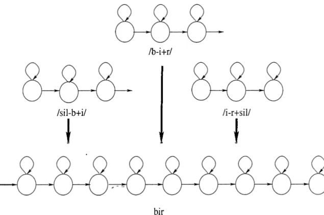
Turkish phonemes sound differently according to the phonetic context in which they appear. Neighboring phonemes aflfect the pronunciation of a phoneme significantly. Therefore modeling a phoneme with its phonetic context should give better results than modeling it individually. A good way of achieving this is to model each phoneme in the context of its left and right neighboring phoneme. This is known as the triphone model. The word “bir”, for instance, is represented by the following triphones

/sil-h + i/ /h-i+ r/ /i-v+ sill

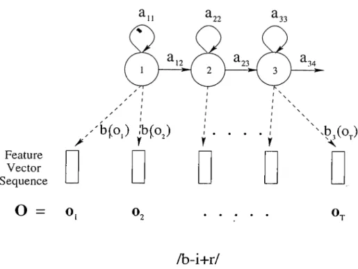
where sil stands for silent regions. Each phoneme in the word “bir” , namely / b /, / i/ , and / r / , is represented by a triphone. For example, the triphone /b -i-fr/ is used to model the phoneme / i / which has the phoneme / b / and phoneme / r / as the left and right neighboring phoneme, respectively. Using triphone models lead to a good phonetic discrimination [10].

Each triphone is represented by an HMM model A = (A, B , ir). This model has three emitting states and a simple left-right topology [1] as illustrated in

(40)

CHAPTER 4. THE LANGUAGE MODEL ₂₈ Feature Vector Sequence

O = o,

o . o .

/b -i+ r/

Figure 4.1. Example HMM model for the triphone /b -i+ r/.

Figure 4.1. As can be seen from the figure, the HMM model has the proj^erty that, as time increases, the state index either increases by one or stays the same. This fundamental property of the topology is expressed mathematically as follows:

a.ij = 0, where j < i, h j < N

i > j + l, i J < N (4.1)

The model states proceed from left to right. This topology is convenient to model the speech signal whose properties change over time in a successive manner. W ith this topology we have two special cases:

• Triphones which have / s i l/ at the leftmost position. They represent the beginning of words. The leftmost state in the HMM model of such triphones is interpreted as the start state in the HMM model of the words which begin with these triphones.

• Triphones which have ¡ s il/ at the rightmost position. They represent the ending of words. The last state in the HMM model of such a triphone

(41)

has another state transition constraint, a;vN = 1, in addition to the one in Equation 4.1 as ?he state sequence must end in state N .

For each state, a three-mixture (M = 3) Gaussian density is used as de scribed in Section 3.4. The memory requirement of an HMM model for a triphone is the sum of memory space needed for (1) mixture values:

A’ · {M · (n · S-D)) = 3 · (3 · (24 · 8)) = 1728 where N and M is the number of mixture values used for a state and the number of states in the model, re spectively, n is the dimensionality of feature vectors, and S-D is the memory space needed to store a double value in bytes, and (2) transition probabilities

N ■ (lY-T ■ S-D ) = 3 · (2 ■ 8) = 48 where N -T is the number of transitions from a state. That is, 1776 bytes are needed to store an HMM model for a triphone.

The model of a word is obtained by cascading the models of the triphones which make up the word. Figure 4.2 illustrates the process of constructing the HMM model for the word “bir”.

/b-i+r/

/sil-b+i/

I

bir

Figure 4.2. Example HMM model for the Turkish word “bir”.

We have a fixed model topology assigned to each triphone (Figure 4.1). On the other hand, the size of the word model depends on the number of triphones

(42)

in the word. Each word has its own HMM model which may have different number of states.

In the training stage (Section 5.1), first, the HMM model for a training word is constructed and trained. Next, the HMM models for the triphones which make up the word are extracted and stored individually. In the recognition stage (Section 5.2), we have the reverse operation, the HMM models for the triphones of a word are concatenated to construct the HMM model A of the word. This model is then used with the given observation sequence О to find

P { 0 I A). L e v e l 1: L e v e l 2; L e v e l 3: L e v e l 4: L e v e l 5: / s i l - a + t /

I

/ s i L b + i /

İnil I

/ а - t + s i l / — ► / a - t + І / ' 4

Л-

1

+sil/

F

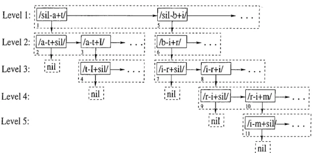
i / b - i + г / 11 '6 1 i / і - r + s i l / / І - Г + І / i7 i n i l : in il: _{/ г - i + s i l / — ► / г - i + m /} 10 ■nil ' I___I / i m + s i l f -i n -i l ■

Figure 4.3. Example dictionary which contains the Turkish words “a t” , “ati” , “bir” , “biri”, and “birim”. Nodeboxes and nodes are represented by dashed-rectangles and solid-rectangles, respectively.

4.3 T h e D ictio n a ry M o d el

The dictionary of a speech recognition system contains the words that can be recognized by the system. The design and implementation of the dictionary for Turkish is one of the challenging problems that was faced. The design of the dictionary must adhere to certain requirements:

(43)

• Turkish morphological structure must be taken into consideration in the design of the dictionary.

• The memory recjuirements must be as small as possible.

To meet the requirements above the dictionary model employed in this thesis is based on trie structure [24] as illustrated in Figure 4.3. A new ter minology, nodebox, is introduced here to make the algorithms defined on the trie tractable. A nodebox in the trie either contains nil corresponding to the termination nodebox, or it contains a linked-list of nodes each of which con tains a triphone and a pointer to a subtrie. It should be noted that a subtrie is, in fact, a nodebox with all the descendants. The trie is constructed with standard algorithms [24].

Figure 4.3 gives an example dictionary which has the Turkish words “a t” , “ati” , “bir”, “biri”, and “birim” . For instance, if we follow the nodes 1 and 2, we have the Turkish word “at” . It is understood that there is a valid Tiu’kish word because each word must have silent regions both at the beginning and at the end. If we follow the nodes 1,3, and 4, we have the word “a ti” which is the accusative form of “a t”.

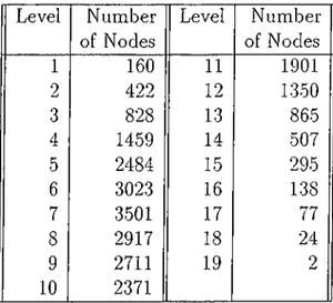
Table 4.1. The number of nodes at each level of the trie. Level Number of Nodes Level Number of Nodes 1 160 11 1901 2 422 12 1350 3 828 13 865 4 1459 14 507 5 2484 15 295 6 3023 16 138 7 3501 17 77 8 2917 18 24 9 2711 19 2 10 2371

All the triphones in the trie must be trained in the training stage. It is not possible to recognize a word containing a triphone which is not trained.

(44)

Though in the future this may be improved by allowing a self-correcting search algorithm such as the error-tolerant finite state recognition algorithm [25].

The words which are covered by the trained triphone models are chosen from the Turkish corpus and inserted into the dictionary. In this thesis, the depth of the trie is 19. Table 4.1 shows the number of nodes at each level of the trie. This table is included here in order to give a general idea about the search space.

This dictionary structure saves space because of the characteristic of trie data structure and Turkish morphological structure. Moreover it allows for fast and accurate search algorithms as discussed in Section 5.2.2.

(45)

C h a p ter 5

T h e T raining and R e c o g n itio n

S ta g e s

A spoken word can be represented by a sequence of observation vectors O, defined as O = Oi , Oi , . . . , ox where Oj is the observation vector and T is the number of observation vectors for a single word utterance. Then the problem of isolated word recognition can be defined as

w* = argmaxP(ri;,· | O) (5.1)

where iVi is the word in the dictionary and w* is the desired word. By using Bayes’ rule, P{wi | O) can be expressed as follows:

P { w i I O) =

P { 0 I Wi)P{wi)

P(0) (5.2)

Prior probabilities P{tUi) are taken to be equal to each other for all to,· in this thesis. Therefore the most probable spoken word depends only on the likelihood P ( 0 | roi). It is not feasible, for a given observation sequence O, to directly estimate the joint probability T (oi, 02, . . . , Ox | W{) for each word lUi as discussed in Section 3.4. HMM models introduced in Chapter 3 are used in this thesis so that computing P { 0 \ Wi) is replaced by estimating the HMM

(46)

CHAPTER 5. THE TRAINING AND RECOGNITION STAGES 34

model parameters of the word wi.

Triphones are used as the smallest unit for training and recognition of the words. The training of these models and their usages in recognition stage will be introduced in Section 5.1 and Section 5.2, I'espectively.

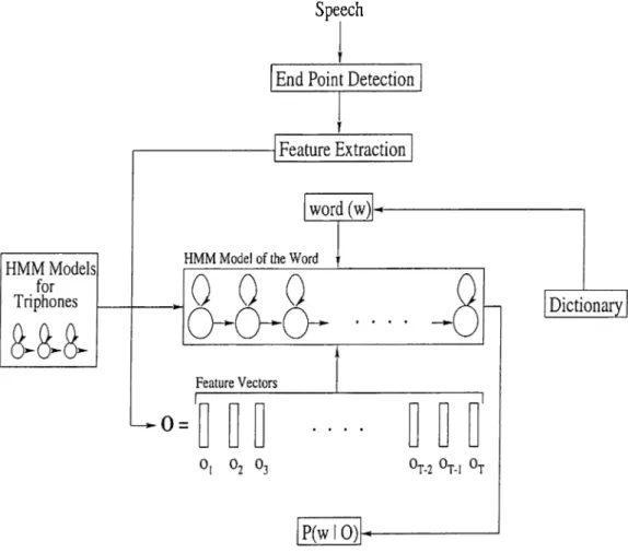
The general architecture of the speech recognition system developed in this thesis is given in Figure 5.1. As can be seen from the figure, after feature extraction step, the trained HMM models of the triphones are used to con struct the HMM model of a word w supplied by the dictionary. The Viterbi algorithm is then applied to the HMM model with the feature vectors to get the probability P{w \ O). Later, in Section 5.2.2, this architecture is powered with a search strategy for a word in the dictionary.

Speech

(47)

5.1 T h e T raining P ro cess

Several training algorithms for HMM models were introduced in [20], [3], [6], and [8]. The training algorithm used in this thesis has 4 steps for a given word:

1. Construct the HMM model topology of the word.

2. Guess initial set of model parameters for the HMM model. 3. Improve the HMM model.

4. Save individual HMM models for each triphone in the word separately.

In this way, the words that are not trained, can be recognized. For instance, once the word “okul” is trained, we have four HMM models for the triphones

/sil-o + k /, /o -k + u /, /k-u+1/, and /u-l+ sil/. In the recognition stage, we

can use the models for the triphones /k-u+1/ and /u -l+ sH / to construct the HMM model of the word “kul” (triphones for “kul” is /sf/-k + u /, /k-u+1/, and /u -l+ sil/) assuming that the triphone model for /sil-k + u / is also trained. Therefore, the word “kul” does not need to be trained.

In the algorithm above and throughout this section, it is assumed that an HMM model is trained by using single utterance of a word. However, in order to get good HMM models three utterances of a word are used. The use of multiple observation sequences adds no additional complexity to the algorithm above. Step 3 is simply repeated for each distinct training sequence.

The Turkish corpus is used to determine the words that will be trained. One of the strategies to choose the words for training is to select the minimum number of words whose triphones cover most of the words in the corpus. This strategy favors the long words in the corpus. Simulation results show that using triphone models obtained by training long words has negative effects on recognition rate because it is usually difficult to pronounce too long words. Therefore a constraint on the length of the words is also used in the selection of the words. This strategy allows us to find about 1200 words (of maximum ten letters long) whose triphones cover 90% percent of the words in the corpus. That is, if we train about 1200 words, we can theoretically include 90% percent of the words in the corpus.

(48)

In order to increase the recognition rates of the most frequently used words and have a manageable dictionary size, a second strategy is introduced to select the words. This strategy simply chooses the most frequently used words in the corpus for training.

For the rest of this section, assume that a training word has T frames in the speech signal, N ST P triphones from which N -V of them contains a vowel or semi vowel in the middle, N states, and the HMM model \{ A , B .it).

5.1.1 In itia l G uess o f th e H M M M o d el P a ra m eter s

Every training algorithm must start with an initial guess. This section in troduces the strategy to guess initial parameters for the HMM model A = (A ,5 ,7t). The training word may have triphones which may already

have been trained. If that is the case, these trained models are used as the initial guess, otherwise, the model parameter A, B, and tt are initialy guessed as follows:

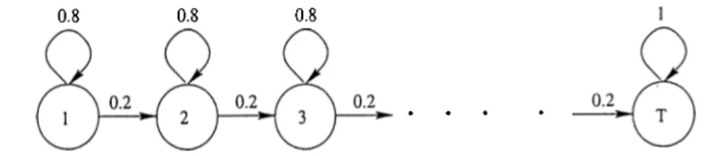
I n itia l G uess of th e s ta te tra n s itio n p ro b a b ility d is trib u tio n , A: The initial guess of the state transition probability distribution is given in Figure 5.2.

0.8 0.8 0.8

Figure 5.2. Initial estimate of the state transition probability distribution, A. The triphones which have / s i l/ at the rightmost phoneme position have only one state transition for the rightmost state. This transition goes from the rightmost state to itself because there is no other state on the right. Since the sum of the outgoing transition probabilities for a state must be 1, the proba bility of taking this transition is 1.

(49)

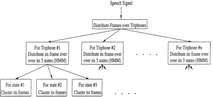
In itia l G uess of th e o b serv atio n sym bol p ro b a b ility d is trib u tio n , B: As described in Section 3.4, in order to apply parameter estimation formulas (Equations 3.50—3.56), some approximate assignments of observation vectors to the individual states must be done. In this thesis, feature vectors extracted from the speech signal are distributed on the states of an HMM uniformly. In fact, more feature vectors are assigned to the states corresponding to the vow els or semi-vowels than those corresponding to the plosive consonants or the weak fricatives. Triphones that have vowels or semi vowels in the middle get 2 * yv_r/^/v_v vectors whereas the others get v f^^fure vectors.

After assigning the feature vectors on triphones, we distribute feature vec tors for a triphone over its three states such that, first one fifth of the feature vectors are assigned to the first state, next three fifths are assigned to the sec ond state, and the last one fifth are assigned to the third state. Although this distribution is static, later in the improvement of HMM models (Section 5.1.2), the Viterbi algorithm is used to modify this static distribution of the feature vectors on the states . Figure 5.3 illustrates the distribution of feature vectors on the states.

Speech Signal

Figure 5.3. Distribution of feature vectors on to the states.

As discussed in Section 3.4, continuous observation densities with three mixture values (M = 3) for each state are used in this thesis. K-means cluster ing algorithm [15] is used to cluster the feature vectors within each state j into

(50)

a set of M clusters (using a Euclidean distance measure), where each cluster represents one of the M mixtures of the bj{ot). These mixture values are used with the given observation sequence O and the Equation 3.37 to compute the observation symbol probability distribution, B , for each state.

Initial sta te distribution, tt:

The HMM model for a word has only one starting state. Therefore, we have TTi = 1 and 7T,· = 0 for all i where i = 2, 3, . . . , N .

At the end of these computations, we have the initial HMM model A = ( A , B , x ) for the training word.

5 .1 .2

Im p rovin g th e H M M M o d el

Improvement of the model A = (A, B, tt) means that the parameters of the

model have to be re-estimated to get an improved model A = (A, 5 , tt).

As Figure 5.4 illustrates, there are three main steps in the improvement of an HMM.

First, we find the optimum state sequence for the given model A = (A, B , tt)

and given observation sequence O by using Viterbi algorithm. Optimum state sequence determines which state emits which frames. Therefore we can consider the Viterbi algorithm as an another way of distributing feature vectors on the states of an HMM model such that F ( 0 | A) is maximized.

Second, for each state, K-means clustering algorithm are used to reestimate the clusters of its feature vectors according to the number of mixture used. The clusters may change since we change the distribution of the feature vectors on the states in the first step.

Finally, the Equations 3.50—3.55 are used to reestimate the parameters of the model A = (A, B ,7r) to get the new improved model A = (A, B ,tt). Note

that the parameter tt did not change because the new model should have also