Residual lifetime distribution and its applications

RESIDUAL LIFETIME DISTRIBUTION AND ITS APPLICATIONS I M. M. SIDDIQUI

Department of Statistics, Colorado State University, Colorado, U.S.A. and

M. ~ A ~ L A R

CEOR-Engr. Quad, Princeton University, Princeton, NJ 08544, U.S.A.

(Received for publication 29 December 1992)

Abstract- Let T be a continuous positive random variable representing the lifetime of an entity. This entity could he a human being, an animal or a plant~ or a component of a mechanical or e]ectricai system. For nonliving objects the lifetime is defined as the total amount of time for which the en- t i t y carries out its function satisfactorily. The concept of ag/n 9 involves the adverse effects of age such as increased probability of failure due to wear. In this paper, we consider certain characteristics of the residual lifetime distri- bution at age t, such as the mean~ median, and variance, as describing aging. G a m m a and Weibull families of distributions &re studied from this point of view. Explicit asymptotic expressions for the mean, variance and the per- centilea of corresponding residual lifetime distributions are found. Finally these families of distributions are fitted to four sets of actual data, two of which are entirely new. The results can be used in discriminating different shape parameters.

1

I n t r o d u c t i o n

In reliability theory, we&rout failures which are s symptom of aging, occupy an important place. Several criteria for the concept of ag/ng of a piece of equipment with s well defined survival time distribution is considered in Bryson and Siddiqul [1]. Additional criteria can also be found in Deshpande et. al. [2] In general, mean residual life (MRL) function provides s more descriptive measure of an aging process than the hazard function. They &re two of the functions which completely specify the distribution [3]. Let T represent the lifetime of an item and have a specified distribution function, t h e n the distribution of T - t given T > t is the residual lifetime distribution 1The work of the authors was carried out when the first author was a visiting professor and the second author was a graduate student at Bilkent University, Turkey during the academic year of 1990-1991.

212 M.M. SIDDIQUI and M. ~A(~LAR

at time t > 0. In this paper, residual lifetime distribution is discussed in terms of its mean, variance and percentiles as describing aging, and behavior of those quantities as t tends to infinity, for certain distributions. Lawless [4] provides a relationship between the asymptotic value of MILL and the pdf. Moreover, Calabria and Pulcini [5] provide a relationship between the asymptotic behaviors of MRL and the hazard rate. In our study of asymp- totic behavior of MRL, we have additionally found the order of convergence to the limits that were found in these studies.

Because of its simplicity, Exponential distribution is widely used. This distribution has memoriless property which is equivalent to no

ag~c~g

in relia- bility context. However there are situations where the property of no memory (equivalently no aging or wearout) does not agree with the physical realities, as is the case when T represents a service time or a repair time, or when failure is due to wearout. Weibul] and Gamma are two typical distributions which describe the lifetime of an aging piece of equipment when the cor- responding shape parameter is greater than 1. Hence,they are investigated from the point of view mentioned, in sections 2 and 3, respectively. Finally, in section 4, four sets of data are analyzed to apply the use of the properties of residual life distributions, such as the mean and the variance, for selecting one or more theoretical distributions which adequately fit the data.

Notation

T lifetime of an item

f(t)

pdf for lifetime

R(t) reliability function, R(t) = Pr{T > t}

fT-,(.)

pdf for residual lifetime, f T - t ( z ) = f ( z +

t)/R(t)

M(.) moment generating function

e(.) mean residual lifetime ~(.) variance of residual lifetime P(a) G a m m a function [6, 6.1] ~v pth percentile of residual lifetime

shape parameter scale parameter Z + set of positive integers

The pdf's of Gamma and WeibuLl Distributions ( f and g respectively) are given for 2 parameters, shape and scale, as follows:

2

R e s i d u a l

L i f e t i m e

f o r G a m m a

F a m i l y

o f

D i s t r i b u t i o n s

For the sake of simplicity, let us first consider G a m m a Distribution with integer shape parameter n. Then, the reliability function is

_f** .~"="-'e-"'~_~ _ "-"~ (~Ohe

-'~'~ ,

R(t)

and the density of the residual life time distribution is & _ , ( = ) = ~"(=

+ t),,.-,,,-~,c=+o

The density function simplifies to

f~-,C=) = ~'C= + 0 "-~,-~"

(n -

l~v _{~1" [--~k=O k!}

x----a (xq~

The moment generating function is

[** e"a"C= + t) "-1"-~= d=

M(s)

J0

/-ak=O k! which by integration by parts, is simplified as follows:

~ ( , ) = ( ~ ) .

E;:o ~ fc~;~,l,

~;:o ~ c~:?,

So the expectation of residual lifetime e(t):

• ~"~n--1 ( n - k ) A h - t t h

e( 0 = M,(,)l.=o = "k=o

~Z

The second moment:

M"Cs)l.=o = E~=°~ (--~i(--h+~)~'-','~

_YlI--] ~"~k=0 k! As a result the variance of residual lifetime v(Q:

(n-h)~ h-1

t h

~2

v(t) = L'~L--°a (,~-k)¢,~-,+a)x'-=,'._1

~# I

- (E~n--'-°It~--x xt.~_~

~2hl ,

(2)

~"~4,=o k! k~k=o k! /

The percentiles of the residual life distribution at age ~ can be found as follows. Since

P{T

- t > =IT > t) -- ("-~>'

~p, the p ~ percentile, is the solution of the following equation in z:

1 - n = P { T - t > = I T > ~ }

e-X=

x--,n-1 (=+t)~a '

=

z.,k=o

/~

~;'°

z ~

(3)

This equstion cannot be solved exactly for an arbitrary integer n. That is why the asymptotic behavior will be discussed in the next section.

214 M.M. SIDDIQUI and M. ~A~LAR

A s y m p t o t i c Behavior of Mean, Variance a n d P e r c e n t i l e s

of Residual Lifetime

L i f e t i m e d i s t r i b u t i o n w i t h i n t e g e r s h a p e p a r a m e t e r

For n = 1, the residual lifetime distribution is reduced to an exponential distribution, so e(t) = 1/A V t _> 0.

For n -- 2, from equation 1, e(t) = (~/~+t)l+~t -- ~(1+~)1 + ~'1 Then, at t--0,eCt) = 2/A and as t ~ oo e(t) = 1/A %

O(I/t).

For n E Z +, from equation 1,

e(t) = n/;~ + (n - 1)t/1! + (,~ - 2)At~12! + . . . -t- ;~"-~e-~/(,~ - 1)! 1 + ;~t/l! + ; ~ O / 2 ! + " . + ;~"-~t"-~/('~ - 1)! Then, at t = 0,,(t) = ,q,X and as t ~ oo ~(t) = 1/;~ + O ( l / t ) .

Similarly, for the variance starting with n = 1, 2 : For n = i, v(t) = I / A V t > 0.

For,~ = 2, from equation 2, at t = 0 ~(t) = 2/A ~ a n d as t -. oo ~(t) = 1/A 2 + O(1/t)

For n E Z + from equation 2, writing the smallest and highest orders of t

with their coei~cients in the summations:

(

~_~..I

+ . . . + (,,-17., (,-1?, J [(,~-1), 1, J ~(~) = (~t)1(~-1} 1 + ... + [(n_l)~I we obtain + . . . + 'U(~) 1-t- ... -I- ~ T h e n , a t t = 0 , , ( t ) = n/,X 2 a n d as t - , oo ,,(~) = Z/,X 2 + O ( 1 / 0 , because , ( t ) 1 ( n - 1) + - . - + ~ = O ( l l t ) for large t.

As stated in the previous section, the percentiles must also be studied for large t. For n = 1, {e = - log(1 -

p)/A.

Let us denote the pta percentile corresponding to the residual lifetime with shape parameter n as ~ ( n ) .

Then, for n -- 2 from equation 3,

e-~(,(~)[1 + (~,(2) + t)A]

l - p = 1 + A t

B y simplification, the following is found:

A,~,(2).

A~,(2) = log(1 + 1--~-~) -{- A(,(1) .

But, for large t, the denominator of the second term in the logarithmic func- tion also becomes large and the approximation log(1 + z) ~ z can be used.

So for large t,

1

~¢,(2)[1 - 1---~-~- ] ---- ~,(1) or

For arbitrary n, taking logarithm of both lides of equation 3,

-;~=+tog[l+~+.. " (;~(= + t))"-~ ;~t ' (;~t)"-~ '

l o g ( l - p ) •

+

~ - ~

] - l o g [ l + F + ' " - , - ~ , By simplification and by writing the smallest and the highest orders of t in the summations, we get

- 2 _ . . z . . . (,,_2)i 1 1 log[1 + ~ z " ~ " 12 , ~_ . >.,,-1,,,-==

Then, using the approximation log(1 + =) ~ z as we did for n = 2 for large t, we have

z + ,~='12 + . . . + ( ~ O " - ' z I ( , ~ - 2)!

=~-

1 ¥ Y F - ~ - : ¥ ~ ~ ) ~

+~,(1) .

But for large t, the last terms in the numerator and denominator respectively dominate, so that (,Xt)"-'=/(,', - 2)! + ,~,(1) = ~ (~,O"-V(,', - 1)! This gives n - - I " ~ ' ' I " , =[1 - - - ~ ] -- ¢ , ( ) or finally, n - 1 z = ~p(1)[1 +

T

+ O ( 1 / t 2 ) ] "

The last equation is written by the identity ~ = ~-~'=0 zh for sui~clently small z > 0. Now z stands for ~,(n), so for large t, ~,(n) = ~p(1) +

O(llt).

These axe interesting results, because this means that if an item whose lifetime distribution is defined by a G a m m a Distribution (with integer shape parameter) survives a long time, then it behaves asymptotically as if it has an exponential residual lifetlme distribution, i.e., it behaves as if it does not age any more. Moreover, for n E {I, 2 , . . . } it can be concluded that both e(t) and ~(t) are decreasing functions of t. And for large t,the order of decrease is o ( 1 / 0 .

G e n e r a l i z a t i o n t o r e a l s h a p e p a r a m e t e r

The mean residual lifetime in general is

e ( O = f,'=' = f ( = ) _{R ( O - , ~ . ( 4 )}

By writing the density and the reliability functions explicitly in 4 and by simplification, we get

e(t)

= ~® =Be-~,- dz

f ~ z~-ze-~

-- f..

216 M.M. SIDDIQUI and M. CA~LAR

ator, and calling the integral in the denominator I1, the result in terms of I1 only, is:

e(t) = I (/~ - 1)x, + ~ e -~' - ~tx~

Now, let lh = ~ zB-ke - ~ d~z and apply integration by parts several times: i ~ + (D-n'~-2le~tls - (#-nfD-2lfD-alte;Xt/4~%, e(0 = ~ + t#-~ + (/~ -

1)e~"x.,

Finally, for large t)

e(t) = ~ + o( ) = ~ + o( ) ,

as in the case of integer shape parameter.

The variance for the general case is studied in the same manner. It is explicitly:

.(t) = E { T ' I T > t} - E ' { T I T > ~}

I? ,'f(,)~ ($r-f(=)~)'

=

a(,)

a,(,)

Putting the expressions of a ( t ) a n d / ( z ) , a n d applying integration by parts several times, we get

1 M-*)M-3X~-a)~'+*eX' I4 -- a(~-2)f~-I)~MeA' -/'3

so that

1 O(t ~-~) 1 1

~(t) = ~ + o(t--'---5 = ~-~ + o(_)

Percentiles of the residual lifetime distribution can be obtained in the same way as the percentiles for integer shape parameter. L e t , < ~ / < n + 1. Then the real shape parameter version of 3 is

(/.

~B(, + O#-~e-~c'+')r(#)

d,)/(~"

~:-~e-~'r(~)

d,)

1 P

Putting u = z + t, and simplifying the righthand side, we obtain fffi~¢ u ~-1 • -'~u du

1

--p

=

ft.z~_,e_~,d z

By integration by parts several times, it is found that

(.+t)"-'.-~-+') + (#-x)(.+tf-',-'~.+') + . . . + (~-,)..~-.+,)r, (p-1)~e-,. -~, (~-x).J~-.+,)/, , + 42 + " " + ~,,-x where

I1 = ~:tu~-"e-X" du

Is = L °° u~-ne -~u du

Let's call the numerator of last equation as a and the denominator as b . Then taking the logarithm of both sides,

By rearranging the logarithm terms on the righthand side and writing the smallest and highest orders of ~ in the summations,

(/J-1~-:l~+"~'ffJ-1)...ffJ-"+D'x('÷')l~l~'-11

log(1 - p) = - ~ = + log[1 + ~-~lX+...+(IJ-1)...(lJ-,,+l),~'z2p,"-~ J

Because, for large t, the algebraic term inside the logarithm function in the last equation becomes small; we can use the approximation Iog(I -I- z) ~ z. As s result,

z ~ ' 1 (B_I~.~-~I~+...+(Ij_I)...(Ij_n+I~X(.+OILI~,,,-~ _{-- ~ ~-'/,~+...+(,e-1)...¢,6-,+1),"'.",/,~--'. + ,~p(1) .}

Moreover for large t, the highest orders of t are the dominating terms in both the numerator and the denominator, so that

,., 1 (,8- 1)=~'6-~/A + ~,(1) o r = _~

(,8-

1)z and finally z = [ l + + O(lltS)] ~,(1) V,8>O

So, all results pertaining to integer shape parameter case are also valid for real shape parameter. Moreover, these results suggest that, in model selection we have to study the MRL plots for relatively small t, in order to discriminate between different shape parameters of Gamma distribution, because for large t they all converge to 1/A and thus discrimination becomes difficult. W h a t is more, the results can be used in debugging or burn-ln processes. For example, some traxie off can be found in terms of the testing period; the MRL of the items decreases when they are debugged, but on the contrary the residual lifetime becomes more stable in terms of both its mean and the variance.

3

R e s i d u a l L i f e t i m e for W e i b u l l F a m i l y o f

D i s t r i b u t i o n s

The residual lifetime density is

f~_,(~) = ,e~"(=

+ t~-'.e-t~'('+')]"

e-(,~tp The moment generating function is

M(+) = f0" e"[~(® + O]"-"e-t~'C'+')~'~.e ,~

e _ ( , ~

by using the identity e" = ~ o ~ and by making a change of variable u =

[,~(=

+ t)],~i we

get

M ( a ) -- e - " ~'(,~/A~' f('~e~'u'q'ee-" du - ~:o J.Lt -t- l)

218 M.M. SIDDIQUI and M. CA~LAR

Let

r(.,=) = f"¢-'e-"

d~

.

Then the m o m e n t generating function is found as e - " ~ . . . . ~I"(i/#9 + 1 , ( A t ) a ) - Z . , L s / A ) : , ~ - - - M(a) e-(~O# i=o .L'(j, + 1)

and mean residual lifetime

is

e ( 0 = M'(*)l,=0 = r ( 1 ÷ 1/#9,

CAt)a)

_ ~: Ae_(;~#,

The second moment is

M"(s)l.=o = P - 2tr(1 + 11#9 , (At) a) Jr r(1 + 2/#9,(At)a)

Ae-(;~ty' A',e-(;~,y'

,

so the variance is found as

.(t) = r(l+2/#9,(At)a) r2(1+ 1/#9,(At)a)

A2e_(.,,,y, - A~e_.,(;~,y, (5) The pth percentile ~e is the solution of the following equation in z:

p = P { T - t < = I T > t} = g #gA[A(,V + t)]#-*e-[~('+')]' d~

- e_(~ty,

Evaluating the integral in the last expression by putting u = [A(9 + t)] ~, we

get

e-(XtY' _ e-l,~(-+t)F p = e( _,x,,),e , and finally ~ = t[1 log(1

-

P)]xl/J

_ t . (6)

(At)a

A s y m p t o t i c B e h a v i o r o f E x p e c t a t i o n , V a r i a n c e a n d P e r -

c e n t i l e s o f R e s i d u a l L i f e t i m e D i s t r i b u t i o n

At t = 0, e(t) = r(l+xl/~), which is the expected value of T. For t > 0,

e( 0 = r(1 + 1/#, CAt)a) _ t (7)

Ae_(X0p

and in open form, r ( 1 + 1//3, CAt)a) = f(~ty, u l m e - " du. By integration by parts, this can be reduced to

r 0 + 1/#9, (At)a) = Au-c~,~ + ~ 0 e -'~ ~

(8)

L e t / 1

= f ~

e - ~ ' d.z. I1 cannot be evaluated but an approximation for large t can be found. By integration by parts, it can be shown t h a t

e-( x'y' . / 9 - i e -¢~*y' # 9 ~ 1 1 - ~(-5-T?p] < I, _< #9(AO,,_ ~

Then, for large t,

e-(X0P

By putting this first in equation 8, then in equation 7, and by simplification, for large L, we obtain:

1

eCt) --/9,~(~t~s_1.[l +

O(llt~)]

This l~,t expression is valid for large t only, but it is much more practical for computation than equation 7.

So

0 f o r 3 > 1 tlimeCt)= oo foe 0 < ~ < 1

And for #8 -- 1, e(t) = 1/A.

The variance (in equation 5) can be studied in a similar fashion, then in open form,

r ( l

+ 2/~, (AL~

s) = ~:~

u21~e-~'du

i

By a change of variable u -- z ~ and by integration by parts, we have r(1 + 21/3 , (At~ s) = A't'e -(Aty) + 2 J ~ ze -~) (/z

(10)

Let/~ = J'~ ze -'# d~z. For large t, /2 can be approximated as

e-(~#'

/2 = ~ [ 1 + O(1/t~)] .

Cancellation occurs with r2(1 + 1/~, (At~ s) in which there is l,,which is also approximated as in equation 9. So, one more step is taken in approximation

for both/i and for/2. T h e results are as follows:

e-(~Os(~(At) p - ~ + 1)[1 +

O(1/t'/~)] ;

e-(~OSC/9(At~ s - ~ + 2)

/2 = 132(At)2~_ , [1 +

0(11t2#)]

.

Putting those expressions in equation 8 and equation 10 respectively) then

putting the results in equation 5, we obtain

~(At~LS(At~ -I-

2(~ - 1)] - (1 -~)211

A2tg,(At),s-2

+ O(llt2B)]

and o for ~ > I ~(~)

I

co /or

0<19<1

For ~ - 1, ~ ( t ) = I/A ~.

The asymptotic behavior of the percentiles can be studied in relation to equation 6 as foUows, using the fact that - log(1 - p) < (At) 2 for large t, by the binomial expansion formula,

1 l o g ( I - p ) . 1,1 1,1og2(1-p) 1.1 .-1 loga(1-p) .

~,=~[1 ~ 1!(~)~ ~ -

~ 2.-~(~F~ ~(~-1)(~-2) ~

+...j-~ ,

so that

t l o g ( 1 - P) i'" 1 _ 1,1o=gg(_1:.=p) 1 1)(~ -2)l°g)~-~(~t~=-~P)

220 M.M. SIDDIQUI and M. ~A~LAR

t log(1 - p)[1

= - 3 ( ~ t ) ~ + O ( 1 / ~ ) ] So

0 f o r 3 > i

lim~,=

oo for 0</~<i

The above result is valid for/~ ~ I. For ~ = I, the distribution is reduced to the exponential distribution which has been discussed in the previous section.

Having found the expressions for large t, for e(t), v(t), and ~ we can conclude that the greater the shape parameter the faster the convergence to 0 (when ~ > 1), and the same is valid for the variance and the percentiles of the residual lifetime. In other words, when the item's lifetime is explained by Weibull distribution, the aging process is much severe for larger shape parameters. Hence, this property can be considered in discrimination of dif- ferent shape parameters of Weibull distribution or in discrimination between different types of distributions.

4

D a t a A n a l y s i s a n d C o n c l u s i o n

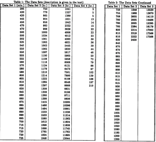
In this chapter, four different sets of data are studied for the purpose of applying the mean residual lifetime function as a criterion for aging. The first two sets are lifetimes of 75 Watt bulbs produced in two different Turkish factories; the third one is the lifetime of Kevlar 49/Epoxy Strands [7] (tested at 70% stress level), and the last one is the service time between failures of the air-conditioning equipment in Boeing 720 jet aircraft [8]. For this last set, the essential assumption is that after repair the equipment becomes as good as new. The first three sets of data are examples of items with decreasing mean residual life, i.e., the items are aging in time. Conversely, the last data set is an example of exponentially distributed time between failures (lifetimes, in a sense). The reason for selecting decreasing mean residual lifetime distributions is the greater importance of aging items in production environment than those with no aging, in terms of quality. The data are given in tables 1 and 2.

At this point it must be stated that data set 1 and data set 2 are ordered statistics taken from random samples, tested under 320 Volts and 286 Volts, respectively, voltages which are never encountered during normal usages of those bulbs. These high voltages are only for shortening the test period and observing all of the bulbs' lifetime, since under 220 Volts the lifetime of a bulb may be in years.

T h e natural e s t i m a t o r for the m e a n residual lifetime function is: $

= s - ' ,(tj - t) ,

j = l

where .g denotes t h e n u m b e r of survivors at t i m e t out of an initial population of size N , and {tj : j = 1 , . . . , S} is the set of d a t a points which are greater than t.

Since t h e first three d a t a sets show decreasing m e a n residual lifetime, G a m m a and Weibull distributions were fitted to them. Moreover t h e y reveal the presence of a truncation parameter, because the smallest value in t h e set is comparatively high. We fitted three p a r a m e t e r Weibull and O a m m a distributions. In estimation procedure, we e s t i m a t e d truncation p a r a m e t e r by the smallest d a t a point (let it be z l ) , t h e n transferred the d a t a to a new one by subtracting zl from each d a t a point. T h e n we fitted two p a r a m e t e r Weibull and G a m m a distributions to the transferred data set. We have used m o m e n t estimators.

Table 1: The DataSets (description m given in the text) Table 2 : T h e D a t a SetaContinued Data Set 1 (min.) Data Set 2 (hr.) Data Set 3 (hr.) Data Set 4 (hr.) Data Set 1 Data Set 2 Data Set 3

295 750 1051 3 750 1946 13520 420 778 1337 5 755 1968 13670 420 865 1389 5 768 2005 14110 445 904 1921 13 780 2005 14496 450 956 1942 14 780 2005 15395 470 983 2322 15 785 2264 16179 470 988 3629 22 800 2314 17092 500 1000 4006 22 810 2319 17568 500 1034 4012 23 810 2332 17568 502 1061 4063 30 830 2458 525 1063 4921 36 840 540 1063 5445 30 870 550 1065 5620 44 870 550 1097 5817 46 870 555 1100 5905 50 885 555 1108 5956 72 885 560 1116 6068 79 890 570 1124 6121 88 900 580 1179 6473 97 909 580 1210 7501 102 910 600 1214 7886 139 915 605 1222 8106 188 915 610 1285 8546 197 915 630 1297 8666 210 930 630 1308 8831 950 645 1308 9106 960 660 1380 9711 960 660 1399 9806 960 875 1415 10205 980 685 1466 10396 990 690 1494 10861 990 890 1533 11026 1005 690 1533 11214 1005 695 1580 11362 1020 700 1612 11604 1050 715 1698 11608 1050 715 1698 11745 1080 720 1765 11762 1185 720 1824 11895 1200 725 1940 12044 1200

222 M.M. S|DDIQU] and M. (~A(~LAR

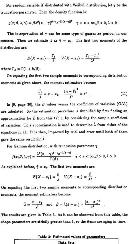
For r a n d o m variable X distributed with Weibull distribution, let 3' be t h e truncation parameter. T h e n the density function is:

g(=;/~, ,~, 3') =/~),~(= -3")~-~e -1~'¢=-')]~' ~ < = < oo,/~ > O, ,X > O.

T h e interpretation of 3' can be some t y p e of guarantee period, in our concern. T h e n we e s t i m a t e it as "~ = z l . T h e first two m o m e n t s of the distribution are:

r l v { x - =1} - r2 - 1"1 =

E { X - =~} = T :~'

where r,, =

r(1 + k/E).

O n equating the first two sample moments to corresponding distribution moments as given above, the m o m e n t estimators become

1~' I~' - I~" ~' (11)

In [9, page 30], the ~ values versus the coefficient of variation (C.V.) are tabulated. So the estimation procedure is simplified by first finding an approximation for/~ from this table, by considering the sample coe~cient of variation. This approximation is used to determine A from either of the equations in 11. It is then, improved by trial and error until both of them gave the same result for A.

For G a m m a distribution, with truncation parameter 3',

f(z;,B, A,3") = A's(m - 3')'S-Xe-X(=-'~') _{r(/3) 3" < = < oo,/3 > 0,A > O.} As explained before, ~ = zl. The first two moments are:

s { x - =~} = ~

v { x -

=~} = ~ .

O n equating the first two sample moments to corresponding distribution moments, the m o m e n t estimators become

= S - = ~ and ~ = A ( ~ - = ~ ) - (s-=~)=

3 2 3 2

The results are given in Table 3. As it can be observed from this table, the shape parameters are strictly greater than 1, so the items are aging in time.

Table 3: E s t i m a t e d values of parameters D a t a Sets

1 2 3

Weibu]1 G a m m a Weibull G a m m a Weibull G a m m a

/5 2.44 5.22 1.55 2.29 1.75 2.9

A 0.00193 0.0113 0.0013 0.0033 0.000115 0.000374

The reliability and MRL functions are plotted in figures I to 2, 3 to 4, and 5 to 6 for the d a t a sets 1,2 and 3, respectively. The empirical reliability function is found from the following equation:

$

k ( 0 =

where ~q and N are as defined before.

Moreover, in the graphs of e(Q versus ~, the upper bound (UB) and lower bound (LB) are found to be the approximate 95% s-confidence limits as follows:

= ~(t) + 2~-~

UB

= ~ ( ~ ) - 2 ~ , LB

where s(t) is the estimated standard deviation of the residual lifetime at t,

i.e.

_$

• (0 = ( s - 1 ) - ' ~ [ ~ j - ~(0]' j=l

The last d a t a set was fitted a Gamma Distribution using MLE's in [8] without assuming a truncation parameter, and/~ and ~ were found to be 1.06 and 0.9156, respectively. So we can consider this set as a sample from an exponential distribution with parameter 0.0156. The reliability and MRL functions are plotted in figures 7 and 8. The reliability plot fits well and this is supported by MRL plot which remains quite constant in time.

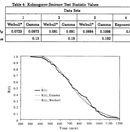
In order to test the goodness of fit, Kolmogorov-Smirnov statistic D r is used. It is defined as [10]

D r = sup IRr(O - RCt)l ,

t

where N is the sample size. The distribution of D r is independent of the cclf F(g) ( = 1 - R(Q) that defines Ho. Accordingly, the acceptance limits for the test of Goodness of Fit are tabulated in [1O, page 580]. The critical region D r > Dr,= is used to test F ( t ) against the alternative that the cdf is not F ( Q , where D r , , is the constant corresponding to the s-significance level a. The values of test statistic are given in Table 4 for all the d a t a sets, for c¢ = .05. W i t h those wlues both Weibull and G a m m a distributions are accepted for the first three sets, and the one whose D r value is smaller, is regarded as the better fitting distribution and marked with a star. With this criterion, in all of them Weibull distribution came out to be better. But we can comment that for the second data set, considering the MRL plot (Figure 4), G a m m a distribution might be preferred, because ~(~) does not decrease, but rather fluctuates after some time, and this obeys to our results for G a m m a distribution in Section 2. In fact, for this set the Kolmogorov- Smirnov test statistics for the two distributions are very close to eachother. Finally, for the last set Exponential distribution is also accepted.

224 M . M . SIDDIQUI and M. (~A(~LAR

We can then, conclude that for the first three data sets, items are aging in

time, and exponential distribution cannot explain the behavior of the bulbs' lifetimes. From the graphs of e(t) versus t, it can be seen t h a t the theoretical curves fit the emprical results, quite well. In relevant situations such as this, M R L function being one of the distribution identities, can also be used as a diagnostic procedure to make a distinction among different distributions, together with the reliability function.

Table 4: K o l m o s o r o v - S m i m o v Test Statistic Values D a t a Sets

1 2 3 4

WeibuU* G a m m a Weibull* G a m m a Weibull* G a m m a Exponential*

DN 0.0723 0.0973 0.081 0.091 0.0884 0.1098 0.0835 D~t,.o5 0.15 0.19 0.192 0.27 0.9 0.8 0.7 0.6 0.5 0.4 - - R(t)_Gamma h~,x~,.~ x , % i 0.3 ... R(t)_Weibull ~ N 0.2 0.1 0 i p i t ~ i i 200 300 400 500 600 700 800 900 1000 1100 1200 Time (rain)

T h e fitted and empirical (R(t)) reliability functions for D a t a Set 1 1. 550 - 500 . . . UB ",, - .... LB 450 , ~ . , "",., ~ ( t ) 400 % " ' - , . \ " ~ - - ~ ""-, ... e(t)_Gamma ~,~ 350 " " ' - , , , , , ~ , _ _ e(t)_Weibull

3oo-_

200 - 150 . . . . 250 300 350 400 450 500 550 600 650 700 750 Time (min)

1.0 -',..., 0.9 0.8 ~ P,(t) 0.7 "~", - - R(t)_Gamma 0.6 ~ ... R(t)_Weibull

" % ,

0.5 0.4 ~ ' ~ ~ 0.3 0.2 0.1 0 ' • - 600 800 1000 1200 1400 1600 1800 2000 2200 2400 2600 Time (h)

empirical (/~(t)) reliability functions for Data Set 2 3. The fitted and

8 5 0 ""~, ... U B ... e(t) G a m m a 8 0 0 "'. "'., ... L B - - e ( t ) _ W e i b u l l 750 ""-, ~ 6(0 700 6 5 0 '"- "- ' " - . " "'. ",., " - 4 "J ". : 600 o) 550 500 450 ,, . . . 400 "', t "-J "-, ,-, 3 5 0 t "'~/ 700 800 900 1000 1100 1200 1300 1400 Time (h)

4. T h e fitted G a m m a a n d Weibull

e(t)

and the empirical ~(t)for D a t a Set 2

1.0 " - . . ~ 0.9 ... ".'.,~, \ , , 0.8 ... ': 0.7 ~ : : ? , 0.6 "' L', .~ o.5 ;~'t" 0.4 - - R(t)_Gamma ~ N 0.20.3 ... R(t) Weibull ~ ) .,,.__~._ 0.1 0 - - 2 4 6 8 10 12 14 16 18 Time (thousands)

226 M . M . SIDDIQU] and M. (~A{~LAR I 0,000

_/

9000 • ~ ' " ' " . r - . - .... UB ... e(t)_Gamma " ' - , - .... LB - - e(t)_Weibull 8000 ~ , . . . . ~ ~(t) j- 7000 "''"'-;--~ 5000 "'"-J"-. ""'""-.. 4000 3000 "'-,. 2000 . . . . . 1000 2000 3000 4000 5000 6000 7000 8000 9000 10,000 T i m e ( h ) 6. T h e f i t t e d G a m m a a n d W e i b u l ] e(~.) a n d t h e e m p i r i c a l ~ ( t ) f o r D a t a S e t 3 1.0 0.9 _E 0.8 0.7 0 . 6 . . .

R(t)

,~ 0.5 ~x', x - - R(t) Exp. 0.4 '~' 0.3 0.2 0.! 0 0 50 100 150 200 250 T i m e 7. T h e f i t t e d a n d e m p i r i c a l ( / ~ ( 0 ) r e l i a b i l i t y f u n c t i o n s f o r D a t a S e t 4 120 110 100 ' ... - ' _._ . . . { 90 / " ... / ... LB ... UB 80 ... 6(t) ~ e(t) Exp. 70 . . , / ... + 60 50 40 ... : ... . ... , 3O

0

;

~;

,;

2o

2;

3b

3;

4;

4;

so

T i m e 8. T h e f i t t e d E x p o n e n t i a l e ( t ) a n d t h e e m p i r i c a l ~ ( t ) f o r D a t a S e t 4

R e f e r e n c e s

[1] M. C. Bryson, M. M. Siddiqui,

J. Amer. Statist. Assn.

64, 1472-1483

(1969).

[2] J. V. Deshpande, et.

at., J. Appl. Probab.

23, 748-758 (1986).

[3] L. M. Leemis,

IEEE T~na. Rel.

R-35, 170-174 (1980).

[4] J. F. Lawless,

Statistical Models and Methods for Life~ime Data,

John

Wiley ~nd Sons, New York (1982).

[5] R. Calabria,G. Pulcini,

Reliab. Eng.

19, 165-170 (1987).

[6] M. Abramowitz; I. A. Stegun,

Handbook of Mathematical FunctionJ,

Dover Publications, Inc., New York (1982).

[7] D. F. Andrews, A. M. Herzberg,

DATA A Collection of Problems from Many Fields for the Student and the Research Worker,

Springer-Verlag,

New York (1985).

[8] D. R. Cox, E. J. Snell,

Applied Statistlcs,

Cambridge University Press,

London (1989).

[9] A. C. Cohen, B. J. Whitten,

Parameter Estimation in Reliability and Life Span Models,

Marcell Dekker Inc., New York (1988).

[10] B.W. Lindgren,

Statistical Theory,

Macmillan Publishing Co. Inc., New