A renormalisation group study of the BNNNI model

J. Phys. A: Math. Gen. 22 (1989) 85-91. Printed in the UK

A renormalisation group study of the

BNNNI

model

M AydinfD and M C Yalabikf

t Mathematics Department, University of Melbourne, Parkville, Victoria 3052, Australia f Physics Department, Bilkent University, Ankara, Turkey

Received 16 March 1988

Abstract. The phase diagram of the two-dimensional biaxially next-nearest-neighbour k i n g ( B N N N I ) model is obtained using the real-space renormalisation group method with the mean-field approximation. The transitions between disordered and commensurate phases are observed to be single transitions for the ferromagnetic phase at intermediate and high temperatures and for the antiphase structure at high temperatures. However, within the approximation, successive transitions are observed between the antiphase structure and disordered phase at intermediate and low temperatures.

1. Introduction

The early studies of the two-dimensional Ising model with competing ferromagnetic and antiferromagnetic interactions created considerable interest in the transitions between commensurate and incommensurate phases. Hornreich et al (1979) studied

the model with competing interactions for uniaxial (known as the A N N N I model) and

biaxial cases using the renormalisation group method with the Migdal-Kadanoff bond-moving as well as Monte Carlo techniques. The phase diagrams of these models display two distinct commensurate low-temperature phases, the ferromagnetic and antiphase structures. In addition, possibly, an incommensurate phase exists at inter- mediate temperatures. Indeed, in the uniaxial case, an incommensurate phase is believed to be present between the disordered and antiphase states (Selke 1981). In the biaxial case, Hornreich et a1 (1979) excluded the existence of such an incommensur- ate phase above the ferromagnetic phase. Selke and Fisher (1980) gave some evidence for an incommensurate phase above the antiphase structure, bounded to the disordered phase possibly by a Kosterlitz-Thouless-type transition. However, Landau and Binder (1985) argued in favour of a direct transition of first order from the antiphase to the disordered phase without any intermediate structure, based on a Monte Carlo study emphasising finite-size effects. Recently, Oitmaa and Velgakis (1987b) studied the two-dimensional Ising model with competing interactions along the two axial directions by series analysis. They saw an indication of a Kosterlitz-Thouless transition between the disordered and antiphase states. They concluded that the absence of a first-order transition supports the existence of two separate transitions, but it is not evident. Oitmaa et a1 (1987) reported an Ising transition in the ferromagnetic region by using finite lattice methods. In the antiphase region, they found distinctive structure in finite lattice estimators at two different temperatures, but they decided that the nature of the transition is not clear. They called the model the biaxially next-nearest-neighbour Ising ( B N N N I ) model. In the latest work by Oitmaa and Velgakis (1987a), the same

8 Present address: School of Physics, The University of New South Wales, Kensington, NSW 2033, Australia. 0305-4470/89/010085

+

07$02.50 @ 1989 IOP Publishing Ltd 85

model has been studied using Monte Carlo methods. They have seen evidence for the existence of modulated structures near the transitions, but the form of the phase diagram remains unclear.

In the present work, the phase diagram of the B N N N I model is obtained by using

the real-space renormalisation group method with the mean-field approximation. The transition between disordered and ferromagnetic phases is observed to be a single transition at intermediate and high temperatures. Along the boundary between dis- ordered and antiphase states, there is a single transition at high temperatures and successive transitions occur at intermediate and low temperatures.

The model and the method are described in

0

2 and the procedure is explained in

0

3. Section 4 includes results and discussions.

2. The model and method

The Hamiltonian, H, of a B N N N I model (Oitmaa et a1 1987) can be described by the expression

where the first summation is over all nearest-neighbour pairs and the second summation is over all axially next-nearest-neighbour pairs of the Ising spins Si ( S , = F 1). K" and K"N are the nearest- and axially next-nearest-neighbour couplings respectively ( K =

J /

kT, J is the magnetic interaction between neighbouring spins, k is the

Boltzmann constant, T is the temperature). The model has one disordered (paramag-

netic) and three ordered (ferromagnetic, antiferromagnetic and antiphase) states. In the present study, the phase diagram of the B N N N I model is obtained using the renormalisation group method (Wilson and Kogut 1974). After the selection of an appropriate cell (which preserves lattice symmetry), the original system is transformed into a new system by a scale change so that a cell in the original lattice corresponds to a new spin in the renormalised lattice. The renormalisation group transformations result in a recursion relation between successive renormalised coupling constants.

A mean-field approximation (Kinzel 1979) is used to obtain the recursion relations.

In this approximation, the Hamiltonian of the system is written in the form

H

Hoi+ V

I

where

and

Here Ho, is an unperturbed Hamiltonian containing the spin products of the cell spins (i.e. the interactions within the cell) and Vis the perturbation containing the interactions between different cells. (The indices i, j are cell indices and U, p are spin indices.) The spin products S,,S,, can be written as

Renormalisation group study of B N N N I model 87

where ( S i " ) is assumed neglected.

denotes the average or mean-field value of the spin s i v . If the mean value to be equal to the value of the spin, the first term in equation (5) can be Using equation (5), the mean-field value V M F can be written as

where mi, mJ are the average values of the spins SI, S, respectively and the summations are over all cell interactions.

The free energy of the system can be calculated using the partition function, which is

2 = exp( - H { S}/ k T ) (8)

1s)

where the summation is over all possible spin states. After the first renormalisation group transformation, the number of spins N in the original system is reduced by a

factor b, where J b is the scale change of the transformation. The number of spins N ' in the renormalised lattice is given by

N ' = N / b . (9)

Z = exp[-H'{S'}/ k T + ( N / b ) K b ] (10)

The partition function of the renormalised system can be described by the expression

{ S ' )

where Kb is the constant appearing after the first renormalisation. After n transforma- tions, the partition function will be in the form

2 =

exp[-H""'(S''"'}/kT+(N/b")K~].

i s 1

(11) If n is sufficiently large, the first exponential term will be small compared with the second term and can be ignored. Then Z will have the form

exp[( N / b")Kb'"']. (12)

(13)

(14)

z

= 2N/bn

The free energy, f, per spin can be calculated from equation (12) using the relation

- f / k T = (1/N) In Z

-

f/

kT

= (In 2

+

Kb("')/ b

".

and is given as

3. The procedure

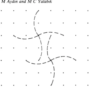
Computations are carried out for a single cell on a square lattice. The form of the selected cell is given in figure 1. The coupling constants K" and K"N are given initial values and the system is renormalised into a new system in which five spins of

I

' I

Figure 1. The form of the selected cell for two different sublattices.

the cell correspond to a new spin ( b = 5). The state of the new spin is determined by the majority rule. Depending on the values of initial couplings, renormalisation group trajectories end either at the high-temperature fixed point in the disordered phase or at a low-temperature fixed point in one of the ordered phases. Figure 2 shows one possible ground state for the antiphase state.

The Hamiltonian contains the average values of the spins included in the interactions between cells. The average value of the spins can be evaluated for the three ground states using the relation

Here 1 is used to label the ordered ground states of the system and j is used to label the spins having different symmetry in the lattice. HI{ S} is the approximate Hamiltonian with the mean-field term for the lth ground state (which itself is a function of mil).

Starting with an initial value (e.g. m,, = 1) the average value of the spin can be obtained by successive substitutions of m,/ into the expression given in equation (15). The

iteration is stopped when the difference of the two last iterations is small compared

Figure 2. One possible ground state for the antiphase state (called the checkerboard or chessboard state).

Renormalisation group study of B N N N I model 89

with the value of mj,. Once the mil are determined, the values of H' for the three

ground-state configurations can be determined. The renormalised Hamiltonian can be written as

where K

h N

and K

h"

are the renormalised nearest- and next-nearest-neighbour coupling constants respectively. Kb, Ki\lN and Kh" are three unknowns which can be found from the three equations resulting from equation (16). The constant Kb is

used to calculate the free energy as explained in § 2. The RG trajectories are obtained

using the values of K

hN

and K

h N N

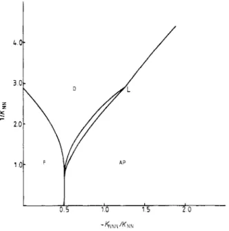
after each RG transformation for different initial

couplings. The resulting phase diagram is shown in figure 3. For convenience, 1/KNu free energy (through the variation of K b ) is studied carefully to confirm the positions of all phase boundaries.

(i.e. kT/J") iS plotted as a function Of -K"N/K" (i.e. -J"N/J"). Variation O f

I I

0 5 1 0 1 5 20

-

KNN N /KN N

Figure 3. The phase diagram of the B N N N I model as a result of RG trajectories ( D =

disordered phase, F = ferromagnetic phase, A P = antiphase state).

4. Results and discussion

The phase diagram of the B N N N I model is obtained by using the RG method with the

mean-field approximation. When the nearest-neighbour coupling is zero (i.e. K" = 0) this model reduces to an Ising model with a critical coupling K Z N N = 0.43. For zero next-nearest-neighbour coupling (i.e. K"N = 0), K G , = 0.32 is the critical coupling in the ferromagnetic region. The exact critical value for the two-dimensional Ising model is K C = 0.4407..

.

.

The large discrepancy between KZN and K C may be due

As a result of RG iterations, the transition between ferromagnetic and disordered

phases is observed to be a single transition. But the transition between the disordered and antiphase states show different characteristics in two different ranges of K,,

values. Calculations with various numbers of RG transformations show that, for the

values of KSN

<

0.32, there is always a single transition between the two phases. For larger values, disordered and antiphase states appear successively for a range of K N N N values at fixed KNN. (Actually, because of numerical difficulties, we have not been able to see these successive phases in the region 0.32 G K N N < 0.38. However, our data

suggest that this region extends down to KNN = 0.32.) At low temperatures, successive (ferromagnetic-disordered phiise) transitions are observed along the boundary between the ferromagnetic and disordered phases.

It should be mentioned that the phase structure with successive transitions (corre- sponding to the phases associated with two fixed points) cannot be obtained through the standard renormalisation group trajectory analysis. In this computation, the poss- ible existence of a different type of order in the system (whose ground state is not conserved by our RG transformation) seems to yield a chaotic structure in the renormali- sation group trajectories that start from points corresponding to this type of order. The region including successive transitions supports the existence of an incommensur- ate phase between the disordered phase and antiphase state. It is strongly evident that there is a single transition between these phases for the values of K,, < 0.38 and that there exists another phase between these phases for larger values of K N N . (This suggests the existence of a corresponding Lifshitz point at K N N = 0.38 F 0.07 and KNNN = -0.42r0.02, the point L in figure 3.) To our knowledge, there is no other study which indicates the presence of a phase corresponding to the successive ferromag- netic-disordered phase transitions that we see at low temperatures.

1 0 2 0 3 0 4 0

-

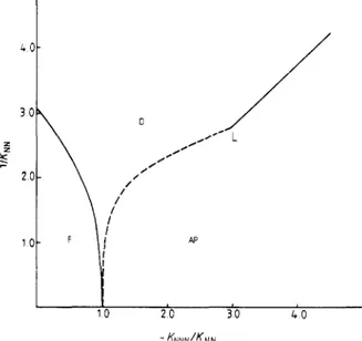
KNNN/KNN

Figure 4. The phase diagram of the A N N N I model as a result of RG trajectories. ( D =

disordered phase, F = ferromagnetic phase, A P = antiphase state.) The full curves represent king-like transitions; the broken curve marks the boundary of the successive transition region.

Renormalisation group study of B N N N I model 91 When calculations are repeated for the uniaxial case, the critical coupling for K"N = 0 is obtained as K g N = 0.32, which is exactly the same as that for the B N N N I

model. For KNN = 0, the model decomposes into uncoupled one-dimensional Ising models. One would therefore expect an infinitely large critical magnitude for K"N. However, the mean-field approximation results in the finite value KN" = -1.05.

The phase diagram of the A N N N I model has the same characteristics as those of

the B N N N I model (figure 4). The appearance of successive transitions at an intermediate

temperature can be considered as evidence of a Lifshitz point (the point L in figure

4) at K" = 0.36F0.04 and K"N = -1.07T0.10. The transition points are obtained with the same accuracy achieved for the B N N N I model except at the boundary between the successive transition region and antiphase state. It was not possible to obtain this boundary accurately in the uniaxial case due to computational difficulties. Some of the RG trajectories which start from the successive transition region pass through points

where K" < 0. This may be the indication of floating phases which are not observed for the B N N N I model. The successive transitions appearing at low temperatures along

the ferromagnetic-disordered phase boundary of the B N N N I model are not observed

in the uniaxial case.

This method is not expected to give very accurate results in calculating numerical values (because of the mean-field approximation). However, the general features of the resulting phase diagrams are expected to be correct.

Acknowledgments

The authors would like to thank W Selke for valuable discussions. They also thank P A Pearce for his encouragement to complete the work. This research was supported in part by a grant from the Australian Research Grants Scheme.

References

Hornreich R M , Liebmann R, Schuster H G and Selke W 1979 Z. Phys. B 35 91 Kinzel W 1979 Phys. Rev. B 19 4584

Landau D P and Binder K 1985 Phys. Rev. B 31 5946

Oitmaa J, Batchelor M T and Barber M N 1987 J. Phys. A: Math. Gen. 20 1507 Oitmaa J and Velgakis M J 1987a J. Phys. A: Math. G e n . 20 1495

- 1987b J. Phys. A : Math. G e n . 20 1269 Selke W 1981 2. Phys. B 43 335

Selke W and Fisher M E 1980 2. Phys. B 40 71 Wilson K G and Kogut J 1974 Phys. Rep. 12 77