: G ölíУ ■P F tE 'SSiufí■’^0’F' ;ώ T O τ κ : £ · О‘0?'/О гХ х«Е ічГ Г •■.‘ ч '■νΤ··'":'^·,’ ·*^·~·<'·'Т?Г:3“ '7Т:і· ‘ Vu’T'·· !:ír» ■ Т"·· *т ■’? •^‘і ν ' \ « r n t '■'>■· •*’J ' * ’ ·- ·<·>·;( . ■ ■.. · ν · · : ί · Λ . . г·. -* Г'·' - Λ··: 'ГП> · ν ·; V··^ ' T ■ ·'7*^-··’ * ' ■ ■ ’’* V·.’^^··-'‘••'■^■•7 r·^··:*': **^·:.*·'"'Γ·*·'*7 ... ^ · . ‘. и-Тч^і ·:/ -Ьосоо· о о " **“ я· τ η / ( ? 3 7
Τ/1 ibZ'-l·
y J
LOSSLESS COMPRESSION OF MEDICAL IMAGES
A T H E S IS S U B M I T T E D T O T H E D E P A R T M E N T O F E L E C T R I C A L A N D E L E C T R O N IC S E N G IN E E R IN G A N D T H E I N S T I T U T E O F E N G IN E E R IN G A N D S C IE N C E S O F B IL K E N T U N I V E R S I T Y IN P A R T I A L F U L F IL L M E N T O F T H E R E Q U IR E M E N T S F O R T H E D E G R E E O F M A S T E R O F S C IE N C EBy
Behiç Fırat Kılıç
July 1991
.. FirQl-
-till·
I certify that I have read this thesis and that in my opinion it is fully adequate, in scope and in quality, as a thesis for the degree of Mcister of Science.
< k
c?
Assoc. Prof. Dr. Ahmet Enis Çetin(Principal Advisor)
I certify that I have read this thesis and that in my opinion it is fully adequate, in scope and in qualitj>·, as a thesis for the degree of Master of Science.
Assoc. Prof. Dr. Mehmet Ali Tan
I certify that I have read this thesis and that in my opinion it is fully adequate, in scope and in quality, as a thesis for the degree of Master of Science.
Approved for the Institute of Engineering and Sciences:
____________________ ■ ■
-Prof^ Dr. Mehmet B a r a y ^
ABSTRACT
LOSSLESS COMPRESSION OF MEDICAL IMAGES
Belıiç Fırat Kılıç
M.S. in Electrical and Electronics Engineering
Supervisor; Assoc. Prof. Dr. Ahmet Enis Çetin
July 1991
The digital imaging techniques are used more and more in various diag nostic modalities, including computed tomography (C T ), Digital Subtraction .A.ngiography (DSA), etc. As a result, a huge amount of digital images are being generated. Therefore, techniques to compress these images into a more compact form for storage and transmission become more important and anyone involved with the storage of medical images in a Picture Archiving and Com munication System (PACS) should first apply compression (lossy or lossless depending on the characteristics of the digitized data) on them. There are im age coding methods which reduces the storage size of an image b}' an amount of 1/10 without any visual degradation. But in some medical applications lossless coding of medical images is necessary.
Multiresolution coding techniques have been used for lossy image and speech coding, in this thesis we developed multiresolution techniques for the lossless image compression. We observed that the use of multiresolution techniques in lossless compression is as advantages as in lossy compression schemes.
ÖZET
MEDIKAL
g ö r ü n t ü l e r i nKAYIPSIZ OLARAK
SAKLANMASI
Behiç Fırat Kılıç
Elektrik ve Elektronik Mülıendisliği Bölümü Yüksek Lisans
Tez Yöneticisi: Doç Dr. Ahmet Enis Çetin
Temmuz 1991
Sayısal görüntüleme tekniklerinin tomografi, anjiografi vs. gibi alanlarda her geçen gün daha fazla kullanılmaya başlanmasıyla, çok fazla yer kaplayan medikal görüntülerin saklanması önemli bir sorun olmuştur. Bu görüntülerin daha yoğun bir şekilde saklanmasını sağlayan teknikler de önem kazanmıştır. Bazı geliştirilen az kayıplı metodlarla bu görüntülerin kapladığı hafıza 1/10 oranında azaltılabilir. Fakat, medikal alandaki bazı kullanımlardan dolayı hiç kayıpsız saklama önemli bir araştırma alanı olarak kalmı.ştır.
Bugüne kadar çok çözünüldü teknikler kayıplı saklamalarda kullanım alanı bulmuştur. Bu tezde ise çok çözünüldü teknikler kayıpsız görüntü saklamasında kullanıldı. Çok çözünüldü tekniklerin, en az kayıplı saklamada olduğu kadar kayıpsız saklama alanında da başarılı olabileceği yapılan deneylerle de gözlendi.
ACKNOWLEDGMENT
My first debt is to Assoc. Prof. Dr. A .Enis Çetin who provided perfect dosage of criticism and unfailing support throughout the project.
A special note of thanks is to my father and mother who are the real supporters of my studies in Bilkent University.
Finally I should like to thank to all my friends, primarily to Erkan .Savran and Atilla Malaş, in the University who have one way or another participated, helped or supported me all through my MS work.
Contents
1 Introduction 1
1.1 In trodu ction ... 1
2 An Overview of Some Multirate Techniques 3 2.1 In trodu ction ... 3
2.1.1 Subband D e co m p o sitio n ... 4
2.1.2 Pyramidal D e c o m p o s itio n ... 14
3 Review of Some Waveform Coding M ethods 16 3.1 In trodu ction ... 16
3.1.1 Transform Domain C o d in g ... 17
3.1.2 The Huffman C o d in g ... 22
3.1.3 Run-length C o d i n g ... 24
4 Lossless Multirate Image Coding 26 4.1 Introduction to Subband C odin g... 26
4.1.1 Coding with nonrectangular subband decomposition . . . 27
4.1.2 Coding with rectangular subband decom position... 30
4.1.3 Pyramidal Coding 31 4.2 C onclusion... 34
List of Figures
2.1 X(e^^') is the shifted and scaled sum of A’a (iil) 4
2.2 Interpolation o p e ra tio n ... 5
2.3 Decimation opera tion ... 6
2.4 Subband decomposition by 2 ... 7
2.5 Ideal subband decomposition s t r u c tu r e ... . . ,... 7
2.6 Cuin-cunx downsampling s t r u c t u r e ... 10
2.7 Nonrectangular subband decom position... 11
2.8 Reconstruction stage for nonrectangular d e co m p o sitio n ... 12
2.9 Rectangular subband decom position... 13
2.10 Reconstruction stage for rectangular d e co m p o sitio n ... 14
2.11 The pyramidal coding s t a g e ... 15
2.12 Reconstruction stage of the pyramidal c o d e r ... 15
3.1 Reconstruction of the image from bcisis im a g es... 18
3.2 Zig-zag s c a n ... 21
3.3 Huffman codebook for the DCT a lg o r ith m ... 22
3.4 Optimum code assignment p r o c e d u r e ... 23
3.5 Modified Huffman codebook pair 24
LIST OF FIGURES viii
4.1 Code book for low information s u b -im a g e s... 27
4.2 DCT coding structure ...28
4.3 Pyramidal coding with lossy D C T ... 32
4.4 The sample image “Angio” ... 33
List of Tables
4.1 D C T based results for nonrectangulcir decomposition 29 4.2 Difference based results for nonrecrangular decomposition . . . . 30 4.3 D C T based results for rectangular decomposition 31 4.4 Difference based results for rectangular decom position... 31 4.5 Pyramidal compression resu lts... 33
Chapter 1
Introduction
1.1
Introduction
The digital imaging techniques such as Computed Tomography (C T ), Digital Subtraction Angiography (DSA), ultrasound, nuclear medicine and computed radiography are used increasingly in various diagnostic modalities. Therefore, a huge amount of digital images are being generated, for which compression into a more compact form for storage and transmission become more important.
Medical images are usually digitized in large rasters. For instance, a chest X-Ray is scanned in a raster of size 2048 lines and 2048 columns (or 1024 x 1024 in some cases) with pixel depth of 12 bits and digital subtraction angiogrciphy (DSA) images are digital images of size 512x512 (in most machines) with pixel depth ranging from 8 bits to 12 bits. These figures stress the fact that, any type of image consumes a huge amount of storage media. Furthermore, if we consider storing huge amount of medical images in a hospital Picture Archiving and Communication System (PACS) the importance of the data compression becomes even clearer. Hence, anyone involved with the storage of mediccil images in an archive or the transmission via a telecommunication system should first apply compression (lossy or lossless depending on the characteristics of the digitized data) on them. We believe that the image compression unit must be an integral part of any PACS [2].
CHAPTER 1. INTRODUCTION
Image compression methods can be classified into two main categories: Lossy (irreversible) and lossless (error-free) coding methods. Although the techniques developed in this thesis can be applied to all kinds of images, we will be mostly concerned with error-free (lossless) coding of medical images due to legal reasons commonly used; lossy image coding methods can not be used in compressing medical images.
Many irreversible image coding techniques have been developed during the past two decades for applications ranging from tele-conferencing to the trans mission of digital T V images [7],[8]. Recently, multiresolution image coding techniques become popular [4]-[7]. In gray-scale High Definition Television (HDTV) images a comiDression ratio of three can be achieved without intro ducing any visual degradation using multiresolution image coding (in fact some HDT\' standard proposals are based on multiresolution image coding) and for other images compression ratios of as high as ten can be achieved by using mul tiresolution coding methods. However it should be noted that, visually lossless is a term to describe a lossy coding technique in which the reconstructed image is visually indistinguishable. As the name irreversible implies some numerical loss on the image pixel values are introduced in the irreversible coding. In some medical applications any loss however harmless it may seem may not be tolerable. Therefore, in these cases medical images should be compressed by numerically lossless image coding techniques. In this thesis we developed multiresolution lossless image compression methods for medical images.
Most of the lossless techniques are based on a lossy technique plus an error- correction unit. So, we will first examine lossy techniciues in order to extend the study to lossless cases, as well.
We also review multirate signal processing, transform domain coding, Huff man coding, run-length codirrg etc. in Chapters 2 and 3. These concej^ts are extensively used in our coding schemes. In Chapter 4 we present the newly developed multiresolution medical image coding methods and some simulation examples.
Chapter 2
An Overview of Some Multirate Techniques
2.1
Introduction
The key idea of multirate signal processing (MSP) based coding methods is to represent the signal in lower resolutions, and to encode each of these com ponents separately. By dividing the signal into sub-signals we wish to remove redundancies and obtain a number of uncorrelated sub-signals.
These uncorrelated sub-signals can be coded more efficiently than the cor related ones [14], [15]. Indeed, optimum coding can be achieved if the signal can be decomposed into perfectly uncorrelated sub-signals [16].
In our case, the signals will be two dimensional and Avill be referred as images. The decomposition of images to several sub-images in lower resolutions has the advantage that, the number of bits used to encode a sub-image which corresponds to a frequency component of the original image can be variable. So, the encoding accuracy is always placed wherever it is needed in the frequency domain. In fact, bands with little or no energy may not be encoded at all in some lossy coding techniques.
The rest of this section describes two multirate signal processing techniques which are subband and pyramidal decomposition methods.
CHAPTER 2. AN OVERVIEW OF SOME MULTIRATE TECHNIQUES
4
Figure 2.1: A'(e·’^) is the shifted and scaled sum of XaiJO.)
2.1.1
Subband Decomposition
Let us assume that we have a bandlimited analogue signal Xa{t) with the con tinuous time Fourier transform (C TFT)
Xa{t) XaijO)
(
2
.
1
)
It is well known from the Nyquist theorem that the discrete time Fourier trans form (D TFT) of the signal Xa{nTs) is given as follows^
:.(nr.)'Si? A V ”) =
k=—oo s Ts
(
2
.
2
)
In Fig.2.1 we plot X{e^'^) and Xa{jO) where D TFT X{e^^) of the analog signal Xa{t) sampled at nT^ intervals is the shifted and scaled sum of it’s CTFT XaUn).
Note that H = lo/Ts and Tj = 1 / / , in Fig.2.1. Aliasing occurs if sampling rate is lower than the Nyquist rate.
Having mentioned the frequency domain behavior of a bandlimited signal under sampling we can introduce the concept of digital decimation and digital interpolation.
T h e d igita l in te r p o la tio n by a factor of L is the operation of padding L-1 zeros between the consecutive samples of the time domain signal x[n) and then
CHAPTER 2. AN OVERVIEW OF SOME MULTIRATE TECHNIQUES
5
jw x(n) raicf 1 2 3 4 5 6 7 8 JW-e-e-
-B-e-Figure 2.2: Interpolation operation
JW
X (n) 1 x(n)
0
♦ 1
rate Lfs ^ /l raioLfs
filtering it with a low-pass filter cut-off at tt/L . Padding L-1 zeros increases the rate by a factor of L and represented by the symbol L | to indicate an increase in rate by a factor of L This increase in the rate causes a proportional redundancy in the frequency content of the signal. The original signal can exactly be extracted from its’ aliases by low-pciss filtering with cut off tt/L . The described operation of interpolation (both in time and frequencj'· domain) can be summarized by the Fig.2.2. Note that in Fig.2.2 the zero padded signal X ,(e·’ “') can be represented in terms of the input signal as follows^:
AT(e'·^) = X{e^^^) (2.3)
T h e digital d e c im a tio n is a complementary operation of the digital inter polation. That is, if certain constraints are satisfied a decimated signal can exactly be reconstructed by interpolation. In decimation, rate of the signal is reduced by a factor of M and represented by M J, . We filter the signal by a low-pass filter at cut-off tt/ M and drop M -1 samples out of every M samples“’ . Prefiltering by a low-pass filter (sometimes called the decimation filter) with cut off at 7t/ M avoids the possibility of aliasing which may occur after decima tion. Unlike to interpolation, decimation operation increases the bandwidth of the signal and may cause aliasing. The decimation operation (both in time and frequency domain behavior) can be seen in Fig.2.3.
^This is known as “upsampling” ^It is assumed that wq < tt in Fig.2.2 ^This is known as “downsampling”
CHAPTER 2. AN OVERVIEW OF SOME MULTIRATE TECHNIQUES
6
jw InputУ
4
^
ifM = 3 1 2 3 4 5 6 7Figure 2.3: Decimation operation
Also note that
1_
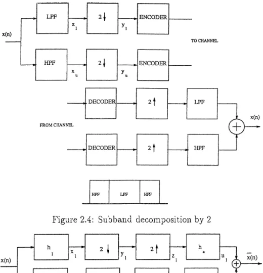
M M-l • w-2nkЧ e*' M ) k=0 (2.4)In subband decomposition the input signal is decomposed to sub-signals in lower resolutions according to their frequency contents. A typical subband decomposition structure is shown in Fig.2.4.
This structure decomposes the input signal x{n) into two sub-signals xi and Xu- After decimation by 2 (i.e., 2 |), these two sub-signals are fed into the encoder and then to the channel. The receiver decodes the received signal and interpolates it. In this way, the input signal x{n) can be reconstructed at the receiver.
Now let us derive the necessary conditions on the filters (in Bhg.2.4) for excict reconstruction of the signal at the receiver part. Бог this purpose we will exclude the encoder,decoder and the channel. The structure will be as in Fig.2.5.
The formulation of the subband structure (in Fig.2.5) begins as follows:
from Eq.2.4
(2.6)
X„(e^·"') = Я „(е> )Х (е^ ·” ) (2.6)
ï)(e ’ ” ) = i [ X ( e 'ï ) + A ', ( e '4 = ^ ) l (2.7)
CHAPTER 2. AN OVERVIEW OF SOME MULTIRATE TECHNIQUES
7
Figure 2.4: Subband decomposition by 2
Figure 2.5: Ideal subband decomposition structure
and from Eq.2.3
1
The output is where Z j e n ^ y;(e^'2“ ) = - [ X u ( e n + = Uiie^·^) + U u { t ^ = //b(e>)^[A:„(e^"^) + A'4e^(“'+"))] (2.9) (2.10) (2
.11
)(
2
.
12
)
(2.13) (2.14) (2.15)CHAPTER 2. AN OVERVIEW OF SOME MULTIRATE TECHNIQUES 8
inserting and Xu{e^'^) values (Equations 2.5,2.6) we get
(2.16)
L\{e^^) = - ^ ^ - \ lR{e^'^')X{e^'^) + ii„(e^’(“'+^))X(e^>+’^))] (2.17)
so the output is
X{ e
l'u^\ —
X { e N ) [IU{enHi{e^'^) + ii6 (e^ -)//„(e^ -)] A2(ei'‘A(e^'“ ) =
(2.19)By examining Eq.2.19 we observe that, the output is composed of two terms where is an aliasing term which should be canceled for exact reconstruction of A'(e·^“') at the output.
In order to reconstruct the input signal at the output of the subband de composition structure we need to have:
1
) Ai(e·^^) = where 6^°'^ only introduces a time delay of ko units; and2) A'ife·^'^) = 0 to cancel the aliasing term.
There are many filter design algorithms [3]-[5],[10],[ll] to satisfy these condi tions and hence, reproduce exact replica of x{n) at the receiver.
One such design with FIR filters is obtained as follows:
• Choose hi[n) of order N (N is even) linear phase FIR low pass filter®. • Choose hu{n) — ( - l ) ” /i;(?r). ®
SNote hi{n) = hi{N - n - 1) => f/fie^'“') = \Hi{U'^)\^
CHAPTER 2. AN OVERVIEW OF SOME MULTIRATE TECHNIQUES
9
It can be easily shown that = Hi(eA^+^)J with the above choice of the filters.
Finally choose
which implies that A2(e^'“') = = 2H,(e^^) and = -2Hu{e^'^)
0
J W \(2.20)
(
2.21)
(2
.22
) (2.2.3) (2.24) and note that so ifAi(e^'"') -
Hi{e^^)Ha{e^'^) P Hk{e^'^)l·h{e^'^)(2.25)
=
Hi{e^'^)2Hi{e^'^) - 2Hu{e^")IL{e^^)(2.26)
=
2[Hi{e^'^f - Hu{e^'^f\(2.27)
Hi{t^'^f = \Hi{e^'^)\^
(2.28)
= _ |F/,(e-''(“+^))|^e“^'“'(^“^)
(2.29)
Ai(e^'“') = 2[|/7,(e^'^")f + |77,(e^'(“^+^))f
(2.30)
|Ff,(e^'"’)p + |i/,(e'(“'+’^^)|" - 1
(2.31)
then we satisfy the exact reconstruction condition.
One dimensional (1-D) subband decomposition structures can be general ized to two dimensions (2-D) in many ways [7]. VVe now consider two different subband decomposition methods to decompose the image into sub-images at different resolutions. In the first method, we use diamond shaped exact recon struction filter banks [4],[11] and in the second one we use rectangular exact reconstruction filter banks [5],[9],[10].
CHAPTER 2. AN OVERVIEW OF SOME MULTIRATE TECHNIQUESlO o o o o o o o o o o o o o o o o o o o o o o o o o o o o o o o o o o o o Q Q O -e - O Q O Q O o o o o o o o o o o o o x(n) o o o o o o o o o o o o o o o o o o o o o o o o o o o o
Figure 2.6: Cuin-cunx downsampling structure
N o n r e cta n g u la r S u b b a n d D e c o m p o s itio n
The nonrectangular decomposition is a subband decomposition method where nonrectangular filters are used for separation of the input image into sub-images (see Fig.2.7). The simplest way is the separable 2-D filters where the filters are constructed from 1-D filters such that;
Hij{wi,W2) = Hj {1Ü2) (2.32)
But other non-separable 2-D structures can also be used. Apart .from filters the decimation and interpolation operations can also be generalized to the 2-D case in the same manner. This time decimation and interpolation factors M and L, respectively turn into matrices. The sampling rate is either decreased or increased by a factor of |dei(M)| or |dei(L)|, respectively. A simple decimation operation by a factor of M in 2-D space can be seen in Fig.2.6 where
M = 1 1
1 -1
(2.33)In Fig.2.6 y{n) — x ( M n). This decimation scheme is also known as the “quin-cunx” downsampling where only half of the samples are retained and the rest is dropped [17].
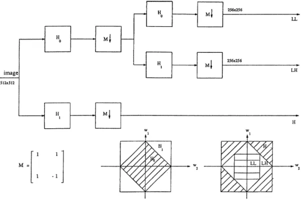
Our nonrectangular subband decomposition scheme consists of two stages. In the first stage the medical image is filtered by two filters. One of these filters is a lowpass filter with a diamond shaped' passband. The other filter is a high pass filter with a diamond shaped stopband. The outputs of these filters are downsampled by a factor of 2 on a line quin-cunx grid. In this way two sub-images are obtained. The sub-image coming from the lowpass filter is decomposed and downsampled once again by the same filterbank. In effect
^Among many other possible nonrectangular filter structures “diamond shape” is a spe cific filter (see Fig.2.7) which we used in our simulations.
CHAPTER 2. AN OVERVIEW OF SOME MULTIRATE TECHNIQUESll
Figure 2.7: Nonrectangular subband decomposition
the procedure splits the image information into three regions in the frecpiency domain, ideally as shown in Fig.2.7. In this way a low resolution sub-image LL and two dilference sub-images (LH and H) are obtained from the original image.
In Chapter 3 we make use of the special characteristics of these sub-images in our coding algorithms to lower bitrate or equivalently to improve data com pression.
In order to perform the multiresolution subband decomposition the follow ing HR filters described in [4] are used:
= ^ + 2{-iye^^^T{io,+U2)T{u, - C02), 1 = 0,1 (2.34) where
n . ) = ‘ (2.35)
2 ■ 1/3
-f-is an all-pass section. The filter with subscript i = 0 (i = 1) -f-is the lowpass (highpass) filter. In order to reconstruct the coded image from the sub-images the synthesis filter bank of [4]
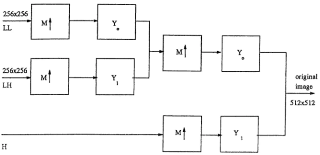
Yi{wi,W2) = 2 H i { - W i , - W 2 ) , i = 0 , l (2.36) which provides exact reconstruction is used. The reconstruction structure can be seen in Fig.2.8.
CHAPTER 2. AN OVERVIEW OF SOME MULTIRATE TECHNIQUES12
Figure 2.8: Reconstruction stage for nonrectangular decomposition
During this process no loss is introduced by the chosen filter bank of [4]. Hence, by the proper choice of filter bank the frequency content of the im age can be split into lower resolutions and then can be reconstructed again without any distortion. This method is called as the nonrectangular subband decomposition.
Rectangular Subband Decomposition
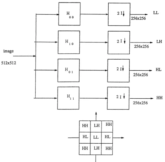
The second subband decomposition method which we consider is the well known rectangular decomposition method [3],[6]. It is another subband de composition method in which exact reconstruction filters of rectangular shape (see Fig.2.9) are used.
A splitting ¡procedure similar to the nonrectangular case is applied to the image. But this time, the filters in the structure are rectangular cind instead of applying a tree like structure for decomposition we use the structure shown in Fig.2.9. The image is split into 4 sub-images instead of three as in the case of nonrectangular subband decomposition.
In our work, we use the separable IIR*^ filter bank of [5] which introduce no loss to the image. The filters used are
(2.37)
where
i / i H = -[1 + ( - l ) V " T{2u,)l
(2.38)
CHAPTER 2. AN OVERVIEW OF SOME MULTIRATE TECHNIQUES13 LL LH HL HH and
Figure 2.9: Rectangular subband decomposition
+ 1 r ( 2 c )
1 /3 + (2.39)
The low resolution sub-image (LL in Fig.2.9) carries the highest information among other sub-images LH, HL, HH. Later on, this property will be e.xploited to improve the compression ratios of the images.
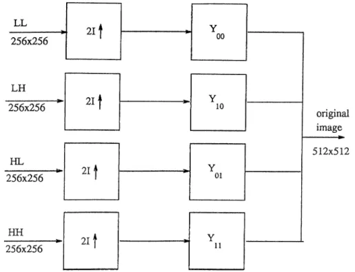
Reconstruction of the original image from the sub-images is carried out by the synthesis filter bank of [51
i-;W = j ( l + (-!)' r(-2«;)], ! = 0,1
with the reconstruction structure of Fig.2.10.
(2.40)
These decompositions of the image into sub-images (either rectangular or nonrectangular) enable us to make use of particular code-books to encode par ticular frequency ranges. As it will be discussed in detail later on, this improves data compression.
CHAPTER 2. AN OVERVIEW OF SOME MULTIRATE TECHNIQUESli
Figure 2.10: Reconstruction stage for rectangular decomposition
2,1.2
Pyramidal Decomposition
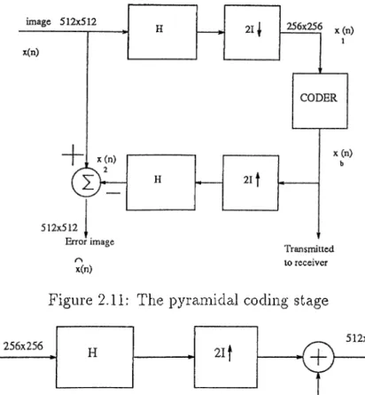
Pyramidal decomposition is another multirate signal decomposition scheme. A typical pyramidal coding structure is shown in Fig.2.11.
The image a;(n) (where .x’(n) = a;(ni,n2)) is filtered and down sampled, on a rectangular grid, to a;i(n) where the number of pixels are reduced by a factor of 4 during the process^. The image a;i(n) corresponds to the low frequency range hence, carries more information. After it is being coded this quantized and encoded sub-image a,’6(n) is then upsampled and interpolated to form a;2(n) (which is of the original image size). Then the error image ;r(n), is obtained by subtracting the reconstructed image o:2(n) from the original image o:(n), i.e. ,
.r’(n) = ,T(n) - 0:2(11) (2.41)
This completes one full cycle through the pyramidal structure. The error image a;(n), is either entered to a similar structure once more or transmitted to the receiver after being quantized and coded.
Pyramidal decomposition structure produces samples (5/4 times) more than the input image sarhples whereas in subband decomposition structures
®H is a separable 2-D Lagrange filter o f length 7 and 21 j is a rectangular
' 1 0 “
downsampling matrix / =
CHAPTER 2. AN OVERVIEW OF SOME MULTIRATE TECHNIQUES 15
x(n ) b
^n)
x(n) lo receiver
Figure 2.11: The pyramidal coding stage
x(n)
Error image
Figure 2.12: Reconstruction stage of the pyramidal coder
the number of output samples are equal to the input samples. The pyramidal structure is suitable for compression purposes as the error sequence x’ (n) which is of the original image size carries very low information.
The receiver part of the pyramidal coder is shown in Fig.2.12. The recon struction is error free without considering the transmission errors that may occur in the channel.
Chapter 3
Review of Some Waveform Coding Methods
3.1
Introduction
The main purpose of any image coding method is to reduce the redundancies in the image as much as possible so that one either communicates in lower bit rates or stores the image in less memory. We try to assign symbols to pixels in an image, in such a way that we achieve this goal.
Image coding methods can be classified in tAvo main categories; irreversible (lossy) coding and lossless coding. Irreversible coding methods add distortion to the image during the compression of the data which can not be exactly recovered afterwards. That is, some amount of information is lost forever. The amount of information loss during the process also determines the amount of compression. The more information (visual qualit}'·) one loses the more compression one gets. Depending on the technique used, the relation between these two criteria difldr. That is, for one method one loses to much from visual quality to reach a certain compression ratio where as for another one does not lose that much from visual quality (information) to reach the same compression ratio. The aim is to achieve visuall)'^ lossless images with minimum loss of information.
In lossy image compression visual quality is a vital criteria. Hence there has to be an objective measure to decide on the distortion introduced to the image. Although there is not yet such a mathematical expression which is in full correlation with the human visual system, there are still expressions that somehow give a measure of the quality of the restored image. This way, we use both subjective measures as well as the objective ones to indicate the visual quality of the image.
CHAPTER 3. REVIEW OF SOME WAVEFORM CODING METHODS
17
Some very common objective distortion measures are
E [ x ( n ) -iV2 M.S.E. M S E ^ MSEdh = - 2 0 Locjw ( ^ [ x ( n ) - y(n)]2 . / y7[x(n)-v(n)P V m
)
(3.1) (3.2) (3.3) where x(n ) and p(n) are input and output images to the image compression scheme, respectively and is the dimension of the images. The summations are over all image and x(n)„гαa: is the maximum gray-level value of the input image.In lossless coding, however, there is no loss at all. That is all the gray-level values of the image are restored back exactly. The problem in lossless coding is to propose such a method that a considerable compression can.be achieved while no distortion is introduced at all.
In the next sections we introduce some coding strategies which we exten sively use in our image compression schemes.
3.1.1
Transform Domain Coding
The term image transform usually refers to a class of unitary matrices for rep resenting images [7]. Just as a 1-D signal can be represented by an orthogonal series of basis functions, an image can also be represented in terms of a discrete set of basis arrays called basis images. These basis images can be generated by unitary matrices.
A unitary transform is represented by a matrix, A. The transform y of a 1-D sequence { ti(n), 0 < < A'' — 1 } is given by
N - l
V = All = > v{k) = ^ a[k,n)u{n), 0 < k < N — 1 (3.4)
n=0
where A~^ = A*'^ (as in all unitary transforms) then
N - l
u — A*^v u{n) = v{k)a*{k, n), — 1 (3.5) k=0
The columns of A*^ are called the basis vectors of A. Depending on the trans formation used these basis vectors differ.
CHAPTER 3. REVIEW OF SOME WAVEFORM CODING METHODS
18
Figure 3.1: Reconstruction of the image from basis images
In 2-D the situation is quite similar and an image of size vV x N can be represented by the transformation of the form
N - i N_i v{k,l) =
EE
u{rn,n)ak,t(m,n) , 0 < k,l < N — 1 (3.6) and m = 0 n = 0 N - l N - 1 u{ m, n) = , 0 < m , n < N — l (3.7) k= 0 1=0where ak,i{m,n) is a set of complete orthonormal discrete basis functions sat isfying the properties
i) Orthonormality ak,i{m,n)al,,,{m,n) S{k - k',l - I')
ii) Completeness Yk=o (‘'k,tim,n)al i{m',n') = 8{m — m',n — n')
Most of the unitary transforms used in image processing are separable that is. Uk,i{m,n) = ak{m)bi{n) — a(k,m)b[l,n) (3.8) where { ak{m),k = 0, . . . , f V— 1 } { 6/(n),/ = 0 , . . . , i V— 1 } are 1-D complete orthonormal sets of basis [7].
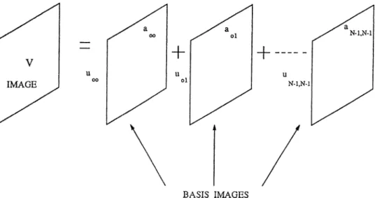
The 2-D transformations can be summarized as the representation of an image by the scaled sum of basis images. That is basis images form such a set that if they are scaled and summed properly they can construct any image. The situation can be seen in Fig.3.1. where u^j’s are the scaling coefficients.
In transform coding, we only transmit the scaling coefficients and not the image. The receiver reconstructs the original image from the basis images by
CHAPTER 3. REVIEW OF SOME WAVEFORM CODING METHODS
19
only using the scaling coefficients. By storing (or transmitting) the relatively large scaling coefficients, in magnitude, of the basis images we can remove the redundancies in the original image. For instance, a very small coefficient in magnitude implies a very small information for that specific basis image. Hence, we usually drop or give less emphasis to such coefficients in coding. In this way, we improve our compression results without much distorting the visual quality.
A transformation should have the ability to represent an image by as less scaling coefficients as possible^ In image coding Discrete Cosine Transform is the most popularly used transform which is described ne.xt.
Discrete Cosine Transform
The NxN discrete cosine transform F{ u, v) of an image f { j , k) is defined as
A ^ - l N - l F{ u, v) = i C{ u) C{ v) Y f { j , k) . cos j=0 k=0 {2j + l)u7r 2N . cos (2k + l)u7T 2N for u, u = 0,1, · ■ ·, — 1 where , , I f o i ' w=0 C(w) = ^ 1 for w = l,2 ,...,N -l (3.9) (3.10)
The inverse transform is given by
N - l N - l f ( j , k ) = Y ^ Y ^ C ( u ) C { v ) F ( u , v ) . c o s u=0 v=0 for = 0,1, · · ·, — 1. (2j -f- l)ri7T nr\ Q (2k -f l)v'K 2N . CUo 2N (3.11)
DCT is a separable transform and it has very high energy compaction prop erty for images with high correlations among neighboring pixels [7].
As it is well known Karhaunen-Loeve transform (KLT) is the optimum transform in terms of energy compaction. However, KLT is dependent on the statistics of the input signal hence it has a signal dependent coefficient matrix and not very convenient forjnost practical image processing applications. D C T has a constant transform matrix (independent of the input signal statistics) so it is suboptimum however, much easier to implement. DCT is a very good
CHAPTER 3. REVIEW OF SOME WAVEFORM CODING METHODS
20
approximation to the KLT for the order highly correlated Markov sequences. An N x N D CT matrix is very close to the KLT matrix of a first order stationary Markov sequence of length N whose covariance matrix is given by
R = 1 P 9
1
P P r.N-1 r.N-2 ^N-1 „N-2 (3.12) p‘ ' ^ r ^ p 1when the correlation parameter p is close to unity [7]. Hence, it is widely accepted and even used in some image transmission standardization proposals [18]. Fast DCT algorithms can also be implemented by using FFT algorithms. DCT of a vector of N elements can be calculated in 0{Nlog2N) operations via an N-point FFT [19] which we used this property in our DCT implementations.
The adaptive DCT coder that we implemented for image compression pur poses performs transform domain coding. The algorithm is a modified version of the study by [1] and by itself a lossy coding scheme.
We first divide the image in small sub-blocks of typical size 8 x 8 pixels then take the DCT of each sub-block and put a threshold (T ) on the trans form domain coefficients. This threshold can be adjusted to eliminate sriiall amplitude coefficients which do not carry much information. The coefficients with amplitudes less than the predefined threshold (T ) are made zero, where the others are scaled by the threshold amount T. In this way the number of zero amplitude coefficients are increased and longer run-lengths are obtained^. While doing so we do not touch the luminance value of the sub-block which is the (0,0)’th coefficient of the DCT transformed sub-block because this value determines the intensity of the “blocking effect” which is easily observed vi sually (Mean values of the consecutive blocks change, if the luminance value is harshly quantized). Blocking effects occur due to the quantization of the transform domain coefficients and appears as small blocks of different intensi ties on the image. It destroys the visual quality and mean square error of the image. In order to avoid “blocking effect” we do not threshold the luminance value (this is the dominating factor in “blocking effect” ) of the transformed sub-block and quantize it to full range which is 9 bits.
Rest of the transform domain coefficients are then quantized by the user defined quantization step (.S'). While doing so we quantize the small amplitude coefficients in better precision regardless of the user defined quantization step (S). This in return preserves the visual quality of the image.
CHAPTER 3. REVIEW OF SOME WAVEFORM CODING METHODS
21
Figure 3.2: Zig-zag scan
A modified Huffman coclebook and a run-length codebook (explained in Sec tions 3.1.2,3.1.3) are then adaptively constructed according to the quantization step S.
The quantized block of coefficients are “zig-zag” scanned as seen in Fig.3.2. This zig-zag scanning structure optimizes the number of run-lengths of ze ros and end-of-blocks. (During zig-zag scanning “zero-bridging^” is also per formed). Because among many functions which model the probability density of the cosine transform coefficients F '(u,u), the Laplacian density has shown to provide the best fit [1]. This function can be written as
p{x]u,v) =
y/2<r{u,v) exp (3.13)
W/here a{u^v) denotes standard deviation of a coefficient.
After run-lengths of zeros are determined and other coefficients are zig-zag scanned a predefined range is variable length coded, and the rest is fixed length coded (detailed explanation of the coding procedure is given in Section 3.1.3).
The performance of the coder is quite good in terms of mean square error and subjective evaluations. For instance, a compression ratio of 10 can be achieved without any visual degradation (subjective measure) for some images including the well known “Lena” . Typical codebook pairs used for coding transform domain coefficients and run-lengths are given in Fig.3.3.
CHAPTER 3. REVIEW OF SOME WAVEFORM CODING METHODS
22
NUMBER OF
AMPLITUDE CODE BITS HUFFMAN CODES
-6 8 00000000 -5 8 01100000 -4 7 0000001 -3 5 01101 -2 4 0111 -1 1 1 1 3 001 2 5 00001 3 6 011001 4 7 0110001 5 8 00000001 6 8 01100001 EOB 4 0001 RL PREFIX 3 010 [ 38.-38] 2 +6 11+6 BITS [255,-255] 3+9 101+9 BITS RUN-LENGTH 1 3 o n 2 4 0101 3 4 0011 4 5 01000 5 5 10010 6 5 01001 7 5 10001 8 5 10011 9 5+9 1 00010+9 BITS 1
Figure 3.3: Huffman codebook for the DCT algorithm
3.1.2
The Huffman Coding
Let us assume that a discrete memoryless source U has a K letter alphabet ai, 02, Ojt with probabilities P (o i), P (a2) , P ( a r - ) . Each letter can be rep resented l)y a codeword from a prescribed codebook'^. Let the number of differ ent symbols in the codebook be D (which is 2 in binary case; 0 and 1) and the number of symbols in the codeword corresponding to cik be nk (i.e., if a;t=0111 then rik=4:).
The average number of symbols per source letter h is defined as follows:
K
= Y ^ P ( a t ) .n , (3.14) n
k=l
Any useful codebook must be uniquely decodable. We can intuitively argue that, if we can assign longer codewords to source letters with less probability
CHAPTER 3. REVIEW OF SOME WAVEFORM CODING METHODS
23
P(a ) k 0.3 a 0.25 a 0.25 a Codewords 0.550.1
0.1 a 0.2 0.45 1.00Figure 3.4: Optimum code assignment procedure
and the shorter codewords to source letters with high probability then we can represent our alphabet with less bits than the codebook which assigns fixed length codewords to each symbol. This is meaningful as most of the time the more probable source letters occur and since we assign shorter codewords to them, on the average we decrease the number of symbols transmitted.
In information theory, the well known concept of “source codiiig” says that [14]
n > II(U ) (3.15)
at all times, where H(U) is the entropy of the source U and given by K
II{U) = Y^P{ak)log2
k=l P (“ k)
(3.16)
That is, the minimum possible symbol assignment is lower bounded by the entropy (H) of the source. By proper code assignment we try to achieve the entropy value of the source alphabet.
The optimum code assignment for source letters can be achieved by Huff man coding. In this assignment algorithm source letters are given source sym bols beginning from the least probable two symbols, in a tree like structure. The coded two symbols and their probabilities are allied and a new source alphabet is formed. Then the same procedure, coding two least likely symbols, is applied recursively until we come up with one source letter. An example is given in Fig.3.4. A nice property of the Huffman coding is that, the output codewords are prefix conditioned (instantaneous). In other words, no codeword is a prefix of another codeword. Hence, decoding can be accomplished in real time without any storage requirement.
In our compression (coding) schemes we use codebooks designed by the Huffman coding algorithm. But sometimes the number symbols increase so
CHAPTER 3. REVIEW OF SOME WAVEFORM CODING METHODS
24
-6 -5 -4 -3 •2 •1 1 2 3 4 5 6 БОВ RLPREHX i 3β,-38] [255,-255] RUN-LENOTH NUMBER OF CODEBITS > 8 7 5 4 1 3 5 6 7 8 8 4 3 2 Ji-9 4 5 5 5 5 5 5^·9 HUFFMAN CODES 00000000 01100000 0000001 01101 0111 1 001 00001 011001 0110001 OCOOOOOl 01100001 0001 010 11-6 BITS 10Ь9 BITS on 0101 ООП 01000 10010 01001 10001 icon OC010f9BITS NUMBER OFAMPLITUDE CODE BITS HUFFMAN CODES
116.-1« 1+5 1+5 BITS P55,-255] 2+9 01+9 BITS RL PREFIX 3 000 EOB 3 001 RUN-LENGTH 1 2 00 2 2 10 3 4 1100 4 4 1101 5 5 11100 6 5 1Г101 7 5 11110 8 5 mil 9 2t9 01+9 вгге
Figure 3.5: Modified Huffman codebook pair
much that instead of paying the cost of a very long and complicated Huffman codebook, we pay the price of a little worse compression by making use of a modified Huffman codebook. This time, source letters within the predefined range (especially the high probable ones) are variable length coded and the remaining source letters are fixed length coded. This modification does not degrade the compression ratios (equivalently average bit per source letter) more than 5% in most cases [8]. Two such modified codebooks which we also used in our compression schemes is shown in Fig.3.5.
3.1.3
Run-length Coding
If a certain source symbol occurs consecutivel}^ in a sequence of symbols, then it is more efficient to encode this repeated symbol sequence in one codeword. For instance in a binary image sequence like facsimile, there is a great potential for intraframe redundancy reduction by means of a subsequent operation called riin-length coding. In a text the binary symbol 0 (1) representing black (white) occurs with long runs so that consecutive runs of zeros or ones can be coded.
In gray-level images (2-D sequences) although there are more than 2 levels, in smooth regions we expect to have runs of pixels. Especially, in medical im ages there are frequent runs of constant gray-level values which can be encoded by run-length coding.
CHAPTER 3. REVIEW OF SOME WAVEFORM CODING METHODS
25
Run-length coding must be an essential part of any compression unit since it is very effective in reducing the primary redundancies (Other methods such as transform coding, subband coding is necessary to reduce secondary redun dancies). A simple but popular gray-level lossless image coding is the shift and subtract scheme, in which we shift the image by one pixel to the right or left and subtract from itself to make use of repetitions in different gray-level values [20]. In this way, neighboring pixels with the same gray-level value subtract to zero and we obtain a new sequence with frequent runs of zeros®.
If “zero” valued samples are repeated consecutively then they can be en coded together by means of run-length coding. For this purpose we can reserve a special prefix called the run-length prefix and encode the number of repeti tions of zero valued samples by either fixed length or variable length codes. The receiver recognizes run-length prefix and decodes the codeword attached to it as the number of repetitions of zeros.
Run-length coding is very convenient in eliminating the redundancies in smoothly varying images. Medical images are smoother than the typical images of natural scenes. Because of this higher compression ratios can be achieved in medical image coding than the coding of natural scenes.
We can further improve the results by the concept of end-of-block (EOB) and zero-bridging (ZB).
EOB is a reserved codeword to indicate that runs of zeros continues till the end of encoded block. This saves lots of bits especially in DOT coding which will be explained in Chapter 4.
ZB can also be used if we perform lossy coding. The aim is to smooth out the isolated variations in the gray-level values and increase the number of run- lengths and E O B ’s. In zero-bridging, an isolated non-zero sample in between two zero valued samples is bridged over and converted to zero. In this way, we increase the number of run-lengths with the cost of loosing some information which can not be recovered forever.
®Note that by subtracting the image from itself we increase the range o f encoding from 8 bits to 9 bits
Chapter 4
Lossless Multirate Image Coding
4.1
Introduction to Subband Coding
In this chapter, we present our lossless multiresolution medical image coding methods. In Chapters 2 and 3 we summarized background material which is necessary for our lossless coding schemes.
In subband decomposition, either rectangular or non-rectangular^ most óf the information is localized in the low frequency range which is denoted by LL in Figs.2.7,2.9. This is due to the natural characteristics of the ordinary images. Especially, for medical images which have very little high frequency contents, the sub-images Lli, HL, HU, H contain very little information.
LL sub-image is a lower resolution version of the original image. In typical images including medical images, this sub-image contains most of the infor mation content of the original image. The rest of the sub-images carry detail information and by themselves do not even clearly represent the original image.
In order to obtain a good compression ratio, the low frequency portion sub image (LL) of the original image should be encoded very efficiently. A good compression in this range effects the overall compression ratio significantly.
In many subband coding schemes, because of the importance of the LL sub-image, DCT based compression schemes are applied and usually no visual degradation is introduced to the LL sub-image. In detail images LH, HL, HH, H where there is less information than LL other techniques such as PCM with run-length coding which are computationally less costly, are used.
In the following Sections 4.1.1. 4.1.2, 4.1.3 the coding of three sample images
26
CHAPTER 4. LOSSLESS MULTIRATE IMAGE CODING
27
N U M B E R O F A M P L IT U D E C O D E B IT S H L W M A N C O D E S [1 .4 ] 1 + 2 1 + 2 B IT S [0 .1 2 8 ] 2 + 7 0 1+ 7 B IT S R L P R E F IX 3 0 0 0 E O B 3 001 R U N -L E N G T H 1 2 00 2 2 10 3 4 1100 4 4 1101 5 5 111 00 6 5 l l l O l 7 5 11110 8 5 11111 9 2+ 9 0 1+ 9 B r r sFigure 4.1: Codebook for low information sub-images
with different methods is explained. The “Lena” image, although it is not a medical image, is used to compcire our results with the ones reported in the survey of M. Rabbani and P.W. Meln^mhuck [8].
4.1.1
Coding with nonrectangular
subband decomposition
In nonrectangular decomposition the image is split into 3 sub-images via di amond shaped filters (The decomposition procedure and the filters used are explained in detail in Section 2.1.1). These 3 images are referred as LL, LH and H ( see Fig.2.7 ). The rest of the work is to apply appropriate coding to each of these sub-images.
The sub-images LH and H contain very low information and full of zero valued samples. So we can reach very high compression ratios (in the order of lO’s) by run-length coding of these sub-images. As usual the sub-images LH, H do not carry much information and dominated with zero samples. Hence, we can very efficiently compress them by run-length coding the zero samples and variable length coding the non-zero samples.
A specially designed run-length codebook suitable for these sub-images (LH and H) is used. The codebook which we used is shown in Fig.4.1. In order to reduce the complexity of the coder without drastically decreasing the com pression ratio, we applied the modified Huffman code book design technique which was explained in Section 3.1.2.
CHAPTER 4. LOSSLESS MULTIRATE IMAGE CODING
28
Figure 4.2: DCT coding structure
In our modified Huffman codebook we divided the source symbols into four main categories
1) The zero valued samples till the end of block which are encoded by FOB code;
2) Consecutive zero valued samples which are encoded by variable length codes after the run-length prefix (RL-pre);
3) Samples with low amplitudes which are encoded by fixed length codes after the low amplitude prefix; and
4) Samples with high amplitudes which are encoded by fixed length codes after the high amplitude prefix.
The assignment of these prefixes are made according to the frequency of occurance of such samples. That is, if low amplitude samples are the most probable ones then we assign short prefix to this range and etc.
The sub-image LL is encoded by two different algorithms. These algorithms are “DCT based coding” and “difference coding” .
D C T based c o d in g o f LL su b -im a g e: Commonly used DCT based coding schemes are lossy methods due to the quantization performed in the transform domain.
CHAPTER 4. LOSSLESS MULTIRATE IMAGE CODING
29
Lena 512x512 Angio 512x512 Chest 1024x1024 HL 2.82 3.61 6 . 1 1 H 3.01 3.97 4.53 DCT 5.28 4.67 17.56 Error 1.49 1.87 1.71 R 2.13 2.61 3.21 H 2.82 3.46 5.04Table 4.1: DCT based results for nonrectangular decomposition
By retaining the error image, the difference between the original and the DCT coded images, the coding scheme becomes lossless and in this way the information loss introduced by DCT compression is compensated. The overall bits used to encode LL is the sum of the bits used for the encoding of “error image” and the “DCT coding” . However, because of the high quality com pression of the DCT the “error image” do not carry much information and dominated with consecutive zero samples so it is run-length coded as in the case of LPI and H sub-images.
At this point, we should note that DCT compression is an adaptive scheme and can compress the same image to varying ratios by the change of
user-dependent inputs such as the threshold (T ) and the quantization step (5 ). This change also effects the “error image” statistics, as the information loss due to DCT compression depends on the constants T amd S. Hence, an optimum point between DCT compression and “error image” compression can be found.
We performed many experiments with the structure of Fig.4.2 using the codebook of Fig.4.1 for sub-images LH, H and obtained results which are pre sented in Table 4.1.
In the table R value is the realized total compression ratio and the H is the theoretical entropy value'. PIL, H are realized compression ratios for subbands HL and H respectively. DCT and Error cue the realized compression ratios for the DCT algorithm and error image respectively, for sub-image LL.
D iffe r e n ce c o d in g o f LL su b -im a g e: This method is easier to implement than the DCT based method for coding the LL sub-image. This can be the shift and subtract method which was mentioned in Section 3.1.3. This time LL sub-image is shifted by one pixel to the right cuid subtracted from itself, and resulting difference image is variable length and run-length coded. The results of the shift and subtract ojoeration is presented under LL column. In this way we achieve the results of Table 4.2.
^One should note that the values in Tables 4.1-4.5 are the compression ratios not the average bits and the results of the DCT algorithm is obtained with codebook of Fig..3.3
CHAPTER 4. LOSSLESS MULTIRATE IMAGE CODING
30
Lena 512x512 Angio 512x512 Chest 1024x1024 LL1.20
1.55 1.48 HL 2.82 3.61 6 . 1 1 H 3.01 3.97 4.53 R 2.16 2.81 3.10 H 2.53 3.25 4.50Table 4.2: Difference based results for nonrecrangular decomposition
We obtained similar results for all the medical images we tried although there may be images where these two methods differ a lot from each other. The difference coding is faster and easier to implement than the DCT based coding besides there is no need to code the “error image” as the method is lossless from the start. However, DCT corni^ression achieves very high compression ratios in the case of lossy coding (with out considering the “error image” ), and in situations whei'e some loss can be tolerable it is superior to any other method.
4.1.2
Coding with rectangular subband decomposition
The coding scheme with rectangular decomposition is very similar to the “cod ing with nonrectangular decomposition” which was explained in the previous section. This time decomposition of the image into lower resolutions is done by rectangular exact reconstruction filters described in Section 2.1.1 and the image is split into four sub-images which will be referred as LL,LH,HL and HH (see Fig.2.9).
As usual the sub-images LH, HL, HH do not carry much information and dominated with zero samples. Hence, we can very efficiently compress them by run-length coding the zero samples and variable length coding the non-zero samples using a similar codebook of the previous coding scheme^.
The problem of coding the LL sub-image is handled as in the case of pre vious section. To code the LL sub-image we again use the same methods that we used in Section 4.1.1: DCT based coding and Difference coding .
D C T based c o d in g o f LL su b -im a g e: We code the LL sub-image by using the lossy DCT algorithm and compensate the information loss by the “error image” as in Section 4.1.1. The encoder extracts the “error image” by the structure defined in Fig.4.2. DCT coefficients are coded by the algorithm explained in Sections 4.1.1 and 3.1.1 is run length coded as usual due to low
CHAPTER 4. LOSSLESS MULTIRATE IMAGE CODING
31
LH HL HH DCT Error R H
Lena 512x512 3.40 2.69 4.69 5.27 1.50 2.30 3.10
Angio 512x512 3.83 3.75 12.86 4.70 1.85 2.94 3.89 Chest 1024x1024 4.35 8.34 62.93 17.48 1.72 3.98 6.04
Table 4.3; DCT based results for rectangular decomposition
LH HL HH LL R H
Lena 512x512 3.40 2.69 4.69 1.20 2..34 2.76 Angio 512x512 3.83 3.75 12.86 1.53 3.17 3.65 Chest 1024x1024 4.35 8.34 62.93 1.47 3.82 5.39
Table 4.4: Difference based results for rectangular decomposition
information nature of it. These two iniciges ( “DCT coded" and “error image” ) together reconstructs the original LL sub-image e.xactly. We did similar exper iments on the same images which are shown in Fig.4.4 and, 4.5 and the results presented in Table 4.3 are obtained.
The results are about 14.8% better than the results of “nonrectangular decomposition” .
D iffe re n ce c o d in g o f LL su b -im a ge: The same procedure of the Section 4.1.1 is applied, that is we shift and subtract the LL sub-image from itself and variable length and run-length code the “difference image” . The results of the performed experiments is described in Table 4.4.
We note that both in rectangular and nonrectangular subband decom po sitions the LL sub-image coding results are the same. This is due to the fact that in both cases LL is rectangularly lowpassed and downsampled version of the original image. So, the main difference between the two methods come from the coding of other sub-images such as Lli, HL etc.
4.1.3
Pyramidal Coding
Pyramidal coding is a multirate coding scheme as described in Section 2.1.2. The image a’ (n) is low pass filtered and down sampled by 21 j. to a:6(n). The 2-D low pass filter is a separable anti-aliasing filter and obtained by the mul tiplication of 1-D low pass filters as explained in Equation 2.32. The down
CHAPTER 4. LOSSLESS MULTIRATE IMAGE CODING
32
x^n)
Figure 4.3: Pyramidal coding with lossy DCT
sampling matrix is
2/ =
2 0 0 2
(4.1)
and hence the resolution of the image is reduced by 4 (|<iei(2/)| ). This in return also reduces the size of the image by 4. In other words an image a;(n) of size 512 X 512 reduces to an image a;t(n) of size 256x256 as shown in Fig.4.3.
This low resolution sub-image is very similar to the LL sub-image of the previous subband coding methods. So it carries a lot of information in many typical images. We code .Tfc(n) by the DCT algorithm. The comiaressed image is denoted by ?/6(n) in Fig.4.3. DCT coding introduces some loss to this low resolution image i/6(n). We upsample the DCT coded sub-image y6(n) by 2 / | and low pass filter it with the same filter of the down sampling block, to y(n) whose size is the same as the size of the original image. The reconstructed image y(n ) is not an exact replica of the input image a:(n) due to DCT coding and multirate signal processing operations. We obtain an “error image” .i'(n) which is the difference between the original image and the reconstructed image. The “error image” carries very little information and dominated with consecutive zero samples so, can be very effectively run-length coded. In lossy image coding the “error image” is coded by a dead-zone quantizer to increase the efficiency of the run-length coding. In our lossless coding method to achieve perfect reconstruction at the receiver we do not quantize the “error image” .
The ’’ error image” is dominated with low amplitude samples and many consecutive zeros, hence we use “modified Huffman” codebook concept for coding the nonzero samples, i.e.,Coding of the “error image” is carried out as
CHAPTER 4. LOSSLESS MULTIRATE IMAGE CODING
33
DCT Error R H
Lena 512x512 2.87 1.48 1.31 1.81
Angio 512x512 5.13 1.71 1.58 2.10 Chest 1024x1024 17.56 1.68 1.64 2.41
Table 4.5: Pyramidal compression results
Figure 4.4: The sample image “Angio”
the coding of detail images LH, HH, etc. of subband decomposition structures. The results obtained with the pyramidal coding cilgorithm are summarized in Table 4.5
Although the results are promising thej' are no better than the subband coding results. By comparing Tables 4.1-4.4 with Table 4.5 we observe that pyramid coding method is inferior to the subband decomposition structures.
CHAPTER 4. LOSSLESS MULTIRATE IMAGE CODING
34
Figure 4.5: l / 4 ’" ‘ of the sample image ‘'Chest” and “Lena”
4.2
Conclusion
Picture Archiving and Communication Systems (PACS) have recently been deployed in radiology departments. A PACS requires huge amounts of data to be stored in different storage media. The capacity of the memory of a PACS must be used as efficient as possible. The compression of medical images must be carried out in order to reduce the memory size. There are image coding methods which reduces the storage size of an image by an amount of 1/10 with out any visual degradation. But in some medical applications lossless coding of medical images is necessary. Although lossless coding can not achieve high compression ratios as lossy coding, any PACS should have the capability of storing medical images without introducing any loss.
Multiresolution coding techniques have been used for lossy image and speech coding, in this thesis we developed multiresolution techniques for the lossless image compression. We observed that the use of multiresolution techniques in lossless compression is as much advcintageous as in loss}'· compression schemes. The main application area of the new technique is the coding of medical images.
The most popular multiresolution signal representation method, subband decomposition^ plays a key role in our compression algorithms. We applied two different subband decomposition methods, rectangular and nonrectangular, in conjunction with DCT coding to compress the medical images. Although the compression schemes are adaptive and image dependent, we observe that the rectangular decomposition results are a little better than the nonrectangular decomposition.
CHAPTER 4. LOSSLESS MULTIRATE IMAGE CODING
35
The results presented in Tables 1 to 4 in Chapter 4 are about 6.3% superior than the ones recorded in the work of M. Rabbani and P.W. Melnychuck [8]. The well known image “Lena 512x512” is used to compare our results with the previous studies of the same work reported in the survey of [8]. For this specific image the best result is obtained in the difference coding of the rectangular decomposition in Table 4 which is 11.4% better than the best result of [8].
Another popular multiresolution method “pyramidal decomposition” is also considered. The results of Table 5 are inferior to the subband coding based methods (Tables 1 to 4). This is due to the fact that pyramidal decomposi tion produces more samples than the number of samples of the image at each decomposition stage.
The results presented in this thesis are obtained with fixed code books of Fig.3.5 and 4.1 and can be improved about 5% by use of an adaptive code book. But adaptive code book assignment has the disadvantage of extra information for decoding at the receiver.
Arithmetic coding of LH, HL, HH and H sub-images can be considered to improve the results because arithmetic coding can produce results which arbitrarily closely approach the entropy value .
The algorithms proposed in this thesis can easily be extended to the 3-D compression of medical images by only adding an extra motion detection algo rithm.