Compact optical temporal processors
David Mendlovic, Oded Melamed, and Haldun M. Ozaktas
Optical signal processing can be done with time-lens devices. A temporal processor based on chirp-z transformers is suggested. This configuration is more compact than a conventional 4-f temporal processor. On the basis of implementation aspects of such a temporal processor, we did a performance analysis. This analysis leads to the conclusion that an ultrafast optical temporal processor can be implemented.
1. Introduction
A signal processor is the main component of many digital or analog computers. The computing rate of the processor may determine the speed of the whole system. Recently, several optical systems were sug-gested1–3that can achieve ultrafast serial processing by employment of the analogy between optical spatial diffraction and temporal dispersion.4–6 In the follow-ing, a temporal processor that is based on a chirp-z transformer is suggested. As the first step toward practical implementation of the suggested system, its performance analysis was done. This analysis takes into account the state-of-the-art option for the time-lens device. In Section 2, for the sake of notation, the relevant background is briefly presented.
2. Optical Temporal Processor Based on Time Lenses
In this section we summarize basic concepts in the theory of optical temporal processing based on time-lenses. A detailed description of this theory is given in Ref. 2.
A monochromatic field distribution u1x, z 5 02 with spatial spectrum U1µ2 that travels along the z axis will experience spatial diffraction according to Fresnel theorem:
u1x, z $ 02 . C exp1ikz2
e
U1µ2exp12iplzµ223 exp1i2pµx2dµ. 112
The term exp12iplzµ22 is known as the spatial disper-sion term. C is a complex constant.
A temporal signal u1t, z 5 02 with a spectrum U1v2 that travels along the z axis of a dispersive delay line will accumulate phase delay
exp5i2p3vt 2 b1v2z46, 122 where v is the temporal analog of µ and b1v2 is commonly approximated as
b1v2 < b01 b1v 1 b21v2@22. 132 b1is the group velocity of the propagated wave and b2 is the quadratic dispersion term. If we neglect irrel-evant factors, the propagated signal from z 5 0 to z is
u1t, z2 5
e
2``
U1v2exp12ipb2zv22exp3i2pv1t 2 b1z24dv. 142 Comparison of approximation 112 and Eq. 142 leads to the similarity between the spatial dispersion term exp12iplzµ22 and the temporal dispersion factor exp12ipb2zv22. This similarity is the basic motiva-tion for developing such optical temporal processors. For the general convolution processor the temporal analogs for the spatial 2-f and 4-f systems were designed.2 The basic components of these spatial systems 1Fig. 12 are 112 free-space propagation, 122 spatial lenses, and 132 spatial filters. According to the above duality, one can define the appropriate components of the temporal 2-f and 4-f processors: 112 dispersive delay lines, 122 time-lenses,6,7 and 132 temporal filters.
Figure 2 shows a schematic 2-f system that per-forms the temporal Fourier-transform operation. It consists of propagation in a dispersive line along a length f, passage through a time lens, and again D. Mendlovic and O. Melamed are with the Faculty of
Engineer-ing, Tel Aviv University, Tel Aviv 69978, Israel. H. M. Ozaktas is with Department of Electrical Engineering, Bilkent University, Bilkent 06533, Ankara, Turkey.
Received 7 July 1994; revised manuscript received 18 January 1995.
0003-6935@95@204113-06$06.00@0. r1995 Optical Society of America.
propagation in another dispersive line along a length
f. The time lens is described by the phase factor
L1t2 5 exp
3
2ip1
t 2 t1 t2
2
4
, 152where t and t1 are the time-lens parameters that control the lens performance.2 t relates to the focal length, and t1relates to the lateral location of the lens in the spatial analog system. It was shown2that for achieving the 2-f system, t and t1 should satisfy the following equations:
t25 b
2f, 162
t15 b1f 172
A time lens can be implemented either as an electro-optic phase modulator7,8or as an electro-optic ampli-tude modulator driven by an electrical chirp signal.
If the input signal at z 5 0 is u01t2 5 u1t, 02, the output signal of the 2-f temporal processor2is
u1t, 2f 25 U0
1
t 2 2fb1t2
2
, 182where U01v2 is the Fourier transform of u01t2. Now let us expand the 2-f Fourier transformer to the basic Fourier-optics processor. The 4-f configuration, which contains two 2-f systems in cascade 1Fig. 32, is a 1:1 imaging setup capable of Fourier-plane filtering. The 4-f configuration includes two lenses. The first lens parameters are those that we calculated earlier for the 2-f system. The second lens2 has the same focal length as the first lens,
t25 b
2f, 192
but t1is changed to
t15 3b1f. 1102 For these parameters the output signal is
u1t, 4f 25 u014fb12 t2. 1112 It is exactly a delayed reverse 1:1 image of the input signal; i.e., the front and the end of the image are exchanged.
Implementation of such a processor requires four dispersive delay lines with length f and four electro-optic modulators: one to modulate the input signal, one for each time lens, and one for Fourier-plane filtering. In Section 3 an alternative approach is suggested that requires only three electro-optic modu-lators and two dispersive delay lines.
3. Temporal Processors Based on the Chirp-z Transformation
A. Temporal Chirp-z Transformer
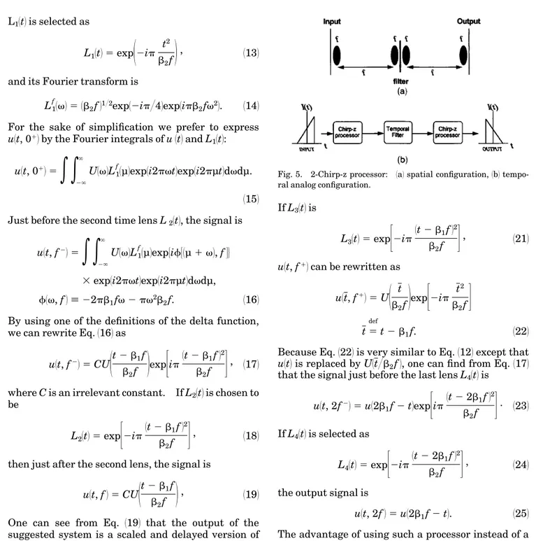
As in spatial optics, the use of chirp-z transformation could provide several benefits. Figure 41a2 shows a schematic spatial processor that performs a spatial Fourier transform. The setup is based on an optical implementation of the chirp-z transformation.9 It consists of three subsystems in cascade: transfer through a lens, free-space propagation, and again transfer through a lens. For the temporal dual case we multiply the input temporal signal with a time lens, then we let it propagate over a distance f, and finally we multiply it with another time lens3Fig. 41b24. Now let us start with an initial signal u1t2 with temporal spectrum U1v2. Just after the first time lens L11t2, the signal is
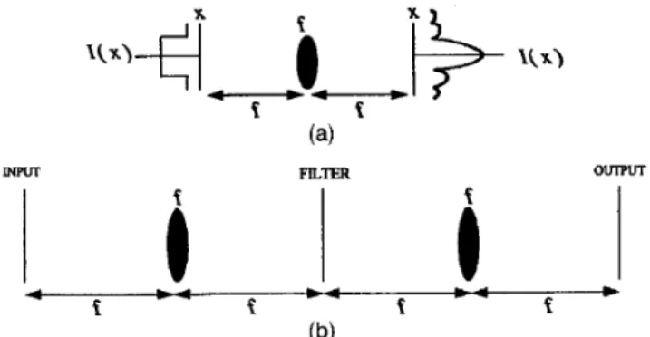
u1t, 012 5 u1t2L11t2. 1122 Fig. 1. Spatial processors: 1a2 2-f system; the output of this
system is a scaled Fourier transform of the input image. 1b2 4-f system; this is a basic Fourier optics image processor, which contains two 2-f systems in cascade. 1b2 is a 1:1 imaging setup capable of Fourier-plane filtering.
Fig. 2. Optical temporal 2-f system.
Fig. 3. Optical temporal 4-f processor.
Fig. 4. Chirp-z transformer: 1a2 spatial configuration, 1b2 tempo-ral analog configuration.
L11t2 is selected as
L11t2 5 exp
1
2ip t 2b2f
2
, 1132
and its Fourier transform is
L1
f
1v2 5 1b2f21@2exp12ip@42exp1ipb2fv22. 1142 For the sake of simplification we prefer to express
u1t, 012 by the Fourier integrals of u 1t2 and L11t2:
u1t, 012 5
e e
2``
U1v2L1f1µ2exp1i2pvt2exp1i2pµt2dvdµ. 1152 Just before the second time lens L21t2, the signal is
u1t, f22 5
e e
2` ` U1v2L1f1µ2exp5if31µ 1 v2, f 46 3 exp1i2pvt2exp1i2pµt2dvdµ, f1v, f 2 ; 22pb1fv 2 pv2b 2f. 1162By using one of the definitions of the delta function, we can rewrite Eq.1162 as
u1t, f22 5 CU
1
t 2 b1f b2f2
exp3
ip1t 2 b1f2 2 b2f4
, 1172 where C is an irrelevant constant. If L21t2 is chosen to beL21t2 5 exp
3
2ip1t 2 b1f2 2b2f
4
, 1182
then just after the second lens, the signal is
u1t, f 2 5 CU
1
t 2 b1f b2f2
, 1192
One can see from Eq. 1192 that the output of the suggested system is a scaled and delayed version of the temporal Fourier transform of the input signal.
B. Temporal Filtering System Based on Chirp-z Transformers
The spatial imaging processor that is capable of Fourier-plane filtering is shown in Fig. 51a2. The temporal analog case is depicted in Fig. 51b2. It consists of two chirp-z transformers placed in cascade. In the following this configuration is denoted as a 2-chirp-z processor. The input signal for the second transformer is expressed in Eq. 1192. Just after L3, the signal is u1t, f12 5 U
1
t 2 b1f b2f2
L31t2. 1202 If L31t2 is L31t2 5 exp3
2ip1t 2 b1f2 2 b2f4
, 1212 u1t, f12 can be rewritten as u1t, f12 5 U1
t b2f2
exp3
2ip t 2 b2f4
t 5 def t 2 b1f. 1222Because Eq.1222 is very similar to Eq. 1122 except that
u1t2 is replaced by U1t@b2f2, one can find from Eq. 1172 that the signal just before the last lens L41t2 is
u1t, 2f22 5 u12b1f 2 t2exp
3
ip1t 2 2b1f2 2 b2f4
. 1232 If L41t2 is selected as L41t2 5 exp3
2ip1t 2 2b1f2 2 b2f4
, 1242the output signal is
u1t, 2f 2 5 u12b1f 2 t2. 1252 The advantage of using such a processor instead of a conventional 4-f processor is that it can be imple-mented with only two dispersive delay lines and three electro-optic modulators: the first modulator modu-lates the input signal multiplied by the first time lens, the second implements the second and the third time lenses 3L21t2 and L31t24, and the third implements the last time lens3L41t24. In many applications, u1t2 is real and positive. In such cases the third modulator is not required, and the system can be implemented with only two electro-optic modulators.
4. Performance Analysis
A. The Chirp-z Fourier Transformer
For estimating the performance of the chirp-z tempo-ral configuration two considerations are used. The first is to prevent any noncausal information along Fig. 5. 2-Chirp-z processor: 1a2 spatial configuration, 1b2 tempo-ral analog configuration.
the signal flow. Second, overlapping between the signal and its processed version is not possible.
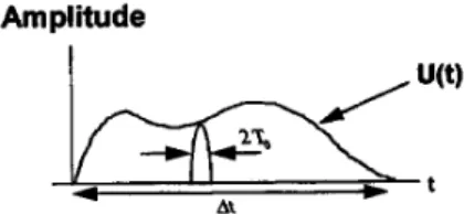
Figure 6 shows the input signal with a width of Dt and finest resolution of 1@Dv1Dv is the signal band-width2. To find the signal’s width Dt1after propaga-tion in a dispersive line with a length f, we first discuss the effect of group-velocity dispersion on a Gaussian pulse10:
s1t, z 5 02 5 exp12 t2@2T 0
22. 1262
T0is the half-width1at the 1@e intensity point2. By using Eq.142 and carrying out the integration, we can obtain the amplitude at any point z:
s1t, z2 5
1
T0 2 T022 ib2z2
1@2 exp3
2 1t 2 b1z2 2 21T022 ib2z24
. 1272The width of the Gaussian pulse increases and be-comes T15 T0
3
1 11
zb2 T022
24
1@2 . 1282If1zb2@T0222: 1, Eq.1282 can be rewritten as
T15 zb2@T0. 1292 The input signal u1t2 can be considered as composed of NPs1NPs : 12 resolution points, each with a Gauss-ian shape and half-width T0 5 2@Dv 1Fig. 72. The signal’s widening is thus 2T1, and its width just before the second lens at z 5 f2becomes
Dt15 Dt 1 b2fDv. 1302 In analogy with a spatial processor, Dt1is the required second-lens aperture, an important parameter that affects the system’s time–bandwidth-product perfor-mance. To prevent noncausal signals, we have to
assume that
Dt1, b1f, 1312
where b1f is the propagation time from the input
plane to the second lens. To prevent overlapping 1Fig. 82, we should make the time distance between two successive signals
dT . Dt1. 1322
As Eq. 1192 shows, the output signal of the chirp-z transformers is a scaled Fourier transform of the input signal. The temporal width of the output signal Dt2is thus
Dt25 b2fDv. 1332
The spectrum of the output signal can be determined from
FT3u1t, f 24 5 FT
3
U1
t 2 fb1t2
24
5 Cu12b2fv2. 1342 FT indicates the Fourier transform, and C is an irrelevant constant. The spectral width of the out-put signal isDv25 Dt@b2f. 1352
For achieving temporal filtering a temporal filter should be used in the Fourier plane. Its temporal width, DtF, and spectral width, DvF, are
DtF5 Dt2, 1362
DvF. Dt@b2f. 1372 Expressions 1302–1372 state all restrictions on the chirp-z Fourier transformer and permit the calcula-tion of the system’s performance.
Expressions1302 and 1312 can be reduced to
Dt , f1b12 b2Dv2. 1382 Because D t . 0, inequality1382 leads to the conclusion that, when a dispersive line is chosen, the following relation between the group velocity and the disper-sion term must exist
Dv , b1@b2. 1392
If DvM is the maximum bandwidth of the available
Fig. 6. Schematic illustration of the input temporal signal with a total width of Dt and a finest resolution of 1@Dv.
Fig. 7. Input signal is composed of NPs resolution points, each
modulator, and assuming that Dv 5 DvF5 DvM, Eq.
1372 can be rewritten as
Dt , DvMb2f. 1402
The system is a serial processor in first-in first-out configuration. The processor’s input are signals with a frame width of Dt that enter the system, one after another, every dT. The suggested configuration, con-sisting of a modulator with a bandwidth of DvM, can
process NPs points 1or pixels2 every signal frame, where NPsis given by
NPs5 DtDvM, 1412
The restrictions on the signal’s width Dt are given in inequalities1382 and 1402 and can be rewritten, respec-tively, as
Dt 511@c12 f 1b12 b2Dv2, c1. 1, 1422 Dt 511@d12DvMb2f, d1. 1, 1432 where c1 and d1 are constants determined by the system’s designer. The signal’s width is determined by the more limiting expression, i.e., the one that causes the frame width Dt to be smaller. Substitu-tion of Eqs.1422 and 1432 into Eq. 1412 yields
NPs5 MIN311@c12 f 1b12 b2DvM2DvM, DvM
2
b2f11@d124,
c1, d1. 1. 1442 MIN is for the minimum function that chooses the most limiting expression in the square brackets.
Because the system processes 1@dT frames every second, the total number of processed points per second is determined by
N 5 DtDvM@dT. 1452
By using expressions1302 and 1322, we can write dT as a function of the signal’s width Dt:
dT . Dt 1 b2fDvM. 1462
If the restrictions imposed on Dt3Eqs. 1422 and 14324 are substituted into inequality 1462, then this inequality can be rewritten as
dT 5 c2311@c12 f 1b12 b2DvM2 1 fb2DvM4, c2. 1,
1472 or
dT 5 d2311@d12 fb2DvM1 fb2DvM4, d2.1. 1482
Equations1472 and 1482 are related to the restrictions expressed in Eqs.1422 and 1432, respectively. c2and d2 are constants that are chosen by the system’s de-signer and actually replace the inequality sign in inequality1462. Therefore the total number of points processed by the system every second, N, can be
calculated by N 5 MIN
5
1b12 b2DvM2DvM c23b11 b2DvM1c12 124 , DvM d21d11 126
, c1, c2, d1, d2. 1. 1492 In conclusion of this section, Eq. 1492 shows that proper design of the system can accelerate the process up to a rate of DvM@2 points per second.B. 2-Chirp-z Processor
The 2-chirp-z processor can be separated into two chirp-z subsystems in cascade. The first chirp-z Fou-rier transformer was analyzed in Subsection 4.A. The second Fourier transformer is analyzed similarly but with different input parameters. The input sig-nal is
u1t, 2f 2 5 U
1
t 2 2fb1 b2f2
, 1502
and its temporal and spectral widths, respectively, are
Dt25 b2fDv, 1512
Dv25 Dt@b2f. 1522
The analysis of the whole system leads to the conclu-sion that no further restrictions are added by the second transformer, and thus the number of processed points per second is identical whether the system consists of one or two chirp-z transformers.
C. Typical Example
In this subsection we discuss a typical example of a temporal processor with a time lens. The input signal and the time lens are created with an electro-optic modulator. Present technology offers modula-tors with DvM5 30 GHz. A dispersive delay line is
used with b25 4.5 3 10220s2@m, b
15 5 3 1029s@m, and f 5 50 m. Such dispersion can be achieved in optical fiber filters.11 The input width is chosen to be Dt 5 3.4 3 1028s, and the time distance between two successive signals is dT 5 2 3 1027s. According to Eq.1412, this system can process approximately 1020 points per session and a total of 5 3 106sessions per second.
5. Conclusions
An optical temporal filtering processor based on chirp-z transformers has been analyzed. Because the implementation of optical processors based on a time lens is very complicated and expensive, there is a great importance in reducing the number of compo-nents of the system. The suggested system is more compact than a conventional 4-f setup because it requires only two dispersive delay lines with a length
f and three electro-optics modulators at most. A performance analysis was done to motivate further research in implementing the suggested system.
References
1. A. W. Lohmann and D. Mendlovic, ‘‘Temporal perfect-shuffle optical processor,’’ Opt. Lett. 17, 882–884119922.
2. A. W. Lohmann and D. Mendlovic, ‘‘Temporal filtering with time lenses,’’ Appl. Opt. 31, 6212–6219119922.
3. T. Mazurenko, ‘‘Time-domain Fourier-transform holography and possible applications in signal processing,’’ Opt. Eng. 31, 739–749119922.
4. S. A. Akhmanov, A. S. Chirkin, K. N. Drabovich, A. I. Kovrigin, R. V. Khokhlov, and A. P. Sukhorukov, ‘‘Nonstationary nonlin-ear optical effects and ultrafast light pulse formation,’’ IEEE J. Quantum Electron. QE-4, 598–605119682.
5. A. Papoulis, ‘‘Pulse compression, fiber communication, and
diffraction: a unified approach,’’ J. Opt. Soc. Am. A 11, 3–13 119942.
6. B. H. Kolner, ‘‘Space–time duality and the theory of temporal imaging,’’ IEEE J. Quantum Electron. 30, 1951–1963119942. 7. B. H. Kolner and M. Nazarathy, ‘‘Temporal imaging with a
time lens,’’ Opt. Lett. 14, 630–632119892.
8. B. H. Kolner, ‘‘Active pulse compression using an integrated electro-optic phase modulator,’’ Appl. Phys. Lett. 52, 1122– 1124119882.
9. A. VanderLugt, Optical Signal Processing1Wiley, New York, 19922.
10. G. P. Agrawal, Nonlinear Fiber Optics1Academic, New York, 19892, Chap. 3.
11. H. G. Winful, ‘‘Pulse compression in optical fiber filters,’’ Appl. Phys. Lett. 46, 527–529119852.