AN EMPIRICAL ANALYSIS OF EFFICIENCY AND PRODUCTIVITY CHANGE IN THE GLOBAL AUTOMOTIVE INDUSTRY: A MALMQUIST PRODUCTIVITY INDEX APPROACH
A Master’s Thesis by ÖZLEM YAYLACI Department of Economics Bilkent University Ankara April 2009
AN EMPIRICAL ANALYSIS OF EFFICIENCY AND PRODUCTIVITY CHANGE
IN THE GLOBAL AUTOMOTIVE INDUSTRY: A MALMQUIST PRODUCTIVITY INDEX APPROACH
The Institute of Economics and Social Sciences of
Bilkent University
by
ÖZLEM YAYLACI
In Partial Fulfillment of the Requirements for the Degree of MASTER OF ARTS in THE DEPARTMENT OF ECONOMICS BİLKENT UNIVERSITY ANKARA April 2009
I certify that I have read this thesis and have found that it is fully adequate, in scope and in quality, as a thesis for the degree of Master of Arts in Economics.
--- Assoc. Prof. Fatma Taşkın Supervisor
I certify that I have read this thesis and have found that it is fully adequate, in scope and in quality, as a thesis for the degree of Master of Arts in Economics.
---
Assistant Prof. Selin Sayek Böke Examining Committee Member
I certify that I have read this thesis and have found that it is fully adequate, in scope and in quality, as a thesis for the degree of Master of Arts in Economics.
--- Prof. Dilek Önkal
Examining Committee Member
Approval of the Institute of Economics and Social Sciences
--- Prof. Dr. Erdal Erel Director
ABSTRACT
AN EMPIRICAL ANALYSIS OF EFFICIENCY AND PRODUCTIVITY CHANGE
IN THE GLOBAL AUTOMOTIVE INDUSTRY: A MALMQUIST PRODUCTIVITY INDEX APPROACH
Yaylacı, Özlem
M.S., Department of Economics Supervisor: Assoc. Prof. Fatma Taşkın
April 2009
This thesis examines productivity changes in automotive sectors of 26 industrial and developing countries over the period 1973-2002. Using data envelopment analysis, Malmquist productivity change indices are computed and decomposed into technical change and efficiency change components. The results show that productivity improvements by the industrial countries were attained through technical change while productivity gains of developing countries mainly arose from efficiency change. It is found that the performance of Turkey was similar to the average of developing countries showing a better performance in catching-up effect. Moreover, for the countries in the sample, automotive sector labor productivity changes are calculated. Comparing the labor productivity change and Malmquist change rankings of the countries, it is concluded that the best performer countries in terms of labor productivity change are also the best performers in terms of Malmquist productivity change index.
Keywords: Automotive Sector, Efficiency Change, Productivity Change, Malmquist Index
ÖZET
GLOBAL OTOMOTIV SANAYIINDE ETKINLIK VE VERIMLILIK DEGISIMI UZERINE EMPIRIK BIR ANALIZ:
MALMQUIST VERIMLILIK ENDEKSI YAKLASIMI Yaylacı, Özlem
Yüksek Lisans, İktisat Bölümü Tez Danışmanı: Doç. Dr. Fatma Taşkın
Nisan 2009
Bu tez, sanayileşmiş ve gelişmekte olan 26 ülkenin otomotiv sektörlerinde 1973-2002 periyodundaki verimlilik değişimlerini incelemektedir. Veri zarflama analizi kullanılarak Malmquist verimlilik değişim endeksleri hesaplanmiş, teknik değişim ve etkinlik değişimi bileşenlerine ayrılmıştır. Sonuçlar göstermektedir ki, gelişmekte olan ülkelerdeki verimlilik kazanımları büyük ölçüde etkinlik değişiminden kaynaklanırken sanayileşmis ülkelerdeki verimlilik gelişmeleri teknik değişim yoluyla kazanılmıştır. Türkiye’nin, gelişmekte olan ülkelerin ortalama performansına benzer olarak, yakalama etkisinde daha iyi bir performans gösterdiği bulunmuştur. Ayrica, örneklemdeki ülkeler için, otomotiv sektörü işci verimlilik değişimleri hesaplanmıştır. Ülkelerin işçi verimlilik değişim ve Malmquist değişim sıralamaları karşılaştırıldığında işçi verimlilik değişiminde en iyi performansi gösteren ülkelerin aynı zamanda Malmquist verimlilik değişimi endeksinde de en iyi performansi gösterdikleri sonucuna varılmıştır.
Anahtar Kelimeler: Otomotiv Sektörü, Etkinlik Değişimi, Verimlilik Değişimi, Malmquist Endeksi
ACKNOWLEDGMENTS
I would like to express my sincere gratitude to my supervisor, Assoc. Prof. Fatma Taşkın for her excellent guidance, encouragement, and patience through the development of this thesis.
I am very grateful to Prof. Dilek Önkal and Asst. Prof. Selin Sayek Böke for their valuable comments and advices.
I am very thankful to my dear friends Vesile Kutlu and Ilay Kurt for their support during the process of this thesis.
Finally, I would like to express my deepest thanks to my family for their encouragement during my studies, and I would like to dedicate this thesis to my family.
TABLE OF CONTENTS ABSTRACT………...………...……….. iii ÖZET………...………...……... iv ACKNOWLEDGEMENTS………...……...………... v TABLE OF CONTENTS………..……….……... vi CHAPTER I: INTRODUCTION....………..…... 1
CHAPTER II: AUTOMOTIVE SECTOR... 5
2.1 Contributions to Manufacturing Production……….……... 6
2.2 Contributions to Manufacturing Employment………….…...…. 11
2.3 Contributions to Manufacturing Exports………...………. 13
CHAPTER III: LITERATURE REVIEW………….……….……... 18
3.1 Productivity Literature……….…...… 18
3.2 TFP Literature……..……….….……... 22
3.3 Applications of Malmquist Index ... 23
3.4 Literature on Automotive Sector Productivity……….…...…… 26
CHAPTER IV: METHODOLOGY……….…...….. 30
CHAPTER V: DATA ... 37
CHAPTER VI: EMPIRICAL RESULTS……….………... 42
6.1 Malmquist Index and Components……….…...……… 42
6.2 Comparisons with Labor Productivity Change….….…...……. 63
6.3 Turkey……….. ……….……...……. 68
CHAPTER VII: CONCLUSION……….………...….. 71
APPENDICES
A. SECTORAL SHARES IN TOTAL MANUFACTURING... 76 B. DATA DEFINITIONS ... 92 C. RESULTS IN DETAIL... 95
CHAPTER I
INTRODUCTION
An increase in productivity results with improvements in service and quality, decrements in production cost and increments in profit and market share. Hence, productivity measurement is the major tool of monitoring the performance of a firm, a country or an industry. Understanding the productivity changes of a sector can help countries determine where they can improve their performances, which can not be seen by revenue and profit reports since these reports only show the end of production results and not the performance in the process of production. So, if countries can understand the reasons behind productivity changes, they can find ways to improve their productivity.
Automotive manufacturing sector is one of the major industries in many countries, both in terms of the total value of production, and in terms of international trade and its contributions to the economies, with its backward and forward linkages. The severe international competition among the major producers is now coupled with the increasing globalization of the production process, including more developing countries in the production chain.
In this important sector, a performance analysis is necessary to identify the changes in the relative positions of producers and underlying factors that lead to these changes. Although considerable empirical work has already been undertaken with respect to the individual country or region specific automotive sector productivity analysis, we do not know any empirical work on cross country comparisons in the global automotive sector productivity. So the motivation for this study occurs from the need to find the productivity change differences in automotive industries of industrial and developing countries in the world.
The purpose of this study is, using non-parametric linear programming techniques, to examine and compare the productivity changes among the automotive industries of 26 countries which include industrial and developing countries. Our main interests can be summarized as follows:
(1) What are the sources of change in automotive sector productivity for industrial and developing country groups? Is it due to the development of better techniques of production, which is referred as technical change or is it due to the better use of factor of production mix, referred to efficiency change?
(2) Are there significant differences between automotive sector productivity patterns of industrial countries and developing countries?
(3) Do the best performer countries in terms of productivity changes show significant variations through the years or does their productivity performance always stay the same?
(4) Can we see the effects of changes occurring in production and export patterns of developing countries in their productivity performances?
(5) Does the Malmquist Productivity Change Index, a total factor productivity measure that takes the best use of all factors of production into consideration, provide additional insights to the conclusions derived from the partial productivity change measures such as labor productivity? The automotive producers’ performance will be evaluated according to these two alternative measures of productivity.
(6) What is the main source of Turkish automotive sector productivity change and how does Turkey compare to the countries included into the sample in terms of its productivity changes in this sector?
Employing Malmquist Productivity Change Index, productivity growth is decomposed into efficiency change and technical change, namely ‘catching up’ and ‘innovation’ components, respectively. Hence, Malmquist index distinguishes explicitly between the sources of growth (either from efficiency change or technical change), so it is superior to alternative indices of TFP growth. Moreover, Malmquist index computation does not require any information on input-output prices since it is based only on quantity data, and does not require an underlying functional form specification about technology, all of which justify our use of this index as the methodology of computing productivity changes.
Using Malmquist index, we compare each country in the sample to a world production frontier of automotive sector constructed from the data defined at the three-digit level of the International Standard Industrial Classification (ISIC), a data set that includes sector level information on individual country productions. Our findings show that the productivity gains of developing
countries are largely attributable to efficiency change, and productivity improvements of industrial countries mainly arise from technical change.
This paper is organized as follows; in Chapter 2 we describe the structure of the automotive sector with a special emphasis on Turkish automotive sector. Chapter 3 presents a literature review on the methodology used to calculate the productivity changes, and Chapter 4 explains the theoretical framework supporting the model used. We present the data source and the output and input specifications in Chapter 5. Chapter 6 reports and interprets the empirical results, and finally Chapter 7 gives suggestions for future research and concludes.
CHAPTER II
AUTOMOTIVE SECTOR
The automotive sector, defined as motor vehicles, parts, and accessories , is one of the most important sectors for the world economy in terms of its effects on the economic growth of countries. The industry fosters GDP growth, provides employment and increases export values in the manufacturing sector. With all these and many other effects on the economy, the sector is a major contributor to the economic welfare of countries. Traditionally, being a producer in the automotive sector is perceived as an indicator of economic development for most countries.
The sector is also a major contributor to world production. According to the International Organization of Motor Vehicle Manufacturers, OICA, if it had been a country, its total production would be equivalent to the world’s sixth largest economy. To understand the importance of the automotive sector to the global economy, it is helpful to look at its relative position with respect to other sectors. For this purpose, we calculated the sectoral production, employment, and export shares of total world manufacturing using data from the United Nations Industrial Development Organization (UNIDO). Although this is the
data set covering the most up-to-date information about sectoral production, employment, and export patterns, it is very difficult to find comparable cross- country sector level production data for all countries; for some countries and some sectors, data are not available.
After eliminating four sectors in the dataset1 for which data are not available for the majority of the countries, and choosing countries according to the availability of data, we compared 24 sectors and 26 countries with respect to their production, employment, and export shares in total manufacturing. Since 1981 is the earliest and 2000 is the latest year for which data are available at a three-digit ISIC sector level, we present our analyses for the years 1981, 1990, and 2000, to give an idea of the evolution of the sector through the years.
2.1. Contributions to Manufacturing Production
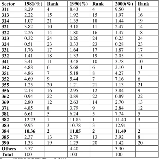
The importance of automotive sector production can be assessed by looking at the production shares of all industries in total manufacturing sector production. Shares are computed by comparing the value added generated by each sector and are reported in Table 1. In our analyses, the automotive sector is represented by the “Transport Equipment” sector (sector code: 384) since the majority of transport equipment data covers automotive-related manufacturing. The names of other sectors with their ISIC codes are presented in the Appendix A.
1
We eliminated “Petroleum Refineries”, “Misc. Petroleum and Coal Products”, “Pottery, China, Earthenware” and “Non-Ferrous Metals” sectors which are represented by the ISIC codes 353, 354, 361, and 372, respectively. Values of these sectors, whenever available, are included under the sector name of “Others.”
Table 1: Sectoral Production Shares in Total Manufacturing
Sector 1981(%) Rank 1990(%) Rank 2000(%) Rank
311 8.29 4 8.43 4 9.50 4 313 2.22 15 1.92 15 1.97 16 314 1.07 21 1.35 18 1.44 19 321 3.82 10 3.18 11 2.47 14 322 2.26 14 1.80 16 1.47 18 323 0.32 24 0.26 24 0.25 24 324 0.51 23 0.33 23 0.28 23 331 1.76 17 1.64 17 1.87 17 332 1.41 18 1.33 19 2.05 15 341 3.41 11 3.48 10 3.78 10 342 4.88 6 5.68 6 3.10 11 351 4.86 7 5.18 8 4.27 7 352 4.69 9 5.44 7 7.16 6 355 1.25 20 1.21 21 1.13 21 356 2.13 16 2.95 12 3.84 9 362 0.94 22 0.89 22 0.89 22 369 2.80 12 2.63 14 2.70 13 371 4.85 8 3.79 9 2.84 12 381 6.61 5 6.24 5 7.74 5 382 12.23 1 11.85 1 11.40 3 383 9.95 3 10.78 3 12.91 1 384 10.36 2 11.05 2 11.49 2 385 2.37 13 2.79 13 3.92 8 390 1.33 19 1.25 20 1.42 20 Others 5.57 4.40 3.30 Total 100 100 100
Source: UNIDO INDSTAT3 rev.2, 2006.
Figures indicate that in 1981, the automotive sector had a share of 10.36% of total manufacturing production and in 1990, its share increased to 11.05%. With this share, the automotive industry is ranked as the second largest sector following “Machinery, Except Electrical” in both years. In 2000, the share reached 11.49% of total manufacturing production2. All through the period
from 1981 to 2002, the automotive sector is ranked as the second largest in total
2
Since data are not available for Western Germany, Greece, Netherlands, Zimbabwe, Denmark, and Venezuela in year 2000, total manufacturing figures are calculated using the data of remaining 20 countries in that year.
manufacturing production with an increasing share. This emphasizes the growing importance of the automotive sector in manufacturing production.
If we examine countries individually, for more than half of them, the share earned by the automotive sector is ranked within the top five largest sectors in total manufacturing production in 20003. This rank was even higher for Japan, USA, the UK, France and Spain, which are the countries traditionally dominating the sector with higher production and export levels. Their automotive sectors are in the top three of manufacturing production for 2000.
In the case of Turkey, the automotive sector is ranked as the fifth largest in 1981, with a share of 4.7% of total manufacturing production. In 1990, the sector is ranked as third, increasing its share to 6%. In 2000, after “Food Products” the automotive sector is ranked as the second largest with a share of 8.4% of total manufacturing production. This illustrates the significance of the sector for Turkey’s production.
To give a better understanding of the structure of the sector, we examine the leading producers in the sector. Table 2 shows shares of countries and country groups4 in world automotive production for the years 1981, 1990, and 2000, sorted from largest to smallest share in 2000.
3 Country production shares and rankings of the sectors in total manufacturing for the years
1981, 1990, and 2000 are presented in tables 1, 2, and 3 of Appendix A, respectively.
4
Following the International Monetary Fund (IMF) World Economic Outlook, May 1993, we divided countries into industrial and developing country groups. Poland is considered a developing country although it is classified in the “countries in transition” group in the report.
Table 2: Country Shares in World Automotive Production COUNTRY 1981 (%) 1990 (%) 2000 (%) USA 39.88 34.53 40.34 JAPAN 16.89 21.43 19.25 GERMANY5 13.19 15.11 14.21 FRANCE 6.94 6.41 4.32 UK 7.16 6.49 4.16 CANADA 3.00 3.16 4.05 ITALY 4.14 3.26 2.02 SPAIN 1.64 2.31 1.58 SWEDEN 1.50 1.44 1.02 NETHERLANDS 0.60 0.55 0.49 NORWAY 0.41 0.23 0.40 AUSTRIA 0.28 0.37 0.38 PORTUGAL 0.14 0.13 0.20 DENMARK 0.27 0.25 0.14 GREECE 0.21 0.10 0.12 FINLAND 0.36 0.31 0.11 Total Industrial 96.70 96.10 92.80 KOREA 0.71 2.29 5.08 TURKEY 0.27 0.39 0.62 INDIA 0.57 0.53 0.55 POLAND 0.89 0.41 0.42 HUNGARY 0.23 0.08 0.24 VENEZUELA 0.33 0.04 0.13 CHILE 0.08 0.03 0.06 COLOMBIA 0.12 0.07 0.04 ZIMBABWE 0.02 0.01 0.02 ECUADOR 0.01 0.004 0.00 Total Developing 3.30 3.90 7.20 Total 100 100 100
Source: UNIDO INDSTAT3 rev.2, 2006.
According to the table, USA, Japan and Germany are the leading producers in the automotive sector. USA especially had a very important role in the sector production with a share of exceeding 40% of the world’s automotive production in 2000. Note that all the big producers in the automotive sector are
5
high-income countries such as France, the UK, Italy and Spain. This explains why the sector is considered as an indicator of economic development. In addition, the sector is composed of a few large producers, which leads to an oligopolistic market structure. Although the sector is highly competitive and usually controlled by the countries that have technological and financial power, some developing countries in our sample, like Korea, Turkey, and Hungary, also showed very important improvements in the sector over the last decades.
Turkey showed considerable improvement and increased its world market share to 0.62% in 2000 from 0.27% in 1981. Improvement that is more significant is seen in Korea, which increased its share of world production sevenfold. By these improvements, the share of developing countries of total automotive production increased through the years and in 2000, this group of countries had a share of 7.2% of total automotive production, which is more than double the share of 1981. One of the main reasons for this increase in share is the foreign facilities of the automotive firms. These facilities make the connection between developed and developing countries and give the developing countries the opportunity to utilize new technologies originated in industrial countries. Now, since every country has access to new production technologies, an innovation made in one country can be almost simultaneously adopted by every country in the world; the technological advantage of the older producers is not a large distinction any longer. Therefore, despite strong competition, some countries relatively new to automotive production, such as Korea, Turkey, Poland and India, show a presence in the market.
On the other hand, some of the traditionally larger producing countries have experienced decrease in their share of world production. For example, France, Italy, Spain, the UK, Denmark, Finland, and Sweden, all had decreases in their share of world automotive production in 2000 compared to 1981.
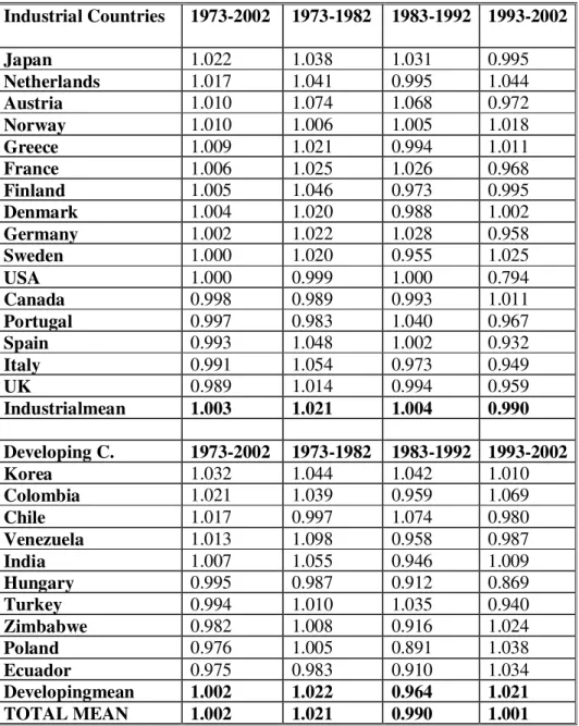
2.2. Contributions to Manufacturing Employment
It is important to examine the employment created in the automotive sector. The industry generates employment opportunities for the manufacturers, dealers, retailers, engineers, and electricians in the automotive sector. In addition, employment is created in related sectors, such as advertising, carpeting, textiles, computer chips, rubber, glass, lead, iron, steel, recycling, fuel, and others. Including related industries, it is estimated that each direct position in the automotive sector supports at least another five indirect jobs in related manufacturing and service industries.
The automotive sector is one of the major industries in most countries in terms of its share of employment. In the years included in the analysis, the sector accounted for approximately 10% of the total employment in all manufacturing. Table 3 shows employment shares of the sectors in total manufacturing employment.
Table 3: Sectoral Employment Shares in Total Manufacturing
Sector 1981(%) Rank 1990(%) Rank 2000(%) Rank
311 9.58 4 9.87 4 11.76 1 313 1.25 20 1.09 20 1.07 20 314 0.90 23 0.86 23 0.98 21 321 8.24 5 7.23 5 5.94 6 322 4.53 8 4.29 8 4.07 8 323 0.55 24 0.50 24 0.48 24 324 1.05 21 0.92 21 0.92 22 331 2.50 14 2.37 15 2.78 16 332 1.94 17 2.00 17 3.05 11 341 2.80 13 2.73 13 2.81 14 342 4.37 9 5.19 7 3.21 10 351 2.81 12 2.67 14 2.24 17 352 2.90 10 3.13 11 3.73 9 355 1.43 19 1.53 19 1.27 19 356 2.30 15 3.20 10 4.28 7 362 0.97 22 0.89 22 0.86 23 369 2.87 11 2.80 12 3.03 12 371 4.98 7 3.59 9 2.80 15 381 6.86 6 7.08 6 9.27 3 382 11.02 1 11.10 1 10.31 2 383 9.87 3 10.33 2 9.18 4 384 9.89 2 9.95 3 8.98 5 385 1.97 16 2.35 16 2.94 13 390 1.66 18 1.67 18 1.74 18 Others 2.62 2.54 2.18 Total 100 100 100
Source: UNIDO INDSTAT3 rev.2, 2006.
The table shows that approximately 9.9% of total manufacturing employment is situated in the automotive sector in 1981. With this share, the automotive sector is ranked second after “Machinery, Except Electrical.” In 1990, although its rank declined to third, the share of the automotive sector in total manufacturing employment increased slightly to 9.95%. In 2000, it is ranked fifth with a small decline both in share and in rank, and captured 8.98% of total manufacturing employment.
Country-by-country results reveal the contribution of the sector to the employment levels of the countries.6 Data show that, in 2000, for more than half of the countries, the automotive sector is among the top five sectors with the largest employment shares.
Since the automotive sector is an industry which is very open to technological changes, this decline in total employment share, which is accompanied by a small increase in production share, may be the result of labor-saving technological changes in automotive production. By comparing Tables 4, 5, and 6 in Appendix A, we can conclude that country-by-country results also support this idea; among the individual countries, the technologically-leading countries of the world, such as USA, the UK, France, Italy, and Spain, have also experienced declines in share of employment in the automotive sector. The emerging markets of the sector, such as Korea, Turkey, India, and some of the formerly communist countries, Hungary and Poland, also have experienced declines in the employment share of the automotive sector with an increase in production share.
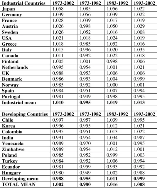
2.3. Contributions to Manufacturing Exports
International trade is another area where the importance of the automotive sector can be seen easily. Furthermore, recent changes in the world division of labor can be traced to changes in exports.
6
The detailed employment analyses for each country for the years 1981, 1990, and 2000 can be found in Tables 4, 5, and 6 of Appendix A, respectively.
Table 4 shows that, in 1981, the automotive industry captured a 20.37% share of world manufacturing exports. In 1990, it showed an increase and achieved a 21% share in total manufacturing exports. In 2000, although it showed a decrease and declined to 18.79%, for all three years, the sector is ranked first in total manufacturing exports in the world.
The contribution of the industry to the export levels of countries cannot be underestimated. For more than half of the countries in the sample, the automotive sector export share is in the top three of total manufacturing exports.7
For Turkey, in 1981, the sector is ranked fifth with a share of 5.6% of the country’s total manufacturing exports. In 1990, the share of the sector increased to 8.9% and it is ranked first. Table 9 in Appendix A shows that in 2000, with a share of 10.7%, it is ranked as the third sector in Turkish total manufacturing exports after the “Textiles” and “Wearing Apparel, Except Footwear” sectors. These increasing export shares show the growing impact of the sector on the Turkish economy. Founded as a montage industry in the beginning of the 1960s, according to Taskin (2004), the sector was able to export only 2% of its production by 1993. But today, the industry is one of the driving forces of the Turkish economy given its export levels.
7
Export shares and rankings of the sectors in total manufacturing of the countries for the years 1981, 1990, and 2000 are presented in tables 7, 8, and 9 of Appendix A, respectively. Since the export data are not available for Hungary and Poland in all three years, for Zimbabwe in 1981 and 2000, and for Germany in 2000, total export values are calculated using the data of remaining countries.
Table 4: Sectoral Export Shares in Total Manufacturing
Sector 1981(%) Rank 1990(%) Rank 2000(%) Rank
311 6.23 6 4.56 5 3.30 8 313 1.00 17 1.06 17 0.87 18 314 0.35 24 0.52 23 0.32 24 321 4.60 7 4.05 7 3.38 7 322 1.41 14 1.97 12 1.57 13 323 0.45 23 0.52 23 0.49 23 324 0.68 21 0.73 21 0.52 22 331 1.43 13 1.36 14 1.16 14 332 0.74 20 1.00 19 0.97 17 341 3.57 9 3.62 8 2.82 9 342 0.79 19 0.93 20 0.73 20 351 8.88 4 8.78 4 7.28 4 352 2.89 11 3.38 10 3.98 6 355 1.25 15 1.15 16 1.03 16 356 0.83 18 1.29 15 1.11 15 362 0.62 22 0.70 22 0.55 21 369 1.17 16 1.02 18 0.76 19 371 6.63 5 4.13 6 2.70 11 381 4.05 8 3.54 9 2.79 10 382 17.35 2 18.48 2 17.23 3 383 9.38 3 11.96 3 17.58 2 384 20.37 1 21.00 1 18.79 1 385 3.41 10 2.72 11 4.27 5 390 1.80 12 1.41 13 1.78 12 Others 5.22 2.66 3.90 Total 100 100 100
Source: UNIDO IDSB 2007.
Table 5, which presents the export shares of total automotive exports for the countries in our sample, shows that the largest share of automotive exports belongs to Japan, with 24%, and the second largest is USA with 21%. This is followed by West Germany, with 18% in 1981. Even though by the year 2000, USA and Japan changed rankings, the same three countries continued to be the three major exporters among automotive producers. The industrial countries in the sample account for 98.6 % of total exports in 1981 and 94.5% in 2000. In the
same period, the share of the developing countries in our sample increased from 1.4% to 5.5% showing a fourfold improvement.
Table 5: Country Shares in World Automotive Exports
COUNTRY 1981 (%) 1990 (%) 2000 (%) USA 20.91 19.20 23.55 JAPAN 24.29 19.37 20.78 CANADA 7.29 8.68 13.26 FRANCE 8.90 10.03 11.68 UK 6.89 5.32 6.71 SPAIN 1.50 3.36 5.70 ITALY 4.37 5.01 5.26 NETHERLANDS 1.57 0.24 2.23 AUSTRIA 0.46 0.79 1.67 SWEDEN 2.72 2.32 1.64 PORTUGAL 0.08 0.32 0.69 FINLAND 0.59 0.55 0.52 NORWAY 0.64 0.52 0.37 DENMARK 0.57 0.36 0.36 GREECE 0.03 0.02 0.05 GERMANY 17.74 22.02 Na Total Industrial 98.60 98.10 94.50 KOREA 1.07 1.65 4.67 TURKEY 0.07 0.064 0.48 INDIA 0.15 0.13 0.22 CHILE 0.04 0.009 0.05 COLOMBIA 0.01 0.003 0.05 VENEZUELA 0.03 0.01 0.04 ECUADOR 0.000 0.000 0.01 ZIMBABWE Na 0.000 Na POLAND Na Na Na HUNGARY Na Na Na Total Developing 1.40 1.90 5.50 Total 100 100 100
Source: UNIDO IDSB 2007.
Export share results parallel those of production results. Again, USA, Japan, and Germany are the leading countries in world automotive exports. The other big exporters are the UK, France, Italy, Canada and Spain. All developing
countries increased their export shares in 2000, as compared to 1990. Among developing countries, Turkey has the second largest share after Korea in total automotive exports, with an increasing trend through the years. In 2000, Turkey achieved a 0.48% share of total automotive exports and this was more than seven times the share in 1990. Additionally, Korea experienced a huge increase in export share, from 1.65% in 1990 to 4.67% in 2000. This shows that emerging countries have started to compete with the large producers in the industry.
Results of the analyses show the importance of the sector both for the global economy and for the individual countries. Sectoral comparisons indicate that the sector is one of the largest industries in the world in terms of its employment, production, and export levels.
Country-based results show the automotive industry to be dominated by a few countries. But the emerging countries have started to have a presence in the global automotive market in the last years with their production and export shares. If they continue to make technological and strategic connections with the leading countries in the sector, they can increase their importance and weight in the global market.
CHAPTER III
LITERATURE REVIEW
3.1. Productivity Literature
In this chapter, we give a literature review on the methodology we use to compute productivity changes, namely the Malmquist Productivity Change Index, based on Data Envelopment Analysis (DEA), and explain the reasons for choosing this approach.
Productivity is a very important indicator for the economic improvement of a country or a sector. Especially for a sector like automotive, whose contributions to the economy cannot be underestimated, productivity analysis is necessary. But surprisingly little research has been done on automotive sector productivity analysis.
Since there is no research investigating cross-country differences in the automotive sector on a global level, this paper intends to fill this void by using a productivity change method that we believe is the best.
In the productivity literature, there are two main approaches for measuring productivity growth: partial factor productivity measures, and total factor productivity measures. Partial factor productivity measures, such as labor
productivity (output per unit of labor input) and capital productivity (output per unit of capital input)are although commonly used in the productivity literature, they are, as the names suggest, only partial indices and thus can give misleading interpretations for overall productivity level. For example, labor productivity is affected by other inputs in production. Changes in capital input or intermediate inputs also affect the labor productivity. Hence, a productivity measure involving all factors of production, namelytotal factor productivity (TFP), is a more reliable measure of productivity.
The first approach to calculating TFP is the parametric method based on the estimation of some function, such as a production or cost function, and the second approach is based on the construction of an index number using non-parametric methods. Since the first approach requires imposition of a functional form for production technology, which is a strong assumption, we followed the nonparametric approach.
Among the productivity change indices, the Fisher (1922), Törnqvist (1936), and Malmquist (1953) indices are the most frequently used. Under certain conditions, the Malmquist index can be related to the Törnqvist and Fisher indices. Caves et al. (1982) showed that the Malmquist index is equivalent to the Törnqvist index if technology is translog, firms are cost minimizers, and profit maximizers, and second order terms are constant. Furthermore, Balk (1993) generalized the conditions explained by Färe and Grosskopf (1990) for calculating the Malmquist index as a quotient of the Fisher ideal index, and showed that if there is no allocative efficiency, these two indices are approximately equal.
We choose to use the Malmquist index for our productivity change analysis because it has a number of desirable properties, which makes it preferable over the Fisher and Törnqvist indices.
The Malmquist index was originally constructed by Sten Malmquist (1953) as a quantity index for consumption analysis. In their 1982 paper, Caves et al. adapted this consumption index to production analysis. In 1989, Färe et al. show the computation of this Malmquist productivity index using non-parametric linear programming methods.
The Malmquist index has many useful properties. As stated in Grifell-Tatjé and Lovell (1996), it does not require cost minimization or profit maximization and does not require any price information of inputs and outputs. At the same time, it can be used for multiple input and multiple output cases without aggregation problems.
Moreover, since the Malmquist index is constructed by means of a frontier model, it has the advantage of allowing for inefficient performance. The non-frontier productivity change measures, such as the index number approaches (like the Divisia and Törnqvist indices) or standard growth accounting approach (e.g. Solow (1957); Denison (1972)), assume that all individuals are efficient. So, in the existence of inefficiency, the estimation of technical progress would be biased. Furthermore, even in the absence of technical inefficiency, the TFP growth accounting estimation would be biased if the individuals are not cost minimizers; that is, if there is allocative inefficiency. As an example, Färe et al. (1994a) showed the relationship between the Malmquist index and traditional measures of productivity growth by a
Cobb-Douglas production function. They stated that in the presence of inefficiency the Cobb-Douglas approach gives a biased estimate of technical change.
Maybe the most desirable feature of the Malmquist index is its decomposability. The first study decomposing productivity change into technical change and efficiency change was by Nishimizu and Page (1982). In this first decomposition however, a functional form specification for technology was required. In their 1989 paper, Färe et al. showed the decomposition of the Malmquist index into efficiency change and technical change by using non-parametric methods. By means of this new decomposition method, it became possible to see, without a necessity to estimate the technology parameters, whether productivity has improved through technological improvements (technical change) or through a more efficient use of the current technology (efficiency change).
To compute the Malmquist index, we need to calculate distance functions, which are functional representations of multiple input/multiple output technology. To calculate distance functions, we use the same technique as Färe et al. (1994a), namely DEA methodology. DEA is a linear programming methodology to construct a nonlinear piece-wise frontier over the data. The method received attention after Charnes et al. (1978) employed it and in where the term DEA was first used.
As stated in Coelli et al. (2005), “An introduction to efficiency and productivity analysis,” one can also calculate distance functions using stochastic frontier approaches (SFA), which have the advantage of dealing with measurement error, but on the other hand, require imposing a particular
functional form for the production function and specifying distributional assumptions to separate the distance to the frontier function from measurement error.
3.2. TFP Literature
In the productivity literature there are many methods to measure TFP. For example, Mello (1999), “Foreign direct investment-led growth: evidence from time series and panel data” estimates the impact of foreign direct investment (FDI) on TFP growth for a sample of 32 OECD and non-OECD countries over the period 1970-90, where TFP growth is measured as the difference between per capita output growth and per capita capital accumulation. Results show a positive relationship between FDI and TFP for OECD countries, but a negative relationship for non-OECD countries.
“The creation and spread of technology and total factor productivity in China’s agriculture” by Jin et al.(2001), uses the Divisia index for TFP measurement for the period 1982-1995. The results indicate that China’s TFP for rice, wheat and maize grew rapidly and new technology accounts for most of the productivity growth. Moreover, in the paper “Subsidy and productivity in the privatised British passenger railway”, (Cowie, 2002) productivity is examined through the use of a Törnqvist productivity index.
Lederman et al. (1999), in their paper “Economic reforms and total factor productivity growth in Latin America and Caribbean, 1950-95: An empirical
note,” used the growth accounting approach based on the assumption that the production function follows a Cobb-Douglas form.
Using a stochastic frontier production function, Coelli et al. (2003) examined productivity growth in Bangladesh crop agriculture for the period 1961-1992, using data from 16 regions. Results show a productivity decline on the average during the period of study. Another paper using SFA, “A decomposition of TFP growth in Korean manufacturing industries: A stochastic frontier approach” by Kim and Han (2001), applied the stochastic frontier production model to Korean manufacturing industries. The paper decomposed total factor productivity into efficiency change, technical change, allocative efficiency change and scale efficiency change for the years 1980-1994, and showed that the main reason for productivity growth was technical progress.
3.3. Applications of the Malmquist Index
As we stated previously, the Malmquist index has very important advantages compared to other productivity measures. Thus, it has many applications to sectoral level productivity analyses.
Perhaps the most common use of the Malmquist index is in the banking sector. For example, “The sources of productivity change in Spanish banking”, (Grifell-Tatje, Lovell, 1997), “Efficiency and Productivity Growth in Turkish Commercial Banking Sector: A non-parametric approach”, (Fethi et al., 1998), “Measuring Productivity Changes in Australian Banking: An Application of Malmquist Indices” (Sathye, 2002), are some papers using the DEA-based Malmquist index in the banking sector.
Moreover, in their 1996 paper “Deregulation and productivity decline: The case of Spanish savings banks,” Grifell-Tatje and Lovell examined TFP change in Spanish savings banks for the period 1986-1991 using the Malmquist index and found that liberalization of Spanish savings banks led to productivity declines. They explained their reason for choosing the Malmquist index as the productivity measure instead of the Törnqvist index, by citing the three main advantages of the Malmquist index. Specifically, the Malmquist index does not require price information on resources used and services provided, it decomposes productivity change into technical change and efficiency change and it does not require the assumption of profit maximization. The latter is an especially important feature of the Malmquist index for the authors, because the savings banks are not profit maximizers; consequently, it would be inappropriate to use an intertemporal profit function or Törnqvist productivity index, which requires cost minimization and revenue maximization, as a productivity measure.
Agriculture is another sector using the Malmquist index for productivity analysis. Coelli and Rao (2003) investigate productivity growth in the agriculture sectors of 93 developed and developing countries for 1980-2000 using the DEA-based Malmquist index. Results show positive productivity growth on the average, mostly due to technical change. Moreover, Nkamleu (2003), “Productivity growth, technical progress and efficiency change in African Agriculture” and Fulginiti and Perrin (1997), “LDC agriculture: nonparametric Malmquist productivity indexes” are two other cross-country studies on productivity in the agriculture sector.
The 1992 paper of Färe et al., “Productivity changes in Swedish pharmacies, 1980-1989: A nonparametric Malmquist approach,” applied a DEA-based Malmquist index methodology to a panel data of Swedish pharmacies. By imposing a separability assumption on the distance functions, the authors decompose the Malmquist index into three components, namely, quality change, technical change and efficiency change. Results show that the data are not consistent with separability, since productivity growth changes according to the imposition of the separability assumption.
The Malmquist productivity index has a very wide range of sectoral applications for productivity analyses. We can name “Productivity development of Norwegian electricity distribution utilities” (Førsund and Kittelsen, 1997), “Productivity developments in Swedish hospitals: A Malmquist output index approach” (Färe et al., 1994b), “A comparative performance of the public enterprise sector in Turkey: A Malmquist productivity index approach” (Taskin, Zaim, 1997), “Productivity growth in health-care delivery” (Färe et al., 1997), “Productivity and quality changes in Swedish pharmacies” (Färe et al, 1994), “DEA-Malmquist productivity measure: New insights with an application to computer industry” (Chen and Ali, 2003), among others.
The Malmquist productivity index is used not only at the sectoral level, but also in aggregate level productivity analyses. For example, “The global trends of total factor productivity: Evidence from nonparametric Malmquist index approach” by Kruger (2003), investigated the productivity change in 87 countries for the period 1960-1990. The author states that the DEA-Malmquist approach has substantial advantages compared to traditional growth accounting,
since it does not rely on questionable equilibrium assumptions to merge multiple inputs into a single index and it can decompose the productivity change into technical change and efficiency change. Results show that technological progress occurs only in OECD countries and therefore in the range of relatively high capital intensity.
Moreover, “Total factor productivity measurement and human capital in OECD countries” Pastor et al. (1999), used the Malmquist index, including human capital, to calculate productivity in OECD countries for the period 1975-1990. Results indicated the existence of a significant effect on TFP associated with human capital.
3.4. Literature on Automotive Sector Productivity
Productivity analysis of the automotive sector usually uses labor productivity as a productivity measure. However, as we stated earlier, partial productivity measures may give misleading results, so TFP analyses are necessary. Moreover, perhaps due to the difficulty of finding cross-country comparable sectoral level data, analyses usually focus on specific regions and subsectors. Consequently, there is no research investigating global productivity trends of in the automotive industry.
The research on productivity in the automotive sector includes “Inventory Reduction and Productivity Growth; Linkages in the Japanese Automotive Industry”, a paper by Lieberman and Demeester (1999). The paper used data for fifty-two Japanese automotive companies for the period 1965-1991 to evaluate
the inventory reduction and productivity relationship. In that paper, productivity is measured by labor productivity, which is defined as real value added per employee. It is found that firms increased their productivity rank during periods of substantial inventory reduction.
“Inventory reduction and productivity growth: A comparison of Japanese and US automotive sectors” by Lieberman and Asaba (1996), examines the inventory and productivity performances of the Japanese and US automotive sectors for the period 1967-1993. As a productivity growth measure, the authors used labor productivity and find a strong relationship between inventory reduction and productivity growth for the automotive sectors of both countries.
The productivity analyses on the sector usually focus on specific subsectors of the automotive industry, such as automobiles. For example, the 1990 paper of Lieberman, Lau and Williams: “Firm level productivity and Management Influence: A comparison of US and Japanese Automobile Producers” compares six major US and Japanese motor vehicle manufacturers for the period 1950-1987. To calculate productivity, labor, capital, and total factor productivity are used, where TFP growth is a weighted average of the growth rates of labor and capital productivity. It is found that improvements in productivity were the result of more efficient use of labor and for most of the firms, long-run growth in capital productivity was negligible.
Another research effort on automobiles is “International Relations and Productivity in the US Automobile Industry” (Kochan et al.(1987). In this paper, the authors investigated labor productivity for one American automobile
manufacturer’s 53 plants for the period 1979-1986. Their results indicated negative effects of work teams on plant productivity.
Two 2002 papers by Ito “Are foreign multinationals more efficient? Plant productivity in the Thai automobile industry” and “Foreign ownership and productivity in the Indonesian automobile industry: Evidence from establishment data for 1990-1999” investigate the productivity differences between the foreign and local plants in the Thai and Indonesian automobile industries, respectively. For productivity calculations both labor productivity and total factor productivity, which is measured by the Törnqvist index, are used. In both papers, both labor productivity and TFP results reveal no evidence that foreign plants have relatively high productivity that can be related to their ownership-specific advantages.
Another paper by Ito (2004) “Foreign ownership and plant productivity in the Thai automobile industry in 1996 and 1998: A conditional quantile analysis” also investigates productivity differences between foreign and local plants in Thailand using labor productivity and a Törnqvist-Thail translog index of TFP; it confirmed the results of his 2002 paper.
Some research concentrates on automotive components industry. For example, “Foreign direct investment and host country productivity: the American automotive component industry in the 1980s” by Chung et al. (2003) examined the productivity of the US auto-component industry for the years 1979-1991 by estimating a log-linear Cobb Douglas production function to calculate productivity. The paper finds no evidence of direct technology transfer affecting the productivity of US suppliers.
“Product variety and manufacturing performance: Evidence from the international automotive assembly plant study” by MacDuffie et al. (1996), presents the cross-sectional examination of assembly plant productivity for the period 1985-1990, which is measured by labor productivity. Results indicated that an intermediate type of product variety negatively affects productivity.
CHAPTER IV
METHODOLOGY
To investigate productivity differences across countries, we use a non-parametric Malmquist productivity change index. In Chapter 3, by means of the productivity literature, we explained several advantages of this approach over other productivity change measures. In this chapter, we show the composition of this index and computation of it using linear programming techniques.
Formally, in order to define the output-oriented Malmquist index, we must first define the concept of output distance functions. An output distance function is the reciprocal of the maximal proportional expansion of the output vector, given input vector.8 Hence, it is formulated as,
(
)
{
}
(
sup : ,)
inf{ :( , / ) } ) , ( t t t t t 1 t t t t o x y x y S x y S D = θ θ ∈ − = θ θ ∈where St is the production technology at time t, defined as
8
An input distance function, on the other hand, describes the production technology by looking at the minimally possible proportional contraction of the input vector, given the output vector. The two measures provide the same technical efficiency scores when a constant returns to scale (CRS) technology applies, which is the case in this paper. For a further discussion of the input-oriented distance function, see Deaton (1979).
St = {(xt,yt) : xt can produce yt }, t=1,2,…,T,
and xt and yt are the input and output vectors at time t, respectively. Following Färe et al. (1994) we can write the Malmquist index as,
2 / 1 1 1 1 1 1 1 1 1 ) , ( ) , ( ) , ( ) , ( ) , , , ( = + + + + + + + + t t t o t t t o t t t o t t t o t t t t o y x D y x D y x D y x D y x y x M where t( t 1, t1) inf{ :( t 1, t 1/ ) t} o x y x y S D + + = + + ∈ θ θ and +1( , ) inf{ :( , / ) +1} ∈ = t t t t t t o x y x y S D θ θ .
Note that, the distance function t( t+1, t+1)
o x y
D describes the maximal
proportional change in output, required to make( t+1, t+1
y
x ) feasible in relation to
the technology at t.
The Malmquist index methodology allows us to decompose productivity change into its efficiency change and technical change components. So, after some basic manipulations we get,
2 / 1 1 1 1 1 1 1 1 1 1 1 1 ) , ( ) , ( ) , ( ) , ( ) , ( ) , ( ) , , , ( = + + + + + + + + + + + t t t o t t t o t t t o t t t o t t t o t t t o t t t t o y x D y x D y x D y x D y x D y x D y x y x M
Efficiency Change Technical Change
In the present methodology, a world frontier is constructed using the data of the countries in the sample, and then each country is compared to that world frontier. In the formulation of the Malmquist index above, the first term measures whether the observed production of a country is getting closer to the world frontier between periods t and t+1, i.e., efficiency change. The second
term captures the technical change, i.e. shifts in the world frontier, so an improvement in this index is evidence of “innovation”.
To be more informative, we can explain the framework for constant
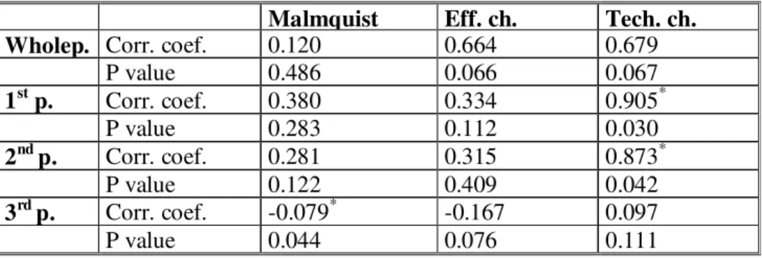
returns to scale technology with Figure 1 below.9
Figure 1: The Malmquist Productivity Change Index
In the figure, Ft and Ft+1 are world frontiers for the periods t and t+1, respectively. Now, for any given country represented by (xt,yt) in period t, the
output bundle yt is inefficient because the country can produce b instead of yt,
without changing input bundle xt and the technology level. The distance
9
Source of the figure and the concept explained in this chapter is Färe et al., (1994). F t f X xt+1 xt 0 St+1 St yt+1=e d c b yt=a Ft+1 (xt+1,yt+1) (xt t y , ) Y
function Dt( t, t)
o x y is the reciprocal of the maximal ray expansion (or
contraction) of yt given xt , so the value of this function is ob oa
, which is less
than 1. Note that t( t, t)≤1
o x y
D if and only if, (xt,yt) ∈ St, and t( t, t)=1
o x y
D if
and only if (xt, yt) is on the frontier, that is, if technical efficiency exists.
Furthermore, in the figure (xt t
y , ) t S ∈ and (x +1, t+1 y t ) +1 ∈ t S , but (xt+1, t+1
y )∉St, so we conclude that technical progress has occurred. Moreover,
Dt( t+1, t+1)
o x y , the distance function evaluating (x
1 1
, + + t
t y ) relative to the period t
technology level, is oc oe
, which is greater than 1.
Therefore, if we write the Malmquist index in terms of distances in the figure, it becomes, M = ob oa of oe 2 / 1 od oa ob oa of oe oc oe .
Malmquist index values greater than unity indicate positive productivity growth between the two periods, t and t+1, and values less than unity suggest the converse. Similarly, improvements in the components of the Malmquist index yield values greater 1 of those components, and deteriorations yield values less than 1.
By comparing the values of technical efficiency change and technological change, we can understand the sources of productivity gains or losses. For instance, if the technical efficiency component is greater than the technological change component, then we can conclude that productivity gains are the result of efficiency improvements.
The calculation of the Malmquist index requires the solution of a sequence of linear programming problems. Assuming there are k=1,2,…,K observations (in our case, countries), N inputs and M outputs, and imposing constant returns to scale and strong disposability of technology, the following
linear programs are computed to calculate the productivity of observation ko
:
[
( , , , )]
1 maxθ
= − t k t k t o O O y x D subject to 0 , 1 , −∑
= ≤ t m k K k k t m k y y Oλ
θ
, m = 1,2,…,M 0 , , 1 − ≤∑
= t n k t n k K kλ
kx x O , n = 1,2,…,N (1) 0 ≥ k λ , k = 1,2,…,K[
1( , 1, , 1)]
1 maxθ
= − + + + k t k t t o O O y x D subject to 0 1 , 1 1 , − ≤ + = +∑
t m k K k k t m k y y Oλ
θ
, m = 1,2,…,M 0 1 , 1 , 1 − ≤ + + =∑
t n k t n k K kλ
kx x O , n = 1,2,…,N (2) 0 ≥ kλ
, k = 1,2,…,K[
( , 1, , 1)]
1 maxθ
= − + + k t t k t o O O y x D subject to 0 , 1 1 , −∑
= ≤ + t m k K k k t m k y y Oλ
θ
, m = 1,2,…,M 0 1 , , 1 − ≤ + =∑
t n k t n k K kλ
kx x O , n = 1,2,…,N (3) 0 ≥ k λ , k = 1,2,…,K[
1( , , , )]
1 maxθ
= − + k t k t t o O O y x D subject to 0 1 , 1 , − ≤ + =∑
t m k K k k t m k y y Oλ
θ
, m = 1,2,…,M 0 , 1 , 1 − ≤ + =∑
t n k t n k K kλ
kx x O , n = 1,2,…,N (4) 0 ≥ kλ
, k = 1,2,…,Kwhere t = 1,2,…,T, and
λ
k indicates at what intensity a country may beemployed in production. In programs (1) and (2) the observation and the technology are from the same period, so the value of the Malmquist index is less than or equal to unity. Where linear programs (3) and (4) occur, the observation is from one period, but the reference technology is from another period.
Note that, to this point, we have assumed a constant returns to scale
technology. By adding the convexity constraint
∑
1 =1=
K
k
λ
k in all of the linearprogramming programs above, we can obtain efficiency scores relative to a variable returns to scale technology, and thus can decompose the overall efficiency change (the change in efficiency calculated relative to the constant
returns to scale technology) into scale efficiency change and pure efficiency change components.
The pure efficiency component is the technical efficiency calculated under VRS technology, and scale efficiency is the component that captures the deviation between VRS technology and CRS technology at the observed inputs. An increase in scale efficiency means that the country has moved to a position with a better input/output quantity ratio at the frontier, conditioned on its input/output mix.
By running programs (1) and (2) with and without convexity constraints, we can measure pure technical efficiency change (PEFFCH) and overall techni- cal efficiency change (EFFCH), respectively. Scale efficiency change (SEFFCH) can be obtained by dividing overall technical efficiency change by pure technical efficiency change. Therefore, we can write that;
EFFCH = PEFFCH * SEFFCH.
Then, using the same logic as above, if the pure technical efficiency index is greater than the scale efficiency index, we can say that the source of the efficiency change is an improvement in pure technical efficiency.
Now we apply this procedure to the data of 26 selected countries. But first let us mention the data.
CHAPTER V
DATA
To compute the Malmquist productivity change index, we need output, labor and capital stock data at the sectoral level, comparable across countries and over time. Our data source is United Nation’s Industrial Statistics database (INDSTAT3 2006 ISIC rev.2), and data are defined at the three-digit level of the International Standard Industrial Classification (ISIC) code. Although this data source covers the period 1963-2004 for a set of 181 countries, for the majority of the countries, data are not available for a large proportion of this time span. Hence, we choose countries in our sample according to availability of sector level data in the data set. To get the most reliable results, we restricted our data
set to 26 countries over the time period from 1964 to 2002.10
The set of countries is reported in Table 6 with their value added/labor indices in the automotive sector for years 1981, 1990, and 2000. This index is calculated using the formula:
10
Moreover, for the data of 10 countries we made estimations to complete the missing data for labor, output, and invesment. To complete output and labor data, we fitted the linear functions Y=a+bT and L=c+dT, respectively, where T is the time trend. To complete investment data, first we found the average of available i ratios for each country, where i=I/Y, and then we used this ratio to calculate unavailable I levels using I=i*Y.
Ii = (Value Addedi/Labori)/ (Value AddedTurkey/LaborTurkey)*100, where i represents the country and for Turkey it takes the value 100. So the index indicates the performance of the automotive sectors of countries relative to that of Turkey.
Table 6: Relative Value Added/Labor Indices in Automotive Sectors
COUNTRY VA/L Index
1981 VA/L index 1990 VA/L index 2000 AUSTRIA 627.218 703.489 625.249 CANADA 2033.609 1678.374 2332.769 DENMARK 883.834 722.284 556.780 FINLAND 1261.429 927.880 311.905 FRANCE 2134.887 1660.237 948.549 GERMANY 2791.053 2794.371 2224.600 GREECE 365.112 158.183 123.485 ITALY 1217.444 844.371 451.543 JAPAN 2395.414 2547.038 1952.448 NETHERLANDS 712.932 542.462 397.841 NORWAY 1689.549 797.597 1021.281 PORTUGAL 239.022 192.165 262.473 SPAIN 727.819 874.292 539.939 SWEDEN 3001.955 2484.036 1508.540 UK 2108.797 1655.267 910.628 USA 2861.353 1979.724 1779.206 Industrial mean 1565.714 744.809 996.702 CHILE 130.075 38.117 52.517 COLOMBIA 74.360 31.369 14.365 ECUADOR 26.616 6.978 4.084 HUNGARY 361.954 125.773 258.110 INDIA 13.909 9.084 5.778 KOREA 690.300 1673.700 2562.451 POLAND 416.466 160.204 119.586 TURKEY 100 100 100 VENEZUELA 370 33.015 83.870 ZIMBABWE 52.180 25.246 18.867 Developing mean 223.586 204.278 321.962
According to the table,11 Turkey is one of the worst performing countries in terms of value added per labor in the automotive sector. In 1981, out of 26 countries in the data set, only four countries had smaller index values than Turkey, which are Colombia, Ecuador, India, and Zimbabwe, all of which are developing countries. Value added per labor values for Japan, USA, Canada, the UK, Germany, France, and Sweden are more than 20 times that of Turkey’s value. This means that value added gains from automotive sector labor in these countries are 20 times more than gains from automotive labor in Turkey. On the average, the labor efficiency of industrial countries is sevenfold of that of developing countries. Countries like Korea, Hungary, Poland, and Venezuela, with which Turkey is expected to compete, also had greater values than Turkey’s. In 1990 and 2000, Turkey showed a better performance and lessened its differential versus other countries: in addition to the formerly mentioned four countries, Turkey’s labor efficiency performance exceeded those of Chile and Venezuela. Korea showed a great improvement and achieved the top rank in value added per labor value in the automotive sector in 2000.
For the automotive sector, we would like to have data on motor vehicles, parts, and accessories production. At a three-digit industry classification, this sector is grouped under code 384, which is the “Transport Equipment” sector. The definition of transport equipment covers shipbuilding and repairing, manufacture of railroad equipment, motor vehicles, motorcycles and bicycles,
11
Source of labor and value added data is INDSTAT3 2006, ISIC rev.2. Definitions of data are given in the Appendix B.