Solution methodologies for debris : removal during disaster response phase

SOLUTION METHODOLOGIES FOR DEBRIS

REMOVAL DURING DISASTER RESPONSE

PHASE

a thesis

submitted to the department of industrial engineering

and the graduate school of engineering and science

of bilkent university

in partial fulfillment of the requirements

for the degree of

master of science

By

Nihal Berkta¸s

July, 2014

I certify that I have read this thesis and that in my opinion it is fully adequate, in scope and in quality, as a thesis for the degree of Master of Science.

Assoc. Prof. Bahar Yeti¸s Kara(Advisor)

I certify that I have read this thesis and that in my opinion it is fully adequate, in scope and in quality, as a dissertation for the degree of Doctor of Philosophy.

Assoc. Prof. Oya Kara¸san(Co-Advisor)

I certify that I have read this thesis and that in my opinion it is fully adequate, in scope and in quality, as a thesis for the degree of Master of Science.

Assoc. Prof. Osman O˘guz

I certify that I have read this thesis and that in my opinion it is fully adequate, in scope and in quality, as a thesis for the degree of Master of Science.

Asst. Prof. M. Alp Ertem

Approved for the Graduate School of Engineering and Science:

Prof. Dr. Levent Onural Director of the Graduate School

ABSTRACT

SOLUTION METHODOLOGIES FOR DEBRIS

REMOVAL DURING DISASTER RESPONSE PHASE

Nihal Berkta¸s

M.S. in Industrial Engineering Supervisor: Assoc. Prof. Bahar Yeti¸s Kara

Co-Supervisor: Assoc. Prof. Oya Kara¸san July, 2014

During the disaster response phase of the emergency relief, the aim is to reduce loss of human life by reaching disaster affected areas with relief items as soon as possible. Debris caused by the disaster blocks the roads and prevents emergency aid teams to access the disaster affected regions. Deciding which roads to clean in order to transport relief items is crucial to diminish the negative impact of a dis-aster on human health. Despite the significance of the problem during response, in the literature debris removal is mostly studied in recovery or reconstruction phases of a disaster. The aim of this study is providing solution methodologies for debris removal problem in response phase. In particular, debris removal activities on certain blocked arcs have to be scheduled in order to reach a set of critical nodes such as schools and hospitals. Two mathematical models are developed with different objectives. The first model aims to minimize the total time spent to reach all critical nodes whereas the second minimizes weighted sum of visiting times where weights indicate the priorities of critical nodes. Since obtaining solu-tions quickly is important in the early post-disaster, heuristic algorithms are also proposed. Two data sets belonging to Kartal and Bakırk¨oy districts of ˙Istanbul are used to test the mathematical models and heuristics.

Keywords: Debris management, debris removal, relief transportation, node rout-ing.

¨

OZET

AFET M ¨

UDAHALE SAFHASINDA ENKAZ Y ¨

ONET˙IM˙I

˙IC¸˙IN C¸ ¨

OZ ¨

UM Y ¨

ONTEMLER˙I

End¨ustri M¨uhendisli˘gi, Y¨uksek Lisans Tez Y¨oneticisi: Do¸c. Dr. Bahar Yeti¸s Kara

E¸s-Tez Y¨oneticisi: Do¸c. Dr. Oya Kara¸san Temmuz, 2014

Afetten etkilenen b¨olgelere yardım ekibinin ve acil yardım malzemelerinin ula¸stırılması afet lojisti˘ginin en ¨onemli safhalarından birini olu¸sturmaktadır. Afetin sebep oldu˘gu enkaz, afetzedelere ula¸sımı zorla¸stırarak barınma, beslenme ve sa˘glık hizmetlerini geciktirmekte, can kayıplarını artırmaktadır. Literat¨urde ¸co˘gunlukla afet y¨onetiminin iyile¸stirme ve yeniden in¸sa safhasında ¸calı¸sılmı¸s enkaz kaldırma problemi, bu ¸calı¸smada m¨udahale safhasında incelenmi¸stir. Afet son-rasında pop¨ulˆasyonu ve ¨onemi y¨uksek olan hastane, okul gibi kritik noktalara en kısa s¨urede ula¸sılmasını ama¸clayan ve temizlenecek ayrıtlara karar vererek kritik noktalar arasında rota olu¸sturan matematiksel modeller geli¸stirilmi¸stir. Geli¸stirilen ilk modelde ama¸c fonksiyonu en son ula¸sılan kritik noktanın varı¸s za-manını enazlamaktır. Kritik noktalara a˘gırlıklar atanarak, a˘gırlıklı toplam varı¸s zamanını enazlamayı ama¸clayan ikinci bir model geli¸stirilmi¸stir. Bu modellerin testinde Kartal ve Bakırk¨oy il¸celerinin verileri kullanılmı¸stır. Afet ortamında hızlı karar almak b¨uy¨uk ¨onem arz etti˘ginden, kısa s¨urede iyi ¸c¨oz¨umler ¨uretebilecek sezgisel y¨ontemler geli¸stirilmi¸s, veri setleri ¨uzerinde test edilmi¸stir.

Anahtar s¨ozc¨ukler : Afet y¨onetimi, enkaz kaldırma, acil yardım ula¸stırma, d¨u˘g¨um rotalama.

Acknowledgement

I would like to express my gratitude to my advisor Assoc. Prof. Bahar Yeti¸s Kara for her guidance, patience and being there whenever I needed her. I would like to thank my co-advisor Assoc. Prof. Oya Kara¸san for her valuable ideas and support. It has been a grate experience to work with them.

I am grateful to Assoc. Prof. Osman O˘guz and Asst. Prof. M. Alp Ertem for accepting to read this thesis and for their valuable comments. I would like to thank Halenur S¸ahin and Fırat Kılcı for their support in this research.

I would like to acknowledge the financial support of The Scientific and Tech-nological Research Council of Turkey (TUBITAK).

I would like to thank ¨Oz¨um Korkmaz for her invaluable friendship and support on every subject during these last two years. I will never forget the sleepless nights we spent with her and Nil Karacao˘glu who made the hard times bearable with her laughter. I would like to thank my dearest friend Merve Meraklı for her love and support. I am grateful to my friends H¨useyin G¨urkan and O˘guz C¸ etin for the patience they have shown to all of my questions for the last five years. I am grateful to Burcu Tekin for the joy she brought during our study. I would like to thank Ramez Kian, Gizem ¨Ozbaygın, Esra Koca, Ece Demirci, ˙Irfan Mahmuto˘gulları, Meltem Peker, Sinan Bayraktar for their friendship and support during our graduate studies. I am also thankful to my homemate Bihter Da˘glar for her moral support.

I am most grateful to my family; my mother and my role model Hatice Berkta¸s for her eternal love and support, my father ˙Izzet Berkta¸s who motivates me with his spirit, my sister Seda Sezgin Berkta¸s for her helpful advice and encouragement, and my brother ˙Ihsan Berkta¸s although he will be judgmental about the language of this thesis.

Last but not least, I am deeply grateful to Mesut Kaya for his love, patience and understanding.

Contents

1 Introduction and Problem Definition 1

2 Literature Review 8

2.1 General Routing Problems . . . 8

2.1.1 Arc Routing Problems . . . 9

2.1.2 Node Routing Problems . . . 11

2.2 Relief Transportation/Distribution . . . 12

2.3 Debris Removal . . . 14

3 Model Development 17 3.1 First Model: Minimize Total Time . . . 23

3.2 Second Model: Minimize Weighted Sum of Visiting Times . . . . 27

4 Heuristic Algorithms 31 4.1 Constructive Heuristics . . . 32

CONTENTS vii

4.1.2 Weighted Shortest Distance Heuristic . . . 37

4.2 Improvement Heuristics . . . 39

5 Data and Computational Analysis 42 5.1 Data . . . 42

5.2 Computational Analysis . . . 46

5.2.1 Analyses on the First Model . . . 46

5.2.2 Analyses on the Second Model . . . 57

5.2.3 Performance of Minratio Heuristic . . . 68

5.2.4 Performance of Weighted Shortest Distance Heuristic . . . 73

List of Figures

1.1 Disaster Management Cycle . . . 2

1.2 Debris Related Operations in Disaster Timeline . . . 4

1.3 Seismic zone map of Turkey [1] . . . 5

2.1 Framework for disaster operations and associated facilities and flow [2] . . . 12

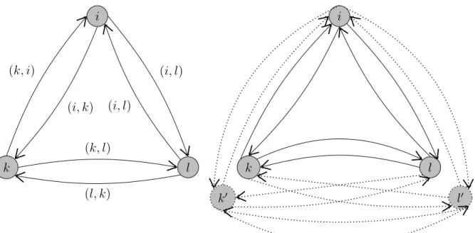
3.1 Original network G = (N, A) (left), new network (right) G0 = (N0, A0) where dotted nodes and arcs are artificial. . . 19

3.2 An example of revisiting a critical node where k, l, m ∈ C, i, j ∈ N C 26 4.1 A simple network where dashed edges show the shortest path be-tween each node . . . 33

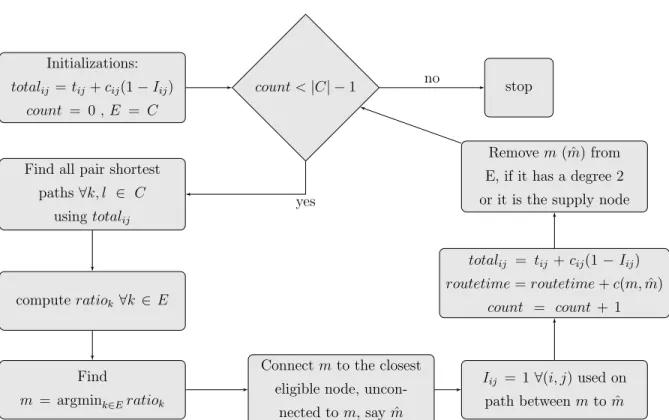
4.2 Flowchart of Algorithm Minratio . . . 35

4.3 Flowchart of Algorithm Weighted Shortest Distance . . . 38

4.4 An example of 2-opt applied on a feasible route . . . 39

LIST OF FIGURES ix

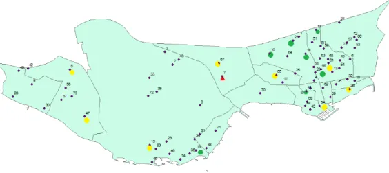
5.1 The location of supply node and critical nodes in Kartal . . . 44

5.2 The location of supply node and critical nodes in Bakırk¨oy . . . . 44

5.3 Optimal routes of instances K1,K2,K3,K4,K5 for MTT . . . 48

5.4 Example of constructing transportation network and T matrix . . 56

5.5 Optimal route of instance K7 for both of the mathematical models 62

5.6 Optimal route of B20 (schools) by MTT . . . 66

List of Tables

1.1 Debris Amount of Recent Disasters . . . 4

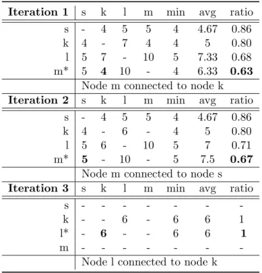
4.1 An example of Minratio Algorithm . . . 34

5.1 Features of the data set . . . 43

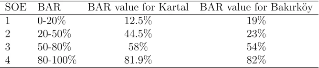
5.2 Severity of earthquake, corresponding BAR values and BAR values used in Kartal and Bakırk¨oy instances. . . 45

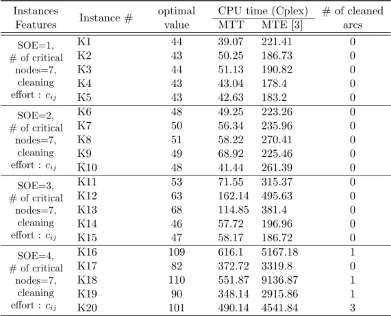
5.3 Performance of the first model on Kartal instances with higher cleaning times . . . 47

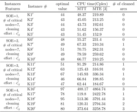
5.4 Performance of the first model on Kartal instances with lower cleaning times . . . 49

5.5 CPU times of models Minimize Total Effort [3] and Minimize Total Time (in seconds) . . . 49

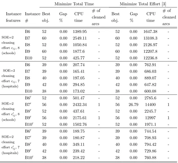
5.6 Performance of the first model on Bakırk¨oy instances with higher and lower cleaning times with SOE=1 . . . 51

5.7 Performance of the first model on Bakırk¨oy instances with higher and lower cleaning times with SOE=2 . . . 52

5.8 Performance of the first model on Bakırk¨oy instances with higher and lower cleaning times with SOE=3 . . . 53

LIST OF TABLES xi

5.9 Performance of the first model on Bakırk¨oy instances with higher and lower cleaning times with SOE=4 . . . 54

5.10 Performance of the first model on Bakırk¨oy instances with lower cleaning times and 15 critical nodes . . . 55

5.11 Performances of Cplex 12.6 and Gurobi 5 in terms of CPU times on Kartal instances with higher cleaning times with complete and transportation networks . . . 57

5.12 Performances of Cplex 12.6 and Gurobi 5 on Kartal instances with higher cleaning times for the second model . . . 58

5.13 Performance of the second model on Kartal instances with higher cleaning times . . . 59

5.14 Performance of the second model on Kartal instances with lower cleaning times . . . 60

5.15 Weights of the critical nodes in Kartal data set . . . 60

5.16 Total route times of optimal solutions obtained from the mathe-matical models using Kartal instances with higher cleaning times 61

5.17 Weights of the critical nodes in Bakırk¨oy (hospitals on the left, schools on the right) . . . 62

5.18 Performance of the second model on Bakırk¨oy instances (hospitals) with higher cleaning times . . . 63

5.19 Performance of the second model on Bakırk¨oy instances (hospitals) with lower cleaning times . . . 64

5.20 Performance of the second model on Bakırk¨oy instances (schools) with higher cleaning times . . . 65

LIST OF TABLES xii

5.21 Performance of the second model on Bakırk¨oy instances (schools) with lower cleaning times . . . 67

5.22 Comparison of Minratio, Maxratio and Avgratio on Kartal in-stances with higher cleaning times . . . 69

5.23 Performance of Minratio heuristic on Kartal instances with higher and lower cleaning times . . . 70

5.24 Performance summary and comparison of Minratio heuristics with the heuristic by S¸ahin [3] on Kartal instances . . . 70

5.25 Performance of Minratio heuristic on Bakırk¨oy instances with higher and lower cleaning times, critical nodes are schools . . . 71

5.26 Performance summary and comparison of Minratio heuristics with the heuristic by S¸ahin [3] on Bakırk¨oy instances (schools) . . . 71

5.27 Performance of Minratio heuristic on Bakırk¨oy instances with higher and lower cleaning times, critical nodes are hospitals . . . . 72

5.28 Performance summary and comparison of Minratio heuristics with the heuristic by S¸ahin [3] on Bakırk¨oy instances (hospitals) . . . . 72

5.29 Performance of Weighted Shortest Distance(WSD) heuristic on Kartal instances with higher and lower cleaning times . . . 73

5.30 Performance of Weighted Shortest Distance(WSD) heuristic on Bakırk¨oy instances (hospitals) with higher and lower cleaning times 74

5.31 Performance of Weighted Shortest Distance(WSD) heuristic on Bakırk¨oy instances (schools) with higher and lower cleaning times 75

Chapter 1

Introduction and Problem

Definition

Disaster operations include activities that are carried out before, during and after a disaster in order to reduce loss of human life, minimize the economical damage and restore the normal state or well-being of the community. Disasters could be natural and man-made; their timing and/or place might be known before-hand. While accidents and terrorist attacks fall into the man-made category, earthquakes and hurricanes are natural disasters for which the locations are pre-dictable. Regardless of the type of the disaster, the operations can be classified as pre-disaster and post-disaster operations. Disaster management cycle which includes these operations is mostly analyzed in four stages: mitigation, prepared-ness, response and recovery as in Figure 1.1. Mitigation consists of precautionary measures to avoid disaster or reduce its impact so mitigation activities take place both before and after a disaster. The purpose of preparedness activities is gaining the ability to respond and rescue when disaster strikes so it includes the activ-ities prior to a disaster. Response is the stage where resources are utilized to reach disaster area, save lives and prevent further economical and environmental damage. This stage is more complex since it takes place just after the disaster where resources should be activated immediately to reach affected people, re-alize the severity of the situation and plan accordingly. Recovery involves the

post-disaster activities to return to a normal state and provide stable life to the disaster victims [4]. Mitigation Preparedness Recovery Response Disaster

Figure 1.1: Disaster Management Cycle

Despite all kinds of precautions, disasters, especially natural ones are inevitable. Therefore planning disaster relief operations before it happens, and implementing them in early post-disaster phases are significant to diminish its impact. As stated by Wassenhove [5], huge part of disaster relief operations is about logistics. Hence to re-establish normal living conditions with the minimum loss of life and property we need to lead and carry out logistics operations effectively.

Sheu [6] defines emergency logistics as a process of planning, managing and con-trolling the flow of resources in order to provide relief and urgent services to affected people. Emergency logistics differs from the commercial supply chain due to the unique and extraordinary circumstances caused by disaster [7]. One of the challenges in emergency logistics is lacking capable resources to handle the situation or not being able to reach and activate them on time. During Haiti earthquake in 2010 the limited ramp space of the airport and lack of fuel prevented humanitarian flights from entering the country [8]. Furthermore the uncertain-ties about demand may result in wrong or excessive donations which complicate

handling and storage operations. For example, in Japan Earthquake in 2011 it is reported that too much blankets and clothing are donated. After the Joplin tornado happened in the same year, huge number of donations overwhelmed the storage and became an obstacle for distribution of actual needs [9].

Damage in communication systems and other infrastructure such as roads in-creases the complexity and difficulty in logistics. Again in Haiti earthquake the port was damaged and could not handle large ships so delivery of the emergency aids transported via ships were planned accordingly. Involvement of many parties to control these resources creates another challenge since they have to commu-nicate and coordinate efficiently. This challenge was sadly proved by Hurricane Mitch in 1998 when it took weeks for The International Federation of Red Cross and Red Crescent Societies (IFRC) to coordinate and distribute the donated reliefs [10].

When governments and institutions are not able to overcome these challenges, the effects of the disaster last for a long period of time, like in example of Haiti earthquake; 98% of the debris remained after six months from the earthquake and made the transportation impossible for the most part of the capital city [11]. Debris are caused by destruction of structures and vegetation and they block the roads and prevent accessibility to disaster affected areas. There are different type of debris; construction, vegetative, hazardous waste, properties such as white goods, vehicles etc. [12]. Hence debris differs from the normal waste in terms of content and amount as Hurricane Katrina proved it by producing more than fifty times the annual amount of daily solid waste in the U.S. in few hours [13].

The magnitude, type and place of a disaster change the characteristics of debris. For instance debris caused by an earthquake on an urban area mostly consists of ruins of buildings where hurricane debris contains trees, part of structures such as fences and rooftops, and other properties. Some of the recent worldwide disasters which caused high volume of debris can be seen in Table 1.1.

Table 1.1: Debris Amount of Recent Disasters

Year Event Debris Amount

2011 Japan Earthquake and Tsunami 250 million ton [14] 2008 Wenchuan Earthquake, China 380 million ton [15] 2005 Hurricane Katrina, USA 76 million m3 _[16]

2004 Indian Ocean Tsunami 10 million m3 _{(Only Indonesia) [17]}

2004 Hurricane Charley, USA 14 million m3 [18] 1999 Marmara Earthquake, Turkey 13 million ton [19] 1999 Chi-Chi Earthquake, Taiwan 20 million m3 _[20]

1995 Kobe Eartquake,Japan 15 million m3 [21] 1995 Hyogoken-Nambu Eartquake, Japan 2 billion ton [22]

There are different operations related to debris through the disaster timeline. In the pre-disaster phase considering possible disaster scenarios volume and char-acteristics of debris are estimated. Based on these estimations debris collection strategy is established. Recycling and collection sites are determined in this phase and necessary equipment is obtained. Just after the disaster, debris clearance starts in order to access affected areas and transport relief. Complete collec-tion and recycling of debris are the post-disaster operacollec-tions which usually take months. C¸ elik et al. [23] summarize these operations in Figure 1.2.

Clearance of debris after a disaster is a must to normalize the life of the victims. Debris have significant impact on people’s health both physically and mentally. While hazardous wastes threaten victims’ lives directly, living near the wreckages affects people’s psychology. These issues are the concerns of complete removal and recycle of debris in the post-disaster phase. Due to the nature of the response phase, the aim and characteristics of debris related activities are different. In this phase, the main purpose is to reach disaster affected areas in order to deliver relief. By relief we mean all kind of emergency aid items such as food and medicine. Hence the debris removal operations during this phase are only performed if it is necessary to reach an area and deliver relief as soon as possible.

In this study we focus on the debris removal or clearance operations in the re-sponse phase of a disaster, more precisely an earthquake. Earthquakes are not rare events; average annual number of earthquakes occurred worldwide in the last decade is 28 [24]. As it can be seen from the seismic zone map, Turkey is an earthquake prone country. Statistics show that in every 8 months a serious earthquake occurs in Turkey [25].

Coordination and execution of operations related to debris removal fall under responsibility of Republic of Turkey Prime Ministry Disaster and Emergency Management Presidency (T.C Afet ve Acil Durum Y¨onetim Ba¸skanlı˘gı)(AFAD). According to Turkey Disaster Intervention Plan published on May 2013 by AFAD, there are two main solution partners concerning these operations. Ministry of Transport, Maritime Affairs and Communication is responsible for providing fast and safe transportation to disaster areas by clearing debris, especially on the main roads. The duties of Ministry of Environment and Urban Planning are mostly related to the recovery phase such as debris removal after search and rescue operations, determining debris collection areas and destroying damaged buildings. There are other supportive ministries and sectors which coordinate with and provide equipments and personnel to AFAD.

Since the aim in disaster response phase is distributing relief to the people as soon as possible, the debris removal operations in this phase do not intend to clean all the blocked roads. Especially after a severe earthquake in a vulnerable area, unblocking all the road may take months. However people affected by the disaster need food, medicine, treatment, shelter etc. within minutes to fulfill basic needs. We call all of these needs as emergency aid or relief and in order to minimize the devastating effects of the disaster, these relief items must be delivered to the disaster affected people as soon as possible. For that purpose, complete clearance of the debris should be postponed to the post-disaster phase and roads should be cleaned only when it is necessary to use that road to enable accessibility a disaster affected region.

Reaching all the settlement areas of the disaster affected region in a short amount of time is not possible after a serious earthquake. Therefore we focus on a subset of them. This subset is called critical and it includes areas which are densely populated and consequently having an urgent need of relief items such as schools. Moreover, some areas are accepted as critical, such as hospitals and shelter areas, not only because they need urgent relief distribution but also they should stay open to public access. To enable transportation to these critical districts we have to decide which blocked roads to clean. Based on these concerns, Debris Removal Problem in Response Phase is defined as reaching a set of predetermined

critical disaster affected nodes as soon as possible by traversing arcs which may be blocked due to debris [3]. Hence to visit a critical node, we may chose to use a blocked arc but to be able to use a blocked arc we need to remove the debris on it in expense of some effort.

We assume that there is depot or supplier from which a vehicle departs and visits each critical node to deliver relief items. Once debris on a blocked arc are removed the arc remains clean. Thus, when a blocked arc is traversed for the first time, debris are removed with some effort which is measured in terms of time, and no debris removal effort is spent in the subsequent traversals of the arc. Hence the problem is constituting a travel path from supplier to critical nodes by deciding which arcs to use, which arcs to clean and visiting order of critical nodes. While constituting this path, we focus on two objectives. The first one is minimizing the total time spent to visit all critical nodes and the second is minimizing sum of weighted visiting times where the weights determine the priority relationship among the critical nodes. Therefore we have two problems and according to the objectives we refer to these problems as Debris Removal in Response (DRR) and Prioritized Debris Removal in Response (PDRR), respectively. While construct-ing solution methodologies we investigate these problems separately.

Our problems have a set of nodes required to be visited as in node routing prob-lems. They also possess some characteristics of arc routing problems because of the presence of unblocked arcs. Thus they can be seen as a variant of general routing problem and defined as one by S¸ahin [3]. Her study provides a com-prehensive search on general routing problems, focusing on arc routing in more detail. In the next chapter, we expand this research on general routing problems and present literature on relief transportation and debris removal. This literature review shows that for the disaster response phase, debris removal is an under-researched area which highlights the contribution of this study. In chapters 3 and 4, mathematical models and heuristic methodologies which are developed for the problems DDR and PDRR are explained, respectively. Computational results of these solution techniques are represented in Chapter 5. A conclusion and possible future research directions are given in Chapter 6.

Chapter 2

Literature Review

We examine the literature in three sections titled as General Routing Problems, Relief Transportation and Debris Removal. The first part aims to illustrate the similarities and differences of our problem with various types of Arc and Node Routing Problems defined in the literature. Since the main purpose of the study is to deliver relief items to disaster affected people, Relief Transportation litera-ture is also investigated. Finally studies on Debris Removal is summarized and contribution aimed by this thesis is stated in the last section.

2.1

General Routing Problems

General Routing Problem (GRP) was first defined by Orloff as the problem of finding a minimum cost tour which passes through all required nodes and edges at least once [26]. Required nodes and edges are subset of all nodes and edges respectively. When the required node set is empty GRP reduces to Arc Routing Problem (ARP). If there is no edge required to be traversed then GRP reduces to Node Routing Problem (NRP). Different types of these problems are examined in the following subsections.

2.1.1

Arc Routing Problems

In ARP, the aim is to determine a least-cost traversal of a required subset of arcs/edges, which starts and ends at the same node under possible con-straints [27]. ARP arises in a variety of areas and different types are defined and studied in the literature according to the definition of the required set, the characteristics of the network and additional constraints. The primary ARPs are Chinese postman problem (CPP), rural postman problem (RPP) and capacitated arc routing problem (CARP). In CPP all arcs/edges are required to be traversed whereas in RPP a subset of them is required. Different than CPP and RPP, there is a set of vehicles with capacities in CARP and in addition to the cost, demand or weight is defined for each required edge.

2.1.1.1 Chinese Postman Problem

CPP was first defined as finding a minimum cost tour which traverses all the arcs of a connected graph at least once. Applications of CPP include waste collection, street sweeping, and snow plowing operations.

The problem is polynomially solvable when the graph is directed or undirected. If the graph is mixed, having both arcs and edges, then the problem is NP-hard [27]. There is another variation of CPP, windy postman problem, which is defined on an undirected graph but the cost of edge is different for each travel direction [28] [29] [30]. In hierarchical postman problem priority relationships among the arcs are taken into consideration by grouping the arcs according to their priority levels. The arcs with higher priority must be serviced before the lower ones but they can re-traversed [27]. In priority constrained Chinese postman problem nodes have different priorities and the aim is to find minimum cost route which traverses all edges at least once and visits the higher priority nodes as early as possible [31].

There are other variations of CPP where there is a fixed k number of postmen performing totally k tours and each edge should be traversed by at least one

tour. If the graph is mixed and the aim is to minimize total cost by all tours the problem is called k-CPP [32]. If the objective is to minimize the longest tour then it is called min-max k-CPP [33].

Two main differences of our problem from CPP are the existence of the required node set and not being obliged to traverse all arcs.

2.1.1.2 Rural Postman Problem

RRP aims to find a least-cost traversal of required subset of edges [26]. Both directed and undirected versions of RPP is proved to be NP-hard [34]. When RPP is defined on a mixed graph and the required subset consist of directed arcs it is called stacker crane problem which is also NP-hard [32]. By defining a profit function for each edge that can be collected on the first traversal, another version of RPP is introduced. It is called privatized RRP where the purpose is to find a cycle with maximum profit and least cost and it is also NP-hard [35]. When there is a specified time until each edge should be served, the problem is called RRP with deadline classes [36].

When the required set is a subset of all edges in windy postman problem, the problem is called windy RRP and several algorithms are suggested by Benavent et al. [37]. Another variation of this problem is min-max k-vehicles windy RRP where the aim is to minimize the longest tour while maintaining a balanced tour for the vehicles [38]. RRP has applications in street sweeping, snow plowing, garbage collection, mail delivery and school bus routing.

2.1.1.3 Capacitated Arc Routing Problem

CARP aims to minimize traversal of all arcs by vehicles with same capacities and the total demand or weight of all arcs served by any vehicle cannot exceed the capacity. It is applicable to areas including winter gritting, refuse collection and police patrolling. There are many variations of CARP and review on them can be found in the study by S¸ahin [3].

2.1.2

Node Routing Problems

NRP contains traveling salesman problem (TSP)-like problems where there is required set of nodes to be visited. Vehicle routing is one the most famous node routing problems and it has a broad literature because of the many variants and their application areas. Multiple vehicle, time windows, pick and delivery, vehicle capacities are some of the common constraints added the standard VRP.

Our problem can be seen as a VRP with blocked arcs which can used after blockages are cleaned. Therefore, in the VRP literature we focus on the studies on blocked networks, namely Canadian traveler problem (CTP).

2.1.2.1 Canadian Traveler Problem

CTP is a kind of shortest path problem in which some edges of the graph are blocked and they are not known in advance by the traveler. It is assumed that if the blocked edges are removed from the graph, the network is still connected. In original problem each edge is blocked with some probability known by traveler however the status is not known until visiting an adjacent node. Furthermore, when an arc is blocked it remains blocked forever in the first definition of the problem [39].

There are some variants of CTP in which some of the constraints in the classical version is relaxed. For example in recoverable CTP, blocked edges adjacent to same node have the same recovery times. In the stochastic version each edge has a blockage probability whereas in the deterministic version there is limit on the total number of blocked edges. If there is a parameter k defined as the maximum number of blocked edges and they cannot be opened, then the problem is called k-CTP [40]. In CTP with sensing, the traveler can obtain information about an edge by incuring a cost. The cost can be dependent on the edge and/or the current node [41]. In repeated CTP there are multiple travelers but one cannot start his tour until the previous tour ends [42]. However in multi-agent CTP, travelers start together and they can communicate about the status of the edges [43].

One of major differences of our problem with CTP is the presence of required node set in contrast to the single node targeted in CTP. Moreover, our problem is defined under the assumption that the blocked edges are known in advance.

To the best of authors’ knowledge there is no variant of general routing problem which reflects characteristics of Debris Removal Problem in Response Phase.

2.2

Relief Transportation/Distribution

In their review on optimization models used in emergency logistics Caunhye et al. [2] point out the difference of business and emergency logistics. They empha-size the lack of suggestions on future research directions in the related studies and also the need of focused reviews. In their review they categorize the opera-tions as pre-disaster and post-disaster, and they illustrate the relaopera-tions between operations and facilities as in the Figure 2.1.

Figure 2.1: Framework for disaster operations and associated facilities and flow [2]

They classify these operations in two main categories which are facility location, and relief distribution and casualty transportation. In the literature there are location models that include operations on evacuation, stock pre-positioning and relief distribution. Relief distribution models involve resource allocation which is basically assigning tasks and equipment, and commodity flow which requires

determining the quantity of commodities and the roads used for the flow. Since our problem aims to enable access to critical disaster-affected area in order to deliver relief we focus on the studies belong to the second category which is relief distribution.

One of the studies included in this review by Caunhye et al. [2] is done by Viswanath and Peeta [44]. The aim of the study is to determine critical routes during response phase of an earthquake and they formulate a multi-commodity maximal covering network design problem with two objectives; minimizing total time traveled and maximizing total population covered with a limited budget. This budget is spent on using a link, possible damaged and can be repaired. There is a demand associated with demand centers in the network and there is a set links from which a demand center can be reached. The problem is tested on a network from southwest Indiana and solved using branch and cut algorithm.

Another multi-objective model for relief distribution is developed by Tzeng et al. [45] with objectives minimizing total cost, travel time and and maximizing the minimal satisfaction. They only consider disaster affected areas which can be accessed through current road network. The formulation has a periodic struc-ture and satisfaction is calculated by parameters depend on the location and the commodity.

Yan and Shih [46] divide roadway network repair after a disaster into two ,i.e, long and short term. Their study is on the short term in which the time con-straint is stronger and they focus on urban areas. A multi-objective, multiple commodity network flow model is developed in order to repair necessary roads and to transport relief items as soon as possible. They define two networks and two flow variables for emergency repair and relief distribution but the repair and relief operations are considered together. They define repair points as the dam-aged roads that cannot be bypassed by using another road. Hence one of the important assumptions of the study is that a road is only repaired to reconnect roadway network, and these repair points are known. Demand points are the areas that need relief and a minimum percentage of their demand must be sat-isfied. Although the existence of the demand points are similar to our problem,

the knowledge about the repair points creates a significant difference because in our problem the model decides which roads to clean.

Another review on disaster relief routing is written by Torre et al. [47]. They examined the models in terms of their objectives, characteristic of the information on supply and demand, type of the commodity, depot and vehicles. The possible damage in transportation network is handled by stochasticity in travel times in studies of Shen et al. [48], Mete and Zabinsky [49], Rawls and Turnquist [50], Van Hentercyk et al. [51].

2.3

Debris Removal

As stated in the Introduction there are different operations carried on in the different phases of disaster and we are interested in the response phase. When we examine the literature on humanitarian and emergency logistics, although there are many studies on the activities which take place in the response phase, studies including debris removal are not common. The studies on debris removal literature is mostly focused on recovery phase of the disaster management cycle and below we give some recent studies focused on debris removal.

Fetter and Rakes [52] highlight the difference of managing disaster debris with daily solid waste and point out that the disposal of debris constitutes big part of disaster costs. They state that the disaster debris cleanup operations are com-monly divided in two phases. The first phase aims to clear debris to ensure access to the disaster-affected area as in our problem and the second phase includes all operations related to debris collection, separation and recycling. They mention that with a change in the disaster disposal policies by the U.S. Federal Emergency Management Agency (FEMA), the recycling of debris is encouraged and parallel to that policy, a facility location model which aims to maximize recycling with minimum cost is suggested in their study. The model decides where to locate temporary disposal and storage reduction (TDSR) facilities among a set of pos-sible locations. TDSRs may posses different technologies and they incur fixed

and technological cost which are minimized together with cost of collecting and transporting debris. Revenue obtained from the sales of the reduced debris is also included in the objective together with or without the fixed and variable costs.

Different than the other studies, Hu and Sheu [53] incorporate psychological ef-fects of debris. They state that studies on the waste management focuses mostly on physical health, the socio-economic and psychological impacts are paid seldom attention. They also point out that the post-disaster debris management liter-ature lacks quantitative studies. They develop a multi-objective model which includes three conflicting costs; logistical, risk-induced and psychological. Lo-gistical costs consist of operational costs related to transportation and recycling of debris. Risk-induced cost includes environmental risks associated with uncol-lected debris, storages and transportation. In psychological cost both disaster victims and people working in the recovery operations are considered. The pro-posed system is applied to a case study on Wenchuan Earthquake.

Pramudita et al. [54] summarize the important issues on the debris collection operations as having appropriate disposal sites, providing necessary equipment especially vehicles and transportation cost. For debris collection after disaster they suggest a model which is variant of Location-Capacitated Vehicle Routing Problem by transforming arc routing to vehicle routing. The aim is to service all required arcs, after the transformation they become nodes and the objective func-tion minimizes total distance traveled together with opening cost of intermediate depots where vehicles unload. A matrix called access possibility is defined and it takes value one if vehicle can go from one node to another. The values of this matrix should be updated each time a required node is visited and it is referred as a dynamic constraint. The flow is defined between depot, required nodes and the shortest path distances between these nodes include travel and service costs and assumed to be known. Our problem differs in terms of the main goal which is reaching a set of nodes with a possibility of cleaning blocked arcs whereas in their study Pramudita et al. [54] aim to clean all blocked roads and in their test data all arcs are blocked. They also assume that the shortest path between two nodes are the only path that exists in the network. To solve the problem they develop an algorithm which uses the mathematical model.

Although debris removal is commonly stated among the operations in the response phase or short-term recovery, there are not many studies on these phases. For example Holgu´ın-Veras et al. [55] mention debris removal among the operations which take place in short-term recovery or in transitional stage between response and long-term recovery [56]. However to the authors’ knowledge, the only study which considers debris removal in the response or short-term recovery phase is done by S¸ahin [3] who also define Debris Removal Problem in Response Phase.

In her study three mathematical models are suggested under the assumption that the blocked arcs and the time required to clean them are known. All models aim to reach some required or critical nodes as soon as possible. The first model min-imizes visiting times of critical nodes whereas the second model aims to minimize total distance traveled under a given time limit. This time constraint is included in the second model by setting an upper bound to the visiting times which cor-respond to the objective function of the first model. Thus, the second model is a variation of the first one. To decrease computational time, a third mathemati-cal model, mathemati-called Minimize Total Effort is introduced and analysis are performed with this model using two data sets. To suggest fast solution methodologies which provide near optimal solutions, constructive and improvement heuristics are also developed in this study [3].

To the best of our knowledge, our study is the second one which focuses on debris removal in the response phase to enable access to a set of nodes. In our problem setting, although the blocked arcs are known they are not obliged to be cleaned and the decision on which arcs to clean is made by the model. These are the most important differences of our study from the others on debris removal and road repair. Moreover this study is first one which incorporates weights of the nodes into the problem. In studies with multi-commodity models, the differences among the critical nodes or demand points are reflected in terms of their demand amount. In our study we assign weights to the critical nodes and these weights are not related to the commodities, and they directly affect the time that a critical node is reached.

Chapter 3

Model Development

Experiences in the past disasters sadly show that reaching disaster affected areas in a short period of time is crucial to reduce the loss of lives. To the best of the authors’ knowledge there is no systematic way utilized by governments to deter-mine the paths to visit critical areas and decide which roads to clean immediately after an earthquake. As stated in the previous chapter the studies on debris re-moval in the post disaster phase mostly focus on complete rere-moval of debris and recycling operations. In order to suggest solutions to the problems Debris Re-moval in Response and Prioritized Debris ReRe-moval in Response we develop two mathematical models for each. The first model treats each critical node equally in terms of importance and its objective is to minimize the total time spent to visit all the critical nodes. This model is called Minimize Total Time (MTT) and the objective value also corresponds to the visiting time of the last visited node. The second model, called Minimize Weighted Sum of Visiting Times (MWS)is de-veloped for PDRR. Its objective is minimizing the sum of weighted visiting times so as to take priority relationship among the critical nodes into consideration. These models are developed under the setting explained below.

Let G = (N, A) be a complete and symmetric graph where N is the node set, including critical nodes set C and noncritical node set N C, and A constitutes the arc set of the network. s denotes the supply node and s ∈ C. Time required for traversing arc (i, j) ∈ A is tij and parameter Iij takes value 0 if the arc (i, j)

is blocked. The arcs are blocked because of the wreckages caused by the disaster and they must be cleaned in order to be used. The effort spent on cleaning a blocked arc is measured in terms of time and it is denoted by cij for arc (i, j).

Thus the time required to traverse a blocked arc (i, j) for the first time is tij+ cij.

Since the network is symmetric if (i, j) is blocked so is (j, i) and removing debris on one of them makes both of them clean. Furthermore, it is assumed that an unblocked arc cannot be blocked again so for the next usages of the arc only tij

time is spent.

Critical nodes and arcs adjacent to these nodes are duplicated for the mathemat-ical models. This is required to allow revisiting a critmathemat-ical node as an intermediate node and the necessity of these artificial nodes and arcs will be explained in detail after we introduce the model. Hence, each critical node k ∈ C has a duplicated version k0 and these artificial nodes are represented by set C0.

The arcs adjacent to the critical nodes are duplicated as well and included in set A0 defined as A0 = A ∪ {(k0, j),(j, k0) : k0 ∈ C0_{, j ∈ N } ∪ (k}0_{, l}0_{) : k}0_{, l}0 _{∈ C}0_{, k}0 _{6= l}0_}.

These artificial arcs have the same parameter values with the original ones so if the original arc (k, j) is blocked then all of them are blocked. However cleaning one of the original or artificial arcs once is sufficient to use these arcs. The set N C0 contains these artificial critical nodes and original noncritical nodes; N C0 = N C ∪C0. N0is the set of all original and artificial nodes, i.e., N0 = C ∪N C0 so the new network is G0 = (N0, A0).

In the figure below an example of duplication of nodes and arcs in a small network is illustrated. The nodes k and l are critical where node i is noncritical. The dotted nodes and arcs are the artificial ones included in the new network.

k l i k l i k0 l0 (k, l) (l, k) (i, l) (i, l) (k, i) (i, k)

Figure 3.1: Original network G = (N, A) (left), new network (right) G0 = (N0, A0) where dotted nodes and arcs are artificial.

As indicated earlier, Debris Removal Problem in Response Phase is studied by S¸ahin [3] and she suggested three mathematical models for the problem. Due to the periodic structure they possess, the first two models have found to be compu-tational intractable so a third mathematical model, called Minimize Total Effort (MTE) is introduced. Since this model is found to be more efficient compared to the first two, the computational analyses are performed using this model. Yet, for some instances optimal solutions cannot be reached within hours. In this thesis, we first provide a more efficient mathematical model for the problem proposed by S¸ahin. Our model has a higher efficiency enabled by changing the decision variables. Before introducing our models, in order to clarify this alteration, the third model developed by S¸ahin [3] is represented below.

The same sets and parameters which are defined on the original network G = (N, A) are used in this formulation and the decision variables are as follows:

ykl=1 if l ∈ C is visited right after k ∈ C , and 0 otherwise

xkl_ij =1 if (i, j) ∈ A is traversed while going from node k ∈ C to l ∈ C, and 0 otherwise Ckl= travel time spent to reach critical node l ∈ C \{s} from the critical node

k ∈ C if l is visited right after k (time required for debris removal not included)

Bij =1 if (i, j) ∈ A is cleaned, and 0 otherwise

pk= time that node k ∈ C is reached (time required for debris removal not

included)

T T = total travel time spent to visit all critical nodes (time required for debris removal not included)

The model Minimize Total Effort (MTE) [3] is as follows:

min T T + X i,j∈N :i<j Bijcij (3.1) s.t. X l∈C: l6=k ylk = 1 ∀k ∈ C \{s} (3.2) X l∈C: l6=k ykl = 1 ∀k ∈ C \{s} (3.3) X l∈C\{s} ysl = 1 (3.4) X j∈N xkl_kj−X j∈N xkl_jk = ykl ∀k, l ∈ C (3.5) X j∈N xkl_lj −X j∈N xkl_jl = −ykl ∀k, l ∈ C (3.6) X j∈N xkl_ij −X j∈N xkl_ji = 0 ∀k, l ∈ C ∀i ∈ N, i 6= k, i 6= l (3.7) ps= 0 (3.8) pl≥ pk+ Ckl− (1 − ykl)M ∀k ∈ C, l ∈ C \{s} (3.9) T T ≥ pk ∀k ∈ C \{s} (3.10)

X i,j∈N xkl_ij ≤ |N |ykl ∀k, l ∈ C (3.11) Ckl = X i,j∈N xkl_ijtij ∀k, l ∈ C (3.12) X k,l∈C xkl_ij+X k,l∈C xkl_ji ≤ (Bij+Iij)|C \{s}| ∀i, j ∈ N i < j (3.13) T T ≥ 0 (3.14) pk≥ 0 ∀k ∈ C (3.15) Ckl ≥ 0 ∀k, l ∈ C (3.16) xkl_ij ∈ {0, 1} ∀i, j ∈ N ∀k, l ∈ C (3.17) ykl ∈ {0, 1} ∀k, l ∈ C (3.18) Bij ∈ {0, 1} ∀i, j ∈ N (3.19)

This model minimizes total time spent to visit all the critical nodes which is also the objective of our first model. Constraints 3.2 and 3.3 ensure that each critical node except the supply node has exactly one predecessor and successor critical node in order to form a visiting order. Constraint 3.4 guarantees that supply node is predecessor of exactly one of the critical nodes. These three assignment constraints construct a closed tour. Since constraint 3.8 makes the visiting time of the supply node equal to zero, it ensures that the tour starts from the supply node. Although the constraints imply that the vehicle returns to the supply node, the time spent to return to the supply node is not included in the objective function.

Constraints 3.5, 3.6 and 3.7 are flow balance constraints between each critical node. If critical node l is visited right after critical node k, constraint 3.5 ensures that the total flow leaving k minus entering k equals to 1. Similarly constraint 3.6 implies that total flow entering l minus leaving l equals to 1 if l comes right after k. Total flow entering and leaving is forced to be zero for any node other k and l by constraint 3.7.

Constraint 3.12 calculates time spent to go from critical node k to l only in terms of traveling time. Constraint 3.9 assigns visiting times of critical nodes again

excluding the time spent on debris removal. This constraint also prevents sub-tours among critical nodes. Constraint 3.10 and the objective together force T T to be equal to the visiting time of the last visited critical node.

Constraint 3.11 guarantees that no arc is traversed to go from critical node k to critical node l if l is not visited right after k. Constraint 3.13 ensures that an edge can be used between any critical node pair if it is already open or debris is cleaned.

Instead of binary variable xkl

ij used in this model, we define binary variable xkij

which takes value 1 if arc (i, j) is traversed while going to critical node k from the predecessor critical node of k. Also the variable Cl is introduced to replace

Ckl with the same definition which is the travel time spent to reach node l from

the predecessor critical node of l. This reduction in number of indices is the main factor in the efficiency of our first model since it reduces the number of variables and constraints. This is also the reason of creating artificial nodes and arcs, which will be explained in detail after the introduction of our first model and discussion of the constraints.

In the next section we introduce formulation of our first model. Then our second model called Minimize Weighted Sum of Visiting Times is explained. The decision variables that are used in both mathematical models we developed are as follows: ykl =1 if l ∈ C is visited right after k ∈ C , and 0 otherwise

xk_ij =1 if (i, j) ∈ A0 is traversed while going to critical node k from the previous critical node

Ck = time spent to reach critical node k ∈ C \ S from the previous critical node

3.1

First Model: Minimize Total Time

The additional decision variables used in the first model which minimizes total time required to visit all critical nodes are as follows:

Bij =1 if (i, j) ∈ A0 is cleaned, and 0 otherwise

cbij =1 if (i, j) ∈ A is cleaned, and 0 otherwise

pk = time that node k ∈ C is reached (debris removal not included)

T T = total travel time spent to visit all critical nodes (debri removal not included)

The formulation of the first model (MTT) is as follows:

min T T + X i,j∈N :i<j cijcbij (3.20) s.t. X l∈C: l6=k ylk = 1 ∀k ∈ C \{s} (3.21) X l∈C: l6=k ykl = 1 ∀k ∈ C \{s} (3.22) X l∈C\{s} ysl = 1 (3.23) X j∈N C0_∪{l} xl_kj = ykl ∀k, l ∈ C k 6= l (3.24) X i∈N0 xk_ij − X h∈N C0_∪{k} xk_jh = 0 ∀k ∈ C ∀j ∈ N C0 (3.25) X i∈N0 xl_il = 1 ∀l ∈ C \{s} (3.26) Cl = X i,j∈N0 xl_ijtij ∀l ∈ C \{s} (3.27) ps= 0 (3.28) pl≥ pk+ Cl− (1 − ykl)µ ∀k ∈ C, l ∈ C \{s} (3.29) T T ≥ pk ∀k ∈ C (3.30) ykl+ ylk ≤ 1 ∀k, l ∈ C, k 6= l (3.31) Bij ≤ 1 − Iij ∀i, j ∈ N0 : i < j (3.32)

X l∈C\S (xl_ij + xl_ji) ≤ |C|(Bij + Iij) ∀i, j ∈ N0 : i < j (3.33) Bij + Bij0 + B_i0_j0 + B_ji0 ≤ 4cb_ij ∀i, j ∈ C (3.34) Bij + Bij0 ≤ 2cb_ij ∀i ∈ N C, j ∈ C : i < j (3.35) Bji+ Bij0 ≤ 2cb_ij ∀i ∈ N C, j ∈ C : i > j (3.36) Bij ≤ cbij ∀i, j ∈ N : i < j (3.37) xk_ij ∈ (0, 1) ∀i, j ∈ N0, ∀k ∈ C (3.38) ykl ∈ (0, 1) ∀k, l ∈ C (3.39) Bij ∈ (0, 1) ∀i, j ∈ N0 (3.40) cbij ∈ (0, 1) ∀i, j ∈ N (3.41) T T ≥ 0 pk, Ck ≥ 0 ∀k ∈ C (3.42)

Constraints 3.21-3.23 and 3.28 have the same meaning with constraints 3.2-3.4 and 3.15 in MTE so they construct a route starting and ending at the supply node by ensuring each critical node has a predecessor and successor critical node. Again the time spent while returning to the supply node is not included in the objective function.

In both of the problems in this study, the critical nodes are allowed to be used as intermediate nodes. For example while going from critical node k to critical node l, another critical node m can be visited. In MTE, the flow balance constraints allow other critical nodes to be used on the path between two consecutive critical node. Thus, nodes i and j in constraint 3.5-3.7 can be critical.

P j∈N xkl kj− P j∈N xkl jk = ykl ∀k, l ∈ C 3.5 P j∈N xkl lj − P j∈N xkl jl = −ykl ∀k, l ∈ C 3.6 P j∈N xkl ij − P j∈N xkl ji = 0 ∀k, l ∈ C ∀i ∈ N, i 6= k, i 6= l 3.7

When ykl equals to 1 for some critical node k and l, it means l is visited right

after k and for both them it is the first time that vehicle reaches them. Thus, when a critical node m is traversed on the path between k and l, it means m is visited earlier and it is revisited while going from k to l.

Flow balance constraint in our formulation does not allow a critical node to be revisited if we do not create artificial critical nodes. Without duplication of the critical nodes, the flow balance constraint in MTT become as follows:

P j∈N xl_kj = ykl ∀k, l ∈ C k 6= l 3.240 P i∈N xk_ij − P h∈N xk_jh= 0 ∀k ∈ C ∀j ∈ N 3.250 P i∈N xl_il = 1 ∀l ∈ C \{s} 3.260

In the constraints above, for critical nodes k and l such that ykl = 1, let node j

be a node traversed while going from k to l. Node j cannot be a critical node because then xl_kj would be equal to 1 and constraint 3.250 forces xl_jh to be 1 for some node h. Then due to constraint 3.240 yjl would be equal to 1 which means

critical node l is visited right after critical node j and this is not possible since critical node l already has a predecessor which is critical node k.

To be able to use the critical nodes as intermediate nodes, we create artificial critical nodes that behave like noncritical nodes. Constraint 3.24 ensures that if critical node l is visited right after critical node k then an arc (k, j) is traversed to go from k to l where node j can be a regular noncritical node, an artificial critical node or critical node l. Thus either vehicle goes to critical node l directly or it goes to an intermediate node.

P j∈N C0_∪{l} xl_kj = ykl ∀k, l ∈ C k 6= l 3.24 P i∈N0 xk_ij − P h∈N C0_∪{k} xk_jh = 0 ∀k ∈ C ∀j ∈ N C0 _3.25 P i∈N0 xl_il = 1 ∀l ∈ C \{s} 3.26

Constraint 3.25 ensures that for each intermediate node j traversed while going to critical node k, total flow entering and leaving j must be equal. Node j might be reached from any node, that is why i ∈ N0 in the first sum. In other words i can be a critical node, meaning that it is the predecessor of k or it can be an intermediate node. In the second sum h can be an intermediate node or the

destination itself, i.e, critical node k. Constraint 3.26 guarantees that there is exactly one entering arc (i, l) to each critical node l where i can be any node.

Constraint 3.27 ensures that if an arc is traversed to reach critical node l then its travel time but not debris cleaning time is added to Cl value, similar to constraint

3.12 in MTE. Constraint 3.29 eliminates sub-tours between critical nodes and as-signs visiting times again excluding the time spent on debris removal. Constraint 3.30 is same as constraint 3.10 in MTE. Constraint 3.31 means that if k ∈ C is visited before l ∈ C then the opposite cannot be true. This is a valid inequality and it is implied by the sub-tour elimination constraint.

Constraint 3.32 ensures that only a blocked arc can be cleaned. Constraint 3.33 guarantees that an edge can be used only if it is clean or cleaned, similar to 3.13 in MTE. Constraints 3.34-3.37 assure that debris on (i, j) ∈ A is removed if the original arc or one of the corresponding artificial arcs is cleaned. The actual variable indicating whether an arc is cleaned or not is cbij where i, j ∈ A.

Therefore when one or more artificial arcs are cleaned it actually means the original arc is cleaned. By defining and using variable cbij in the objective function

instead of Bij we prevent spending cleaning time for the same arc more than once.

To explain the necessity of artificial nodes and arcs, assume that optimal solution has a partial path as shown in the figure where k, l, m ∈ C , i, j ∈ N C and the arcs are numbered with respect to the order of travel.

k i j m l k0 5 1 2 3 4 6

The visiting order between critical nodes is k, l, m but node k is revisited to reach node m. Thus ykl and ylm take value 1 while ykm is 0. If we do not duplicate

the critical nodes, since arc (k, i) is used to reach node m, xm

ki should take value

1. However due to the constraint 3.24 and ykm being equal to 0, xmki cannot take

value 1. As stated in the problem definition in the first chapter, a critical node can be used as an intermediate node as in this path and without artificial nodes we cannot have this type of paths in the solution. To go from l to m, artificial node k0 is used so instead of xm

ki, xmk0_i takes value 1. Furthermore assuming arc

(k, i) is blocked and cleared while going from k to l, the variable Bki takes value

1 due to constraint 3.33. Since artificial arc (k0i) is also used, Bk0_i has to be equal

to 1 because of the same constraint. However (k, i) and (k0i) correspond to the same arc so we need to consider only the first debris removal. This is guaranteed by variable cbki which is linked with Bki and Bk0_i by constraints 3.34-3.37 for all

possible node sets.

3.2

Second Model: Minimize Weighted Sum of

Visiting Times

Treating each critical node equally might not be realistic since the characteristics of the nodes differ. It is reasonable to give some nodes priority if they are highly populated or more vulnerable. When the amount of debris, number of blocked arcs and number of critical nodes are high, time spent to reach all nodes may take hours. Therefore considering the weights or priorities of critical nodes and reaching the higher weighted ones sooner increase the overall benefit. For that purpose we have developed a second model which minimizes weighted sum of visiting times. The weights of the critical nodes are denoted by wk for k ∈ C for

this model.

In the first model we have variable pk which is the visiting time of node k but

only considering the traveling times. In order to minimize weighted visiting times we need the actual time that a critical node is reached so if an arc (i, j) is cleaned while going to critical node k, the time required for debris removal should be

included. Therefore we need to know which arc is cleaned to reach a specific critical node. Since arc remains open once it is cleaned, spending debris removal time on that arc in the next usages must be prevented. To ensure that we need to know whether a critical node is visited earlier or later than another critical node and guarantee that a blocked arc is cleaned on its first usage.

Additional decision variables used in this model are as follows: akl =1 if l ∈ C is visited after k ∈ C , and 0 otherwise

vk_ij =1 if (i, j) is cleaned to reach node k ∈ C , and 0 otherwise rk = time that node k ∈ C is reached

The variable akl is different than ykl since it takes value 1 if critical node k is

visited any time before critical node l, not only when they are consecutively vis-ited. Because of this variable, the vehicle starts from the supply node but does not return to it so the path finishes when the last critical node is visited. The second model is as follows:

min X k∈C\{s} wkrk (3.43) s.t. X k∈C: k6=l ykl= 1 ∀l ∈ C \{s} (3.44) X k∈C,l∈C\{s}: k6=l ykl= |C \{s}| (3.45) X l∈C: l6=k ykl≤ 1 ∀k ∈ C (3.46) akl ≥ ykl ∀k, l ∈ C (3.47) akl+ alk= 1 ∀k, l ∈ C, k 6= l (3.48) aml ≥ amk+ ykl− 1 ∀k, l, m ∈ C, k 6= l (3.49) asl = 1 ∀l ∈ C \{s} (3.50) X j∈N C0_∪{l} xl_kj = ykl ∀k, l ∈ C \{s} k 6= l (3.51) X i∈N0 xk_ij− X h∈N C0_∪{k} xk_jh= 0 ∀k ∈ C \{s} ∀j ∈ N C0 (3.52)

X i∈N0 xl_il= 1 ∀l ∈ C \{s} (3.53) Cl = X i,j∈N0 xl_ijtij ∀l ∈ C \{s} (3.54) rs= 0 (3.55) rl≥ rk+ Cl+ X i,j∈N :i<j v_ijkcij + (1 − ykl)M ∀k ∈ C ∀l ∈ C \{s} (3.56) ykl+ ylk ≤ 1 ∀k, l ∈ C, k 6= l (3.57) X l∈C\{s} v_ijl ≤ 1 − I_ij ∀i, j ∈ N : i < j (3.58) 2 − v_ijl ≥ xk_ij + xk_ji+ xk_i0_j+ xk_ji0+ xk_j0_i+ xk_ij0+ xk_i0_j0 + xk_j0_i0+ a_kl ∀i, j, k, l ∈ C : i < j, I_ij = 0, k 6= l (3.59) 2 − v_ijl ≥ xk_ij + xk_ji+ xk_i0_j+ xk_ji0+ a_kl ∀i, k, l ∈ C, j ∈ N C : i < j, I_ij= 0, k 6= l (3.60) 2 − v_jil ≥ xk_ij + xk_ji+ xk_i0_j+ xk_i0_j+ a_kl ∀i, k, l ∈ C, j ∈ N C : i > j, I_ij= 0, k 6= l (3.61) 2 − v_ijl ≥ xk_ij + xk_ji+ akl ∀k,l ∈ C, i, j ∈ N C : i < j, Iij= 0, k 6= l (3.62) |C \{s}| X k∈C\{s} v_ijk ≥ X k∈C\{s} (xk_ij+ xk_ji+ xk_i0_j + xk_ji0+ xk_j0_i+ xk_ij0+ xk_i0_j0 + xk_j0_i0) ∀i, j ∈ C \{s} : I_ij = 0, i < j (3.63) |C \{s}| X k∈C\{s} vk_ij≥ X k∈C\{s} (xk_ij+xk_ji+xk_i0_j+xk_ji0) ∀i ∈ C \{s}, j ∈ N C : I_ij= 0, i < j (3.64) |C \{s}| X k∈C\{s} vk_ji≥ X k∈C\{s} (xk_ij+xk_ji+xk_i0_j+xk_ji0) ∀i ∈ C \{s}, j ∈ N C : Iij= 0, i > j (3.65) |C \{s}| X k∈C\{s} v_ijk ≥ X k∈C\{s} (xk_ij+ xk_ji) ∀i, j ∈ N C : Iij = 0, i < j (3.66) xk_ij ∈ (0, 1) ∀i, j ∈ N0, ∀k ∈ C (3.67) vk_ij ∈ (0, 1) ∀i, j ∈ N, ∀k ∈ C (3.68) akl, ykl ∈ (0, 1) ∀k, l ∈ C (3.69) rk, Ck≥ 0 ∀k ∈ C (3.70)

Constraint 3.44 ensures that each critical node except the supply node has a predecessor critical node same as in MTE and MTT. Constraint 3.45 limits the

total number of assignments to the number of critical nodes that we need to reach. Constraint 3.46 implies that a critical node may have a successor critical node or not. These are different than the assignment constraints of the previous formulation because the vehicle does not return to the supply node. This is needed because of the variable akl and constraint 3.48 which assures either k ∈ C

is visited before l ∈ C or vice versa.

Constraint 3.47 implies that if k ∈ C is visited just before l ∈ C then k is visited before l and with constraint 3.49 we satisfy that any critical node m which is visited before k is also visited before l. The supply node is guaranteed to be the start node with constraints 3.50 and 3.55.

Constraints 3.50-3.53 are flow balance constraints identical to 3.25-3.27 and con-straint 3.54 is same as 3.27 in MTT. Concon-straint 3.56 eliminates sub-tours between critical nodes and assigns visiting times including the time spent on debris re-moval. Thus if an arc (i, j) is cleaned while going to critical node k, its cleaning time cij is added to rk. Constraint 3.57 is the same valid inequality at 3.31.

Constraint 3.58 implies that an arc is cleaned only once and only if it is blocked. Constraints 3.41-3.44 prevent a blocked arc from being cleaned in latter usage. For example if a blocked arc (i, j) or one of its artificial version have traversed while going to critical node k and if k is visited before critical node l, then (i, j) cannot be cleaned while going to critical node l. Constraints 3.63-3.66 ensure that a blocked arc is cleaned while going to a critical node in order to be traversed to reach any critical node. Hence a blocked arc (i, j) is cleaned if it is used at least once. These last constraints 3.58-3.66 together guarantee that a blocked arc is cleaned once if it is used and debris is removed on its first usage.

Chapter 4

Heuristic Algorithms

The number of noncritical and critical nodes, their locations and the severity of the earthquake cause variations in the solution times of both mathematical mod-els. With higher dimensions and different parameter values, reaching optimality may take several hours. Since the aim of the problem is finding a route to reach critical nodes and visiting them as soon as possible, waiting for an optimal solu-tion for hours conflicts with the essence of the problem. Therefore, for the cases where finding an optimal solution takes longer than a reasonable amount of time, in order to get a feasible route sooner, little deviations from optimality can be bearable.

In order to obtain near optimal solutions quickly we have developed two con-structive heuristic algorithms for both of the problems we defined earlier. Hence, the first constructive heuristic aims to minimize the total time where the second aims to find a route with minimum sum of weighted visiting times. To decrease the optimality gaps, improvement heuristic is applied to solutions obtained from these constructive heuristics. The constructive heuristics utilize Dijkstra’s algo-rithm and the improvement heuristic is based on 2-opt algoalgo-rithm [57]. In the following subsections the constructive heuristics and the use of 2-opt algorithm are described in detail.

4.1

Constructive Heuristics

We have developed two algorithms, called Minratio and Weighted Shortest Dis-tance for the first and second problem respectively. The aim of the first one is to find a predecessor and successor for each critical node so as to form a route with minimum total time as a solution to the problem Debris Removal in Response. With the second algorithm we try to find a route which gives the minimum weighted sum of visiting times for the problem Prioritized Debris Removal in Response.

4.1.1

Minratio Heuristic

This heuristic first finds the shortest paths between critical nodes with Dijkstra’s algorithm. Then for each critical node k it calculates a ratio dividing the distance from k to its closest critical node by average distance from k to all other critical nodes. We denote the distance of shortest path from k to each critical node l as c(k, l) and mink is the distance of the closest critical node to k. If we call the

average shortest path distances from k to all eligible critical nodes avgk then the

ratio for k is ratiok = mink / avgk. For a critical node other than supply node,

eligibility means having a degree less than 2 in the current subgraph. The supply node is eligible if it has a degree zero in other words if it is not paired with any critical node. We define set E which consist of eligible critical nodes so ratiok

is calculated ∀k ∈ E considering all distances c(k, l) where l ∈ E and l is not connected k.

After calculating these ratios for all critical eligible nodes, the node which gives the minimum ratio is chosen. Say critical node k is chosen and assume that closest critical node to k is l. Then the algorithm connects nodes k and l using the shortest path with the value mink, which equals to c(k, l), meaning that either

k is visited just before l or vice versa. Until there is no unconnected critical node, the algorithm continues to calculate the ratios, pick the one giving the minimum and connects it to the closest critical node.

Smaller ratio for a critical node k indicates that the difference between mink and

the other distances to the critical nodes except the closest one to k, is larger with respect to the other critical nodes. By choosing the node with minimum ratio we aim to find and benefit from most advantageous path. In other words, we try to consider all critical nodes together and connect the most distant one to its closest. This makes our algorithm less myopic compared to Nearest Neighbor (NN) because NN algorithm starts from the supply node, visits the closest critical node until all nodes are visited so it considers one critical node at each iteration.

By a simple example we can illustrate how Minratio works and its difference to NN algorithm. In Figure 4.1 there are 4 critical nodes where s is the supply node and the dashed edges show the shortest paths among the critical nodes so they might be sharing some arc which can be blocked. For simplicity, we have only one blocked arc with 1 unit cleaning time and it is used in the shortest paths between k − l and k − m. When we apply NN algorithm to construct a route, the vehicle visits k first since it is closest one to s, then it visits m and since we clean the blocked arc we update the shortest path distance between k − l. Thus c(k, l) drops to 6. Since the current source node is m, node l is visited after m and route is completed with a total cost of 4 + 4 + 10 = 18.

s k l m 4 5 4 7 10 5

Figure 4.1: A simple network where dashed edges show the shortest path between each node

Instead of forming a route starting from the supply node, Minratio chooses critical nodes to connect and construct sub-routes. Average distances from a critical node to all other eligible critical node are calculated at each iteration to find the pair giving the minimum ratio.