Available online atwww.sciencedirect.com
ScienceDirect
Comput. Methods Appl. Mech. Engrg. 301 (2016) 242–258
www.elsevier.com/locate/cma
Hierarchical NURBS and a higher-order phase-field approach to
fracture for finite-deformation contact problems
C. Hesch
a,∗, M. Franke
a, M. Dittmann
b, ˙I. Temizer
caInstitute of Mechanics, Karlsruhe Institute of Technology, Karlsruhe, Germany bChair of Computational Mechanics, University of Siegen, Siegen, Germany cDepartment of Mechanical Engineering, Bilkent University, Ankara, Turkey
Received 1 August 2015; received in revised form 11 December 2015; accepted 15 December 2015 Available online 6 January 2016
Highlights
• We present a hierarchical refinement scheme for isogeometric analysis.
• A frictional Mortar contact algorithm for hierarchical refined NURBS is introduced.
• A higher-order phase-field approach to brittle fracture is applied to the concept of HNURBS and combined with frictional contact problems.
Abstract
In this paper we investigate variationally consistent Mortar contact algorithms applied to a phase-field approach to brittle frac-ture. Phase-field approaches allow for an efficient simulation of complex fracture problems, as they arise in contact and impact situations. To improve accuracy and convergence, a fourth-order phase-field model is considered, requiring C1continuity through-out the domain. An isogeometrical framework is used for the spatial discretisation subject to hierarchical refinements to resolve local features. This reduces the computational effort tremendously, as will be shown in a series of representative examples.
c
⃝2015 Elsevier B.V. All rights reserved.
Keywords:Hierarchical refinement; NURBS; Phase field; Mortar contact; Finite deformations; Fracture
1. Introduction
A phase-field approach to fracture is a most general methodology to predict failure mechanisms in solids. In con-trast to the costly and complex computational modelling of sharp cracks, a diffusive interface is introduced, see Miehe et al. [1,2] and Kuhn and M¨uller [3]. The phase-field itself is described by an order parameter s that is driven by a cor-responding partial differential equation, see Weinberg and Hesch [4] for a detailed investigation on Allen–Cahn type as well as Cahn–Hilliard type equations. It is assumed that the material fails locally upon the attainment of a specific
∗Corresponding author.
E-mail address:[email protected](C. Hesch).
http://dx.doi.org/10.1016/j.cma.2015.12.011
fracture energy or critical energy-release rate, as introduced by Francfort and Marigo [5] and Bourdin et al. [6]. This allows to formulate a variational statement for brittle fracture, see, among many other Karma et al. [7,8] and Henry et al. [9,10]. Applications to ductile fracture have been recently proposed in Miehe et al. [11], whereas phase-field models for cohesive fracture have been addressed in Verhoosel and de Borst [12]. An extension to large deformations relying on a multiplicative decomposition of the deformation gradient into a compressive and a tensile part along with a structure preserving time integration scheme is given in Hesch and Weinberg [13].
The finite element discretisation of a phase-field approach requires high spatial resolution of the diffusive interface, since the element size h ≪ l, where l represents a specific length parameter of the phase-field approach. To reduce the computational effort, a higher-order phase-field approach as proposed by Borden et al. [14] can be applied to the phase-field, improving the accuracy and convergence of the numerical solution. This fourth-order partial differential equation cannot be discretised by standard Lagrangian shape functions. Thus, we make use of non-uniform rational B-splines (NURBS) in the context of Isogeometric Analysis for the spatial discretisation, see Cottrell et al. [15] for a comprehensive review on this topic. NURBS basis functions allow us to predefine the basis functions continuity within their construction, which makes them ideal for the treatment of higher-order problems.
Although NURBS basis functions have local support, they are not restricted to a single finite element. Moreover, in the multivariate case they have a tensor product structure. This is a major drawback for the introduction of lo-cal refinement procedures. T-splines have been introduced to break the tensor product structure of the spline base, see Bazilevs et al. [16] and Evans et al. [17]. Due to severe limitations of T-Splines (see Vuong et al. [18] for de-tails), hierarchical refinement procedures have been developed, see Forsey and Bartels [19], Schillinger et al. [20] and Bornemann and Cirak [21], see also Borden et al. [22] for adaptive refinement in the context of phase-field models to brittle fracture. Hierarchical refinement procedures replace B-spline and NURBS basis functions on the refined level by a linear combination of scaled and copied versions of themselves, maintaining the required continuity, see Jiang and Dolbow [23] and Hesch et al. [24] for the application to general phase-field problems. In particular, we aim at a hierarchical refinement formulation maintaining the partition of unity, suitable to be adapted to traditional contact mechanical formulations, and equipped with additional features to account for repeated knots.
In Dittmann et al. [25], thermomechanical Mortar contact problems in the context of isogeometric analysis are addressed. This work analyses a thermodynamically consistent framework including the energy transfer between the mechanical and the thermal field due to friction and the variationally consistent description of the contact interface on the basis of Mortar methods, see de Lorenzis et al. [26,27] and Temizer [28,29] for further details on Mortar contact formulations for isogeometrical analysis. Hierarchical refinements for frictionless contact have been investigated in Temizer and Hesch [30]. In this work, these investigations are extended by incorporating friction within a dynamic framework and additionally applying the resulting algorithms to contact problems involving phase-field fracture.
An outline of the paper is as follows. The higher-order phase-field approach to fracture and the corresponding contact formulations are presented in Section 2. The spatial discretisation using hierarchical refinements for the NURBS basis functions as well as the Mortar formulation will be dealt with in Section3. The temporal discretisation is outlined in Section4, followed by representative numerical examples in Section 5. Eventually, conclusions are drawn in Section6.
2. Governing equations
The description discussed in this section summarises the fundamental developments and features of a coupled multi-field problem for multiple bodies in contact. In addition to the mechanical field defined in its reference configuration of the bounded domain B ⊂ Rn, n ∈ [2, 3], we assume the existence of a phase-field to characterise the diffusive crack modelling inside all bodies taken into account. Adopting a Lagrangian formulation, we introduce the deformation mapping
ϕ(X, t) : B0×I → Rn, (1)
to map a material point X to its actual position at time t ∈ I = [0, T ]. Consistent with this Lagrangian formulation, the phase-field is described by an order parameter
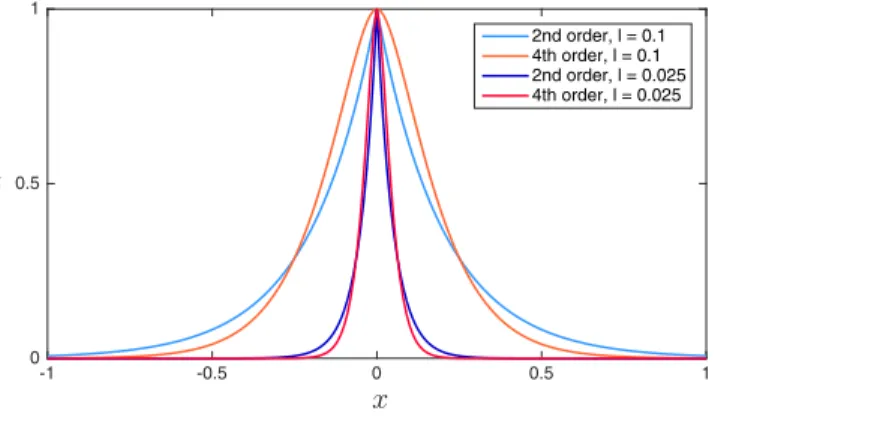
Fig. 1. Analytical solution of the second order phase-field s(x) = e−|x |2 l and fourth order phase-field s(x) = e −|x |
l (1 +|x |
l ) for different length
scale parameters.
where the value s = 0 refers to the undamaged and s = 1 to the fully broken material. The unknowns [ϕ, s] form a configuration space in Rn+1, representing the primal degrees of freedom to be found for all times of interest.
2.1. Regularised crack surface
Crack growth creates a new internal boundary Γ0cr(t) ⊂ Rn−1. Here, we assume that this process is based upon an energetic criterion. To be specific, the crack initiates or continues upon attainment of a critical local fracture energy density gc. Thus, the total energy within the sharp crack interface reads
Ecr =
Γcr 0
gcdΓ. (3)
Since the numerical evaluation of this sharp crack interface is not suitable within a standard finite element framework, a regularised crack interface using a specific regularisation profileγ (s) is introduced, such that the critical fracture energy is approximated byΓcr
0 gcdΓ ≈
B0gcγ (s) dV .
For the regularisation zone, a higher-order regularisation of the crack topology is utilised to obtain better accuracy and convergence rates of the numerical solution (see Borden et al. [14] for a detailed discussion). Therefore, we apply a fourth order approach for the crack-density functional
γ (s) = 1 4ls 2+ l 2∇(s) · ∇(s) + l3 4∆ 2(s). (4)
In Fig. 1 the analytical solution of the corresponding Euler equation of the fourth order approach in the one
dimensional case is compared to the solution of the Euler equation of the second order crack-density functional γ (s) = 1
2ls 2+ l
2∇(s) · ∇(s), see Miehe et al. [11] for details on the corresponding Euler equations.
2.2. Finite strain elasticity in a phase-field approach
For the non-linear mechanical field in a phase-field approach to fracture, we assume that the material behaviour is governed by a modified Helmholtz energy density function Ψ : B0×I → R, Ψ := Ψ (F, s) where F : B0×I → Rn×n
is the deformation gradient. Postulating that fracture requires a local state of tension, we define the fracture insensitive part of the deformation gradient as follows
˜ F = a (λ+ a)(1−s)(λ − a)na⊗Na, (5)
where na and Na denote the principal directions of the left and right stretch tensors. Moreover, λa are principal
Weinberg [13] for further details. Accordingly, we define the local constitutive relations P( ˜F(F, s)) = ∂Ψ( ˜F(F, s))
∂F , (6)
H( ˜F(F, s)) = ∂Ψ( ˜F(F, s))
∂s , (7)
where P : B0×I → Rn×nrepresents the first Piola–Kirchhoff stress tensor and H : B0×I → R the driving force
of the phase-field. The Lagrangian form of the local balance of linear momentum as well as of the phase-field balance equation1reads ρ0v = DIV(P) + ¯B,˙ (8) 0 = H + gc 2ls − gcl∆(s) + gcl3 2 ∆ 2(s). (9)
The external contributions at the boundary are specified by appropriate Dirichlet and Neumann boundary conditions on the mechanical and the phase-field, respectively
ϕ = ¯ϕ on ∂B0ϕ× [0, T ], s = ¯s on∂Bsd
0 × [0, T ],
PN = ¯T on∂B0σ× [0, T ], ∇(l3∆(s) − ls) · N = 0 on ∂Bsn
0 × [0, T ].
(10) An additional boundary contribution for the phase-field arises due to the structure of the fourth order approach, given as ∆(s) = 0 on ∂B0× [0, T ]. Note that we consider hereinafter only pure Neumann contributions on the whole
boundary∂B0, since Dirichlet boundaries are usually not defined for the phase-field. Finally, initial conditions for the
mechanical as well as for the phase-field are given as
ϕ(X, 0) = ϕ0, ϕ(X, 0) = v˙ 0, s(X, 0) = 0, in B0 (11)
which completes the coupled initial–boundary value problem (IBVP) under consideration. 2.3. Weak formulation
Next, the spaces of virtual or admissible test functions for the deformation as well as for the phase-field are introduced as follows
Vϕ = {δϕ ∈ H1(B0) | δϕ = 0 on ∂Bϕ
0}, (12)
Vs= {δs ∈ H2(B
0) | δs = 0 on Γ0cr}, (13)
where H denotes the Sobolev functional space of square integrable functions and derivatives. Note that the phase-field requires being in H2(B0), which has substantial effects for the numerical solution of the coupled IBVP using finite
elements. The weak form of the balance equation of the coupled phase-field approach to fracture reads Gϕ:= B0 ρ0δϕ · ¨ϕ + P : ∇X (δϕ) dV − B0 δϕ · ¯B dV − ∂Bσ 0 δϕ · ¯T dA = 0, (14) Gs:= B0 δsH +gc 2ls +gcl∇(δs) · ∇(s) + gcl3 2 ∆(δs)∆(s) dV = 0. (15)
Postulating that the coupled IBVP considered here obeys the fundamental first and second law of thermodynamics, we follow the lines of arguments outlined in Hesch and Weinberg [13] to demonstrate the validness of the considered approach. In a first step, the first law of thermodynamics is analysed for the system at hand, representing the global energy balance. To this end, suitable substitutions of the variationsδϕ = ˙ϕ are introduced in(14)such that
B0 ρ0 1 2 d dt( ˙ϕ · ˙ϕ) + P : ˙F dV = B0 ˙ ϕ · ¯B dV + ∂Bσ 0 ˙ ϕ · ¯T dA. (16)
1 Since the order parameter s is dimensionless, the corresponding balance equation can be regarded as a Ginzburg–Landau type evolution equation for the phase-field.
Since dtd(12B
0 ρ0( ˙ϕ · ˙ϕ) dV ) =
d
dtT, ˙Ψ( ˜F(F, s)) = P : ˙F + H˙s and the terms on the right hand side represent the
external power Pex t, we obtain d dtT + B0 ˙ Ψ( ˜F(F, s)) − H˙s dV = Pex t. (17) Substitutingδs = ˙s in(15)yields B0 ˙ sH + gc 2ls +gcl∇(˙s) · ∇(s) + gcl3 2 ∆(˙s)∆(s) dV = 0. (18)
Insertion of (4)and introducing the abbreviation DP F :=
B0gcγ dV for the global dissipation we finally end up˙
with d dtT + P
i nt+D
P F=Pex t. (19)
The last statement represents the global energy balance of the dissipative system.
Remark. Miehe et al. [1], demand ˙s ≥ 0, which is equivalent to ˙γ ≥ 0 since ∂Ψ∂s ≤ 0, for thermodynamical consistency, avoiding a transfer of energy from the phase into the mechanical field. This prevents healing effects, which may be taken into account as well. Here, we only restrict the fully broken state, i.e. we allow for healing until the phase-field reaches one.
2.4. Contact formulation
Assuming that multiple bodies i are in contact,2the boundary of the mechanical field requires further subdivision ∂B(i),c0 ∪∂B (i),ϕ 0 ∪∂B (i),σ 0 =∂B (i) 0 , (20) along with
∂B0(i),c∩∂B0(i),ϕ=∂B(i),c0 ∩∂B0(i),σ =∂B0(i),ϕ∩∂B0(i),σ = ∅. (21)
Note that the actual contact surface∂B0(i),c does not interfere with the phase field boundary, which is in contrast to, e.g., a thermal boundary of a thermomechanical problem which establishes an energy transfer across the contact zone. Taking the local linear momentum balance across the contact interface into account, the contact contributions to the total virtual work of a two body contact problem can be written as
Gc=
∂B0(1),c
t(1)·(δϕ(1)−δϕ(2)) dA, (22)
where t(1)denotes the Piola tractions related to the surface∂B0(1),c. Next, we decompose the contact tractions in normal and tangential components as
t(1)=tNν + tT, tT ·ν = 0, tT =tT,αaα. (23)
Here,ν denotes the current outward normal vector on ∂B0(1),cand aα,α ∈ [1, 2] the contravariant tangential basis vectors. For convenience, we introduce the gap functions in normal and tangential directions
gN=ν · (ϕ(1)−ϕ(2)), gT =(I − ν ⊗ ν) · (ϕ(1)−ϕ(2)). (24)
The normal contact conditions are given in the form of Karush–Kuhn–Tucker (KKT) conditions via
gN≤0, tN≥0, tNgN =0, (25)
which are the classical complementary condition for contact problems. Furthermore, we postulate that the frictional response is prescribed by Coulomb’s friction law, given as follows
ˆ φc:= ∥tT∥ −µ|tN| ≤0, ˙ ζ ≥ 0, ˆ φcζ = 0,˙ L tT =ϵT ˙ gsT − ˙ζ tT ∥tT∥ . (26)
The last equation makes use of the Lie derivativeL tT = ˙tT,αaα of the frictional tractions and aligns them to the
tangential velocity ˙gsT with respect to the tangential penalty parameterϵT. Note that the penalisation of the stick
condition implies an additive split of the tangential gap into a reversible (elastic) part geT and an irreversible (inelastic) part gsT. Moreover, µ denotes the coefficient of friction and ˙ζ a consistency parameter in analogy to the plastic multiplier in plasticity, where ˙ζ = 0 represents stick and ˙ζ > 0 slip.
To demonstrate thermodynamical consistency, we introduce a local energy density function Ψc := Ψc(ϕ) and
substitute againδϕ = ˙ϕ. The global power balance across the interface reads now ∂B0(1),c ˙ Ψc dV = ∂B(1),c0 tNg˙N+tT ·(˙geT + ˙gsT) dV. (27)
Enforcing(25)exactly and assuming that the elastic part of the tangential gap is small enough to be neglected, the global frictional dissipation is given by
Dc=
∂B(1),c0
tT · ˙gsT dV. (28)
Along with the dissipation of energy into the phase-field, the total dissipation is given by D = DP F+Dc. This total
dissipation D represents the amount of energy transferred into the thermal field, which we did not consider here. 3. Isogeometric discretisation and local refinement
Concerning the spatial discretisation, displacement based finite elements are applied. Accordingly, polynomial approximations of the deformation and its variations, written as
ϕh= A∈ω RAqA, δϕh= A∈ω RAδqA, (29)
are introduced, where RA : B0 → R are global shape functions associated with control points A ∈ ω =
{1, . . . , nnode}. For the phase-field and its variation we apply a discretisation conforming to the discretisation of
the deformation sh= A∈ω RAsA, δsh= A∈ω RAδsA. (30)
For the phase-field equation in(15), at least C1continuous shape functions are mandatory. To fulfil this requirement, we make use of quadratic NURBS shape functions
RA:=Rip,j,k,q,r(ξ) = Ni,p(ξ)Mj,q(η)Lk,r(ζ)wi,j,k n ˆi=1 m ˆj=1 l ˆk=1 Nˆi,p(ξ)Mˆj,q(η)Lˆk,r(ζ )wˆi,ˆj,ˆk , (31)
where n, m, l denote the number of control points along each parametric direction. In addition, p, q, r denotes the order of the non-rational B-Splines N , M and L along with the NURBS weightswˆi,ˆj,ˆk. For further details on the construction of B-Splines for finite element analysis, see Cottrell et al. [15].
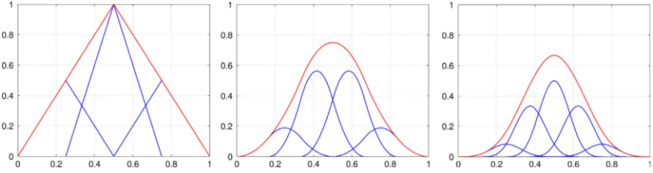
Fig. 2. Subdivision of 1D linear, quadratic and cubic B-splines.
3.1. Hierarchical B-spline and NURBS spaces
Classical refinement procedures rely on the subdivision of elements, which is not an applicable procedure for higher-order problems, since the classical approaches do not conserve the required higher continuity. To circumvent this issue, we focus on a subdivision of the basis functions themselves. This allows us to maintain the required continuity by replacing the underlying B-Splines using a linear combination of splines via
Bk,A=Bpk,i(ξ) = p+1 j=0 d l=1 2−pl pl+1 jl Nil,pl(2ξ l− j lhl−ξill), (32)
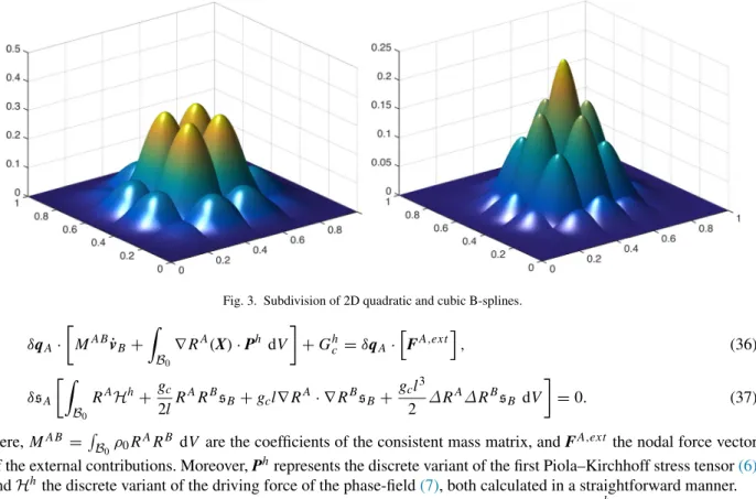
where hl refers to the coarse level element length in the parameter space. To visualise this refinement procedure, the
subdivision for one dimensional shape functions is shown inFig. 2, whereasFig. 3demonstrates the two dimensional case. Since the refined level consists of copied and scaled versions of the original B-Spline, further local refinements can be applied level by level. To rewrite this approach in a more convenient way, we introduce a subdivision matrix S (with components Si,j) providing the scaling information in(32)and obtain
Bpk,i(ξ) =
p+1
j=0
Si,jBpk+1,2i−1+j(ξ). (33)
Once the subdivision matrix is established, we recalculate the control mesh along with the associated primal variables for the deformation and the phase-field
qk+1A =STAqkA, sk+1A =STAskA, (34)
where STAaddresses a single row in the subdivision matrix corresponding to node A, i.e. qk+1A represents a set of new coordinates. The extension of B-Splines to NURBS as outlined in(31)is tedious, but straightforward
Rk,A=Rpk,i(ξ) = p+1 j=0 Si,jBpk+1,2i−1+j(ξ)wk+12i−1+j i p+1 j=0 Si,jBpk+1,2i−1+j(ξ)wk+12i−1+j . (35)
Note that (32) is only valid for uniform knot vectors and has to be modified for non-uniform knot vectors, see Sabin [31]. For further details, e.g. for the case of repeated knots, details on the construction of the subdivision matrix and its application to control points of NURBS instead of B-spline basis functions as well as the numerical evaluation of the finite elements, see Hesch et al. [24].
3.2. Semi discrete formulation of the coupled problem
Fig. 3. Subdivision of 2D quadratic and cubic B-splines. δqA· MA Bv˙B+ B0 ∇RA(X) · Ph dV +Ghc =δqA·FA,ext , (36) δsA B0 RAHh+gc 2lR ARBs B+gcl∇ RA· ∇RBsB+ gcl3 2 ∆R A∆RBs B dV =0. (37) Here, MA B =B 0ρ0R
ARB dV are the coefficients of the consistent mass matrix, and FA,extthe nodal force vector
of the external contributions. Moreover, Phrepresents the discrete variant of the first Piola–Kirchhoff stress tensor(6)
and Hhthe discrete variant of the driving force of the phase-field(7), both calculated in a straightforward manner. To complete the semi-discrete formulation, we define the discrete contact contributions Ghc. In particular, we aim at a Mortar based approach for the contact interface. Therefore, the space of admissible test functions for the discrete Lagrange multiplier field is introduced as
Mh= {δt(1),h∈L2(∂B(1),c
0 ∩∂B
(2),c
0 )}. (38)
For the ease of construction of the discrete Lagrange multiplier space, an approximation of linear order for the dual space has been introduced in Hesch and Betsch [32] for domain decomposition and in Dittmann et al. [25] for contact problems. This variant is efficient to implement and satisfies the necessary convergence order for the quadratic primal space we use to fulfil the C1 requirement of the coupled problem at hand, see Brivadis et al. [33] for detailed investigations on this topic. In particular, we utilise a set of nodes ˜ω(1) = [ ˜q1, . . . , ˜qnsurf]on the physical contact
boundary, where nsurfcorresponds to the number of physical nodes on the surface geometry of B(1)and obtain
t(1),h= A∈ ˜ω(1) NAλA, δt(1),h= A∈ ˜ω(1) NAδλA, (39) where NA:∂B(1),c
0 → R are (n − 1) dimensional shape functions associated with nodes A ∈ ˜ω(1).
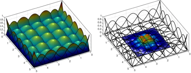
Note that the discrete Lagrange multiplier space has to be constructed with care to avoid possible singularities. To clarify this issue,Fig. 4shows a representative example for quadratic B-Splines. The unrefined situation is displayed on the left hand side, consisting of 49 shape functions on the particular surface with 36 possible nodes. On the right hand side, a single B-Spline has been refined (all remaining shape functions are transparent in this figure). Here, we obtain 64 shape functions with associated degrees of freedom, whereas 69 nodes on the surface are given.
Consideration of a low order Lagrange multiplier space, e.g., a Dirac distribution of the multipliers at the physical nodes would clearly overconstrain the system. This issue arises for constraints like Dirichlet boundary conditions or for incompressibility constraints. We did not observe this for the contact constraints, although this cannot be ruled out by design. A simple remedy can be considered: Since this issue arises only in the transfer area between coarse and fully refined mesh, the Lagrange multipliers can be placed on the coarse level elements, reducing the total number of constraints.
Fig. 4. Unrefined quadratic NURBS functions (left), refined shape function (right).
Once the approximation of the dual space is established, the construction of the Mortar contact constraints is straightforward. Decomposing again the tractionsλA into normalλN,A and tangentialλT,A components and
subse-quently inserting them in the contact contributions yields
Ghc =λN,Aν ·nA Bδq(1)B −nACδq(2)C +λT,A·(I − ν ⊗ ν)nA Bδq(1)B −nACδq(2)C , (40) where we make use of the well-known definition of Mortar integrals
nA B = ∂B(1),c0 NA(ξ(1))RB(ξ(1)) dA, nAC = ∂B(1),c0 NA(ξ(1))RC(ξ(2)) dA. (41)
The Mortar integrals must be carefully subdivided for the numerical evaluation such that each subdomain of integra-tion contains well-posed areas of both surfaces, i.e. segments are not allowed to cross element boundaries. Therefore, an isoparametric transformation using bilinear, triangular shape functions MK is introduced
ξ(i),h(η) =
3
K =1
MK(η)ξ(i)K, (42)
and we obtain the segment contributions nκβ = △ Nκ(ξ(1),h(η))Rβ(ξ(1),h(η))Jseg dη, nκζ = △ Nκ(ξ(1),h(η))Rζ(ξ(2),h(η))Jseg dη, (43)
which have to be assembled into the global system, see Hesch and Betsch [34,35] and the references therein. Moreover, the Jacobian of each segment is required
Jseg= ∥A1(ξ(1),h(η)) × A2(ξ(1),h(η))∥ det(Dξ(η)), (44)
where Aα(ξ) = R,αA(ξ)qAdenotes the tangential vectors in the reference configuration.
4. Temporal discretisation
For the temporal discretisation, we subdivide the time period I into a sequence of times t0, . . . , tn, tn+1, . . . , T
and assume that the state at tn, denoted by (qA,n, sA,n), is known. Then we approximate the state at tn+1 with
4.1. Full discrete formulation of the coupled problem
For the coupled system we obtain the solution of each time step by solving the algebraic equations δqA· 2 ∆tM A B(q B,n+1−qB,n−∆t vB,n) + B0 ∇RA(X) · Pnh,n+1 dV +Ghc,n,n+1=δqA· Fn+1A,ext/2 , (45) and δsA B0 RAHhn+1/2+gc 2lR ARBs B,n+1/2+gcl∇ RA· ∇RBsB,n+1/2 + gcl 3 2 ∆R A∆RBs B,n+1/2dV =0. (46)
Here,(•)n and(•)n+1 denote the value of a given physical quantity at time tn and tn+1, respectively. Moreover,
Phn,n+1 represents the usual mid-point evaluation of the first Piola–Kirchhoff stress tensor. A structure-preserving variant thereof based on a specific evaluation of the second Piola–Kirchhoff stress tensor is presented in Hesch and Weinberg [13]. This approach allows to conserve algorithmically both momentum maps as well as the total energy of the unconstrained system.
4.2. Full discrete formulation of the contact constraints
Consistent with the above given discretisation of the bulk, the temporal discretisation of the virtual work of the normal contact contributions is given by
Gϕ,hc,N =λN,A,n+1nn+1/2·
nnA Bδq(1)B −nnACδq(2)C , (47) whereas the tangential contact contributions read
Gϕ,hc,T =λT,A,n+1/2·(I − nn+1/2⊗nn+1/2)
nnA Bδq(1)B −nnACδq(2)C . (48) To determine the Coulomb frictional traction a return map strategy is applied
λtrial
T,A,n+1=λT,A,n+ϵT(I − nn+1/2⊗nn+1/2)(nn+1A B −nnA B)q(1)B,n+1/2−(n AC
n+1−nnAC)q(2)C,n+1/2 , (49)
where the slip function can be obtained for each node A separately ˆ
φc,A,n+1= ∥λtrialT,A,n+1∥ −µ|λN,A,n+1|. (50)
We finally obtain for the frictional tractions
λT,A,n+1= λtrial T,A,n+1, if ˆφc,A,n+1≤0, µ|λN,A,n+1| λtrial T,A,n+1
∥λtrialT,A,n+1∥, elseif ˆφc,A,n+1> 0.
(51)
Once the frictional tractions at time tn+1are calculated, the corresponding midpoint approximation reads
λT,A,n+1/2=
1
2(λT,A,n+1+λT,A,n), (52)
where we follow the arguments outlined in Armero and Pet¨ocz [36]. For the construction of energy–momentum schemes of Mortar contact constraints, acting on the mechanical field we refer to Hesch and Betsch [34].
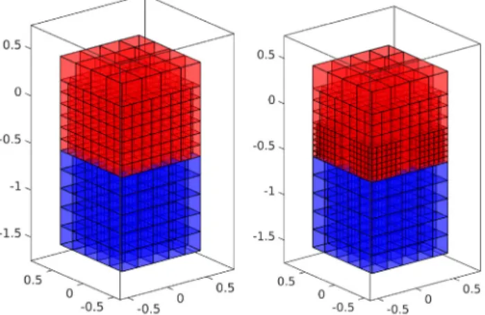
Fig. 5. Patch test: One level refinement (left) and one level refinement with additional two level refinement at the corners of the interface (right).
5. Numerical examples
In this section we evaluate the applicability and accuracy of the proposed methodologies within a three-dimensional environment. Hierarchical refinement procedures are tested for contact as well as for the phase-field approach to fracture. All algorithms are implemented for arbitrary NURBS basis functions, although we use weights equal to one if not otherwise stated. Moreover, refined areas are predefined a priori. Eventually, all presented procedures and methods are combined within a high velocity impact simulation.
5.1. Patch test
This numerical example is introduced to demonstrate the accuracy of the Mortar method in conjunction with hierarchical refinements. Therefore, we investigate two non conform meshed blocks with hierarchical refinements on the upper side of the contact interface, seeFig. 5for details of the geometry. The upper block consists of 4 × 4 × 4 elements whereas the lower block consists of 5 × 5 × 5 elements on level 0.
All elements on the lower plane of the upper block have been refined, seeFig. 5, left hand side. Moreover, a two level hierarchical refinement has been applied to the corner nodes of this plane, seeFig. 5, right hand side. For the one level refinement we obtain 400 + 125 elements and overall 3477 degrees of freedom, whereas we obtain for the two level refinement in total 1156 + 125 elements and overall 6069 degrees of freedom. Due to the support of the applied quadratic shape functions, large areas between coarse and fully refined elements arise within the contact boundary.
A Neumann boundary is applied to the top surface of the upper block, whereas the lower block is clamped, such that the body can expand in tangential direction. The constitutive behaviour is governed by a compressible Neo-Hooke material with associated strain energy density function given by
Ψ(i)(C(i)) = µ (i) 2 tr(C(i)) − n+λ 2 (ln(J)) 2−µ ln(J), (53)
where the Lam´e parameters are assumed to take the valuesλ = 1298.1 and µ = 865.3846, which corresponds to a Young’s modulus of E = 2250 and a Poisson ratio of 0.3. The density of both bodies is neglected for this quasi-static setup.
The von Mises stress results are shown inFig. 6for a uniform and constant pressure field ofσ = −2e3 applied to the upper Neumann boundary. As can be seen, the solution shows a nearly perfect constant pressure field across the interface, independent of the application of local, hierarchical refinements.
5.2. Ironing
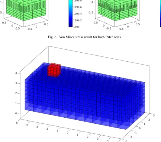
This next example demonstrates the applicability of hierarchical refinement to Mortar based frictional contact, using a setup similar to the ironing problem in Puso and Laursen [37].Fig. 7shows the reference configuration of this problem. The upper block of size 0.9 × 0.9 × 0.9 consists of 27 quadratic NURBS elements and the lower block
Fig. 6. Von Mises stress result for both Patch tests.
Fig. 7. Frictional ironing: Reference configuration.
of size 10 × 4 × 3 consists of 12 × 5 × 4 quadratic NURBS elements on level 0. Moreover, a two level hierarchical refinement is applied to the lower block, such that we obtain overall 5196 + 27 elements with together 14,037 degrees of freedom.
The material behaviour is again governed by a Neo-Hookean model with Lam´e parametersλ = 7500/13 and µ = 5000/13 for the upper block and λ = 75/13 and µ = 50/13 for the lower block. This values correspond to a Young’s modulus of E = 1000 and E = 10, respectively and to a Poisson’s ratio ofν = 0.3 for both blocks.
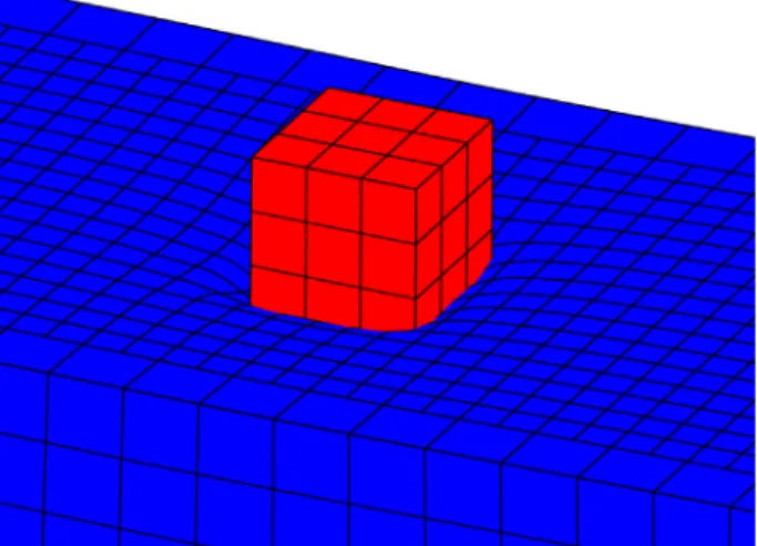
The top surface of the upper block moves −0.3 in vertical direction, afterwards 6 in horizontal direction and finally again 0.6 in vertical direction, whereas the bottom surface of the lower block is fixed in all directions. For each vertical movement 10 quasi-static time steps are applied and 200 quasi-static timesteps for the horizontal movement. The configuration at time t = 0.5 is depicted inFig. 8using a friction coefficient ofµ = 0.2.
In total 16 Lagrange multipliers are used, located at the lower surface of the upper block. InFig. 9, the resultant total forces at the top surface of the upper block in x, y and z direction are displayed. As can be seen, the proposed Mortar approach for hierarchical refined NURBS facilitates very good results for this relatively coarse mesh. For comparison, we added results for a nodal wise KTS-like approach, see Matzen et al. [38]. We placed the Lagrange multiplier on the upper surface of the lower block, since the application to the lower surface of the upper block yields
Fig. 8. Frictional ironing: Deformed configuration at time t = 0.5.
Fig. 9. Applied forces over time for a friction coefficientµ = 0.2.
Fig. 10. Bending contact fracture problem with reference configuration (upper).
unphysical deformations at the lower surface, such that we could not obtain any useful results. As clearly demonstrated
inFig. 9, nodal wise approaches suffer from heavy oscillations even with almost twice as much contact constraints.
5.3. Bending fracture problem
The purpose of this example is to demonstrate the capabilities of the phase-field approach within a contact situation. In particular, we consider a deformable block to be in contact with an elastic plate, see Fig. 10 for the initial configuration. The plate is clamped and locally refined using a three level hierarchical refinement on the right hand side, since we expect peak stresses within this area. Moreover, the contact area is locally refined as well.
The plate is of size 20 × 30 × 2 with centre point placed at [0, 15, 1], whereas the block is of size 4 × 4 × 4 with centre point placed at [0, 26, 4.5]. For both bodies, we assume again that the constitutive behaviour is governed by the
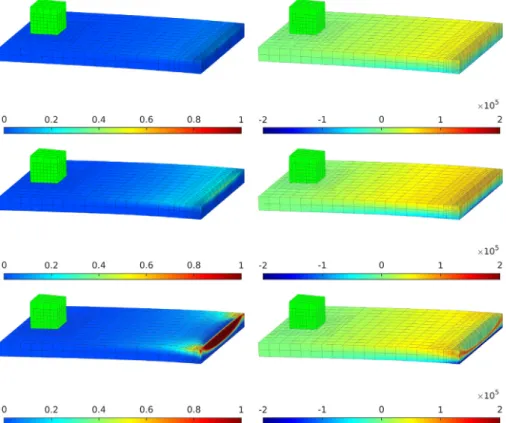
Fig. 11. Bending contact fracture problem, phase-field after 300, 500 and 582 steps (from top to down, left) andσ22stress distribution (right).
Neo-Hooke material law given in(53). The Lam´e parameters of the plate are assumed to take the valuesλ = 1.1538e7 andµ = 7.6923e6, which corresponds to a Young’s modulus of E = 2e7 and a Poisson ratio of 0.3. Moreover, the Lam´e parameters of the block are given byλ = 2.8846e4 and µ = 1.9231e4, which corresponds to a Young’s modulus of E = 5e4 and a Poisson ratio of 0.3. The phase-field parameters for the plate are chosen as gc=2.7 × 10²
and l = 0.1538.
Moreover the upper boundary of the block is moved downwards with a constant increment size of ∆u = 5 × 10⁻³ in e3direction for the first 200 steps and ∆u = 2.5 × 10⁻³for the remaining steps. The block consists of 4 × 4 × 4
elements and the plate of 13 × 19 × 2 elements on level 0. A local refinement is applied to the block as well as the expected contact area on the plate using a one level refinement. Furthermore, a three level refinement is applied to the Dirichlet boundary. In total 12,948 elements with overall 72,912 degrees of freedom are used and we obtain a minimal element size of hmin=0.0769, i.e. nearly half the size of the length parameter of the phase-field. Note that a globally
refined plate would require more than three million degrees of freedom without improvements on the accuracy of the areas of interest.
The phase-field as well as theσ22 stress distribution is depicted inFig. 11 for different load steps. As can be
observed the plate is nearly completely ripped out of the bearing. We stopped the simulation at this point, since the plate simply becomes statically undetermined. The associated load-deflection curve is given inFig. 12.
5.4. Impact problem
In this final example we consider a transient impact problem in conjunction with the proposed phase-field approach to fracture, seeFig. 13for the reference configuration of the bodies in contact. The initial velocity of the upper, wedge-shaped body is v = [0 0 − 100] m/s, whereas the long edges of the plate are fixed in space. The wedge-shaped body is approximately of dimension 0.2 m × 0.05 m × 0.134 m and consists of 24 × 6 × 12 quadratic NURBS elements on level 0. A one level hierarchical refinement is applied to the lower elements to refine the sharp-edged contact surface. The plate of size 0.36 m × 0.18 m × 0.018 m consists of 40 × 20 × 2 quadratic NURBS elements on level 0. A two level hierarchical refinement is used to achieve a sufficient mesh resolution of the possible impact region. The plate
Fig. 12. Bending fracture problem, load-deflection curve.
Fig. 13. Impact: Reference configuration.
is equipped with the presented phase-field approach to fracture, thus we obtain in total 27,632 elements and 100,760 degrees of freedom.
The material behaviour of both bodies is governed by a Neo-Hookean model, where the Lam´e parameters of the wedge-shaped body correspond to steel-like material and take the valuesλ = 121.15 GPa and µ = 80.77 GPa. In addition the mass density isρ = 7850 kg/m3. For the plate we apply a synthetic substance with Lam´e parameters λ = 0.208 GPa and µ = 0.073 GPa and a mass density ρ = 1070 kg/m3. Moreover, the phase-field parameters are
set to gc=350 N/m and l = 4.5 × 10⁻³m.
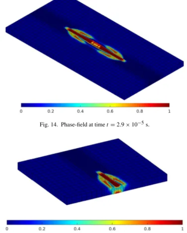
InFig. 14the phase-field is shown for the plate after 145 constant timesteps of size 2 × 10⁻⁷s. A sectional view
of the plate is given inFig. 15, whereas a detailed snapshot of the crack progression is shown inFig. 16. The latter figure displays the isosurface for s = 0.7 within the body. We can see that the surface in contact itself fractures with additional fracturing of the same surface parallel to the impact region. Moreover, due to bending of the lower surface additional cracks are initialised at the bottom of the plate as well and the crack fronts are merging within the plate.
This last example demonstrates the capabilities of the proposed phase-field methodology to deal with complex three dimensional crack patterns within an impact situation.
6. Conclusions
In this paper, contact formulations within the context of isogeometric analysis are adapted to the field of fracture mechanics. To ensure sufficient accuracy of the chosen phase-field approach, a fourth order crack-density functional is introduced, requiring at least C1continuity within the domain. This issue could be resolved easily with the proposed isogeometrical Mortar contact framework, demonstrating the generality and flexibility of the proposed approach.
Fig. 14. Phase-field at time t = 2.9 × 10⁻⁵s.
Fig. 15. Sectional view of plate at position x = 0.153, phase-field at time t = 2.9 × 10⁻⁵s.
Fig. 16. Three dimensional crack propagation at time t = 2.9 × 10⁻⁵s, displaying the isosurface for s = 0.7.
To resolve local features, in particular predefined contact as well as fractured areas, hierarchical refinement schemes are applied. They preserve the required continuity and reduce the computational costs for the three dimensional simu-lations dramatically, since standard NURBS discretisations only allow for global refinement. Moreover, the proposed hierarchical refinement schemes are combined for the first time with Mortar contact formulations within a three di-mensional framework. The chosen multiplicative decomposition of the deformation gradient into a compressive and a tensile part allows for the extension of the phase-field formulation to a large deformation setting which is inevitable in transient contact simulations with large displacements.
Acknowledgements
Support for this research was provided by the Deutsche Forschungsgemeinschaft (DFG) under grant HE5943/3-2, HE5943/5-1 and HE5943/6-1. This support is gratefully acknowledged.
References
[1] C. Miehe, M. Hofacker, F. Welschinger, A phase field model for rate-independent crack propagation: Robust algorithmic implementation based on operator splits, Comput. Methods Appl. Mech. Engrg. 199 (2010) 2765–2778.
[2] C. Miehe, F. Welschinger, M. Hofacker, Thermodynamically consistent phase-field models of fracture: Variational principles and multi-field FE implementations, Internat. J. Numer. Methods Engrg. 83 (2010) 1273–1311.
[3] C. Kuhn, R. M¨uller, A continuum phase field model for fracture, Eng. Fract. Mech. 77 (2010) 3625–3634.
[4] K. Weinberg, C. Hesch, A high-order finite-deformation phase-field approach to fracture, Contin. Mech. Thermodyn. (2015)http://dx.doi.org/ 10.1007/s00161-015-0440-7.
[5] G.A. Francfort, J.-J. Marigo, Revisiting brittle fracture as an energy minimization problem, J. Mech. Phys. Solids 46 (1998) 1319–1342.
[6] B. Bourdin, G.A. Francfort, J.J. Marigo, The variational approach to fracture, J. Elasticity 9 (2008) 5–148.
[7] A. Karma, D.A. Kessler, H. Levine, Phase-field model of mode III dynamic fracture, Phys. Rev. Lett. 81 (2001) 045501.
[8] V. Hakim, A. Karma, Laws of crack motion and phase-field models of fracture, J. Mech. Phys. Solids 57 (2009) 342–368.
[9] H. Henry, H. Levine, Dynamic instabilities of fracture under biaxial strain using a phase field model, Phys. Rev. Lett. 93 (2004) 105505.
[10] H. Henry, Study of the branching instability using a phase field model of inplane crack propagation, Europhys. Lett. 83 (2008) 16004.
[11] C. Miehe, L.M. Sch¨anzel, H. Ulmer, Phase field modeling of fracture in multi-physics problems. Part I. Balance of crack surface and failure criteria for brittle crack propagation in thermo-elastic solids, Comput. Methods Appl. Mech. Engrg. 294 (2015) 449–485.
[12] C.V. Verhoosel, R. de Borst, A phase-field model for cohesive fracture, Internat. J. Numer. Methods Engrg. 96 (2013) 43–62.
[13] C. Hesch, K. Weinberg, Thermodynamically consistent algorithms for a finite-deformation phase-field approach to fracture, Internat. J. Numer. Methods Engrg. 99 (2014) 906–924.
[14] M.J. Borden, T.J.R. Hughes, C.M. Landis, C.V. Verhoosel, A higher-order phase-field model for brittle fracture: Formulation and analysis within the isogeometric analysis framework, Comput. Methods Appl. Mech. Engrg. 273 (2014) 100–118.
[15] J.A. Cottrell, T.J.R. Hughes, Y. Bazilevs, Isogeometric Analysis: Toward Integration of CAD and FEA, Wiley, New York, 2009.
[16] Y. Bazilevs, V.M. Calo, J.A. Cottrell, J.A. Evans, T.J.R. Hughes, S. Lipton, M.A. Scott, T.W. Sederberg, Isogeometric analysis using T-splines, Comput. Methods Appl. Mech. Engrg. 199 (2010) 229–263.
[17] E.J. Evans, M.A. Scott, X. Lic, D.C. Thomas, Hierarchical T-splines: Analysis-suitability, B´ezier extraction, and application as an adaptive basis for isogeometric analysis, Comput. Methods Appl. Mech. Engrg. 284 (2015) 1–20.
[18] A.-V. Vuong, C. Giannelli, B. J¨uttler, B. Simeon, A hierarchical approach to adaptive local refinement in isogeometric analysis, Comput. Methods Appl. Mech. Engrg. 200 (2011) 3554–3567.
[19] D. Forsey, R.H. Bartels, Hierarchical B-spline refinement, Comput. Graph. 22 (1988) 205–212.
[20] D. Schillinger, L. Dede, M.A. Scott, J.A. Evans, M.J. Borden, E. Rank, T.J.R. Hughes, An isogeometric design–through–analysis methodology based on adaptive hierarchical refinement of NURBS, immersed boundary methods, and T-spline CAD surfaces, Comput. Methods Appl. Mech. Engrg. 249–252 (2012) 116–150.
[21] P.B. Bornemann, F. Cirak, A subdivision-based implementation of the hierarchical b-spline finite element method, Comput. Methods Appl. Mech. Engrg. 253 (2013) 584–598.
[22] M.J. Borden, C.V. Verhoosel, M.A. Scott, T.J.R. Hughes, C.M. Landis, A phase-field description of dynamic brittle fracture, Comput. Methods Appl. Mech. Engrg. 217–220 (2012) 77–95.
[23] W. Jiang, J.E. Dolbow, Adaptive refinement of hierarchical B-spline finite elements with an efficient data transfer algorithm, Internat. J. Numer. Methods Engrg. (2014).
[24] C. Hesch, S. Schuß, M. Dittmann, M. Franke, K. Weinberg, Isogeometric analysis and hierarchical refinement for higher-order phase-field models, Comput. Methods Appl. Mech. Engrg. (2015) submitted for publication.
[25] M. Dittmann, M. Franke, I. Temizer, C. Hesch, Isogeometric analysis and thermomechanical Mortar contact problems, Comput. Methods Appl. Mech. Engrg. 274 (2014) 192–212.
[26] L.D. Lorenzis, P. Wriggers, G. Zavarise, A mortar formulation for 3D large deformation contact using NURBS-based isogeometric analysis and the augmented Lagrangian method, Comput. Mech. (2012).
[27] R. Dimitri, L.D. Lorenzis, M.A. Scott, P. Wriggers, R.L. Taylor, G. Zavarise, Isogeometric large deformation frictionless contact using T-splines, Comput. Methods Appl. Mech. Engrg. 269 (2014) 394–414.
[28] I. Temizer, P. Wriggers, T.J.R. Hughes, Three-dimensional mortar-based frictional contact treatment in isogeometric analysis with NURBS, Comput. Methods Appl. Mech. Engrg. 209–212 (2012) 115–128.
[29] I. Temizer, Multiscale thermomechanical contact: Computational homogenization with isogeometric analysis, Internat. J. Numer. Methods Engrg. 97 (2014) 582–607.
[30] I. Temizer, C. Hesch, Hierarchical NURBS in frictionless contact, Comput. Methods Appl. Mech. Engrg. 299 (2016) 161–186.
[31] M. Sabin (Ed.), Analysis and Design of Univariate Subdivision Schemes, Springer, Heidelberg, 2010.
[32] C. Hesch, P. Betsch, Isogeometric analysis and domain decomposition methods, Comput. Methods Appl. Mech. Engrg. 213 (2012) 104–112.
[33] E. Brivadis, A. Buffa, B.I. Wohlmuth, L. Wunderlich, Isogeometric mortar methods, Comput. Methods Appl. Mech. Engrg. 284 (2015) 292–319.
[34] C. Hesch, P. Betsch, Transient 3D Domain Decomposition Problems: Frame-indifferent mortar constraints and conserving integration, Internat. J. Numer. Methods Engrg. 82 (2010) 329–358.
[35] C. Hesch, P. Betsch, Transient three-dimensional contact problems: mortar method. Mixed methods and conserving integration, Comput. Mech. 48 (2011) 461–475.
[36] F. Armero, E. Pet¨ocz, A new dissipative time-stepping algorithm for frictional contact problems: formulation and analysis, Comput. Methods Appl. Mech. Engrg. 179 (1999) 159–178.
[37] M.A. Puso, T.A. Laursen, A mortar segment-to-segment frictional contact method for large deformations, Comput. Methods Appl. Mech. Engrg. 193 (2004) 4891–4913.
[38] M.E. Matzen, T. Cichosz, M. Bischoff, A point to segment contact formulation for isogeometric, NURBS based finite elements, Comput. Methods Appl. Mech. Engrg. 255 (2013) 27–39.