Comput. Methods Appl. Mech. Engrg. 299 (2016) 161–186
www.elsevier.com/locate/cma
Hierarchical NURBS in frictionless contact
˙I. Temizer
a,∗, C. Hesch
baDepartment of Mechanical Engineering, Bilkent University, 06800 Ankara, Turkey
bInstitute of Mechanics, Karlsruhe Institute of Technology, Otto-Ammann-Platz 9, Karlsruhe 76131, Germany
Received 9 June 2015; received in revised form 24 October 2015; accepted 2 November 2015 Available online 11 November 2015
Highlights
• Novel isogeometric contact algorithms are introduced based on hierarchical NURBS. • Hierarchical mortar discretizations are derived for frictionless contact.
• The partition of unity property is explored for the construction of the mortar basis. • Exterior and interior point methods are applied in regularized and exact settings. • Full or lumped recovery approach is employed to define the kinematic mortar variable. Abstract
This work investigates mortar-based frictionless contact in the context of NURBS discretizations that are subjected to local hierarchical refinement. The investigations emphasize three sets of choices which lead to different contact algorithms that have distinct advantages and disadvantages. First, on the optimization side, both exterior and interior point methods are applied, thus spanning inexact constraint enforcement algorithms of the penalty or barrier type as well as exact ones of the primal–dual type. Second, on the discretization side, the hierarchical basis set of the mortar variables is inherited either directly from the discretization of the slave surface or after an intermediate normalization step to satisfy the partition of unity. Third, in interaction with both optimization and discretization, the kinematic mortar variable is recovered from the actual normal gap through the full or lumped solution of a linear system of equations. The implications of different choices are highlighted through benchmark problems which monitor the solution quality at the global level through the structural force evolution and at the local level through the contact pressure distribution.
c
⃝2015 Elsevier B.V. All rights reserved.
Keywords:Contact; Isogeometric analysis; Hierarchical refinement; Mortar method
1. Introduction
Contact interfaces are often small in size in comparison to representative structural dimensions yet their modeling requires highly efficient and robust schemes for a reliable prediction of phenomena which are driven by the
∗Corresponding author. Tel.: +90 312 290 3064.
E-mail address:[email protected](˙I. Temizer).
http://dx.doi.org/10.1016/j.cma.2015.11.006
contact conditions. The present work addresses the treatment of contact in the context of isogeometric analysis. Specifically, the aim is to explore the efficiency aspect by applying hierarchical discretization schemes that can concentrate the degrees of freedom within a zone of interest at the contact interface. Complementary investigations will additionally explore the robustness aspect by applying different optimization algorithms in the context of mortar-based discretizations.
Isogeometric analysis [1] has been established as a computational approach that has both enabling and facilitating features, for instance by allowing a direct transition from design to analysis and thereby circumventing the additional meshing stage. Contact mechanics particularly benefits from the intrinsic higher-order smoothness of isogeometric discretizations and from the underlying non-negative basis functions [2]. Almost all the studies on isogeometric contact to date have employed non-uniform rational B-splines (NURBS), mostly in a purely mechanical setting and often without friction. Among the first two studies, three-dimensional frictionless contact was studied in [3] using the penalty method together with a stable contact discretization that was developed for standard finite element discretizations [4,5]. In [6], the penalty method was used together with an intrinsically unstable Gauss-point-to-surface algorithm to investigate frictionless thermomechanical contact problems in a three-dimensional setting. Additionally, to recover stability, a NURBS-based discretization of the contact pressure was introduced in the spirit of the mortar method for two-dimensional linear elasticity. The two-dimensional extension of this mortar approach to incorporate friction was carried out using the penalty method in [7] and a three-dimensional extension was discussed in [8] where Uzawa augmentations were applied to improve the robustness of penalty regularization for both normal and tangential contact constraints. A two-dimensional mortar-based discretization scheme employing the Lagrange multiplier method, which ensures an exact enforcement of the contact constraints, was investigated in [9] in the absence friction and a three-dimensional Lagrange multiplier approach was presented in [10] within a frictional thermomechanical framework. An alternative approach to enforcing the constraints exactly is the augmented Lagrangian method [11] which was applied in a three-dimensional mortar-based frictionless setting in [12] and together with thermal contact constraints in [13]. While the formulation of [14,15] that was originally introduced for linear Lagrange discretizations is a common basis for mortar-based isogeometric contact discretizations, stable collocation-point-to-surface approaches have also been initiated in a two-dimensional frictionless setting [16].
From an optimization point of view, these studies exclusively employ exterior point methods such as the penalty, Lagrange multiplier and augmented Lagrangian methods. Recently, interior point methods [17] have also been applied to two- and three-dimensional mortar-based frictionless contact [18]. On the other hand, from a discretization point of view, all of these approaches are based on a Galerkin setting which introduces a weak form. An approach which takes the strong form as the starting point has also been introduced in a two-dimensional frictionless setting [19] based on isogeometric collocation [20].
The list of works reviewed above is not complete. In particular, applications to interface problems which benefit from similar algorithmic procedures were not mentioned, notably domain decomposition [21,22] and cohesive zones [23,24]. Similarly, no attempt is made to review the vast literature on which these studies are based with respect to the formulation and enforcement of the contact constraints as well as with respect to the description and discretization of the contact interface. The reader is referred to the cited works for specific references as well as to [25–27] for broad overviews.
The standard NURBS discretizations that have predominantly been employed in the reviewed studies only allow a global refinement of the basis structure. Among various possibilities, two widely adopted approaches enable local refinement in isogeometric analysis. One of these is T-splines [28,29]—see [30] for recent developments together with a refinement algorithm. In contact mechanics, T-splines have so far been applied only in a frictionless setting using the penalty method together within a Gauss-point-to-surface framework [31]. A major advantage with the T-spline approach is its ability to address complex topologies. Originally, T-T-splines were defined for bicubic surfaces [32]. However, the difficulty of constructing complex three-dimensional T-spline discretizations [33] with arbitrary orders [29] have recently been addressed. Another local refinement scheme is based on hierarchical refinement, start-ing with the approach of [34] that is applicable to both B-splines and NURBS, which has not been applied to contact problems so far and thus constitutes the focus of the present study. In [35], the approach in [34] has been extended to an adaptive framework which additionally ensures that the hierarchical basis satisfies the partition of unity. While these hierarchical refinement schemes can easily adopt arbitrary discretization orders, they are typically limited to a quadrilateral or hexahedral topology due to the underlying tensor-product structure. Recently, it has also become pos-sible to overcome this restriction [36]. In some sense, ideas from T-splines and hierarchical representations may also
be adopted, particularly in view of its algorithmic simplicity. Instead of addressing the lack of partition of unity prop-erty as in [35], its implications will first be discussed and then a straightforward normalization procedure is adopted to recover this property—see also [38] for an alternative scheme that satisfies the partition of unity by construction. Despite the special choice of the hierarchical refinement scheme, the addressed issues span a broad range of numerical concerns such that the developed contact algorithms would be beneficial for alternative refinement schemes as well.
The outline of this work is as follows. In Section 2, the hierarchical refinement scheme is described and demonstrated for bulk discretizations that automatically induce hierarchical discretizations on potential contact surfaces. The contact algorithm to be employed on such hierarchically refined surfaces is discussed in Section3, with a particular focus on the choice of the mortar basis as well as its use in describing and enforcing the contact constraints. Extensive numerical investigations will be presented in Section4 which range from classical benchmark examples with stationary contact interfaces, aiming to demonstrate fundamental features of various algorithmic choices, to more advanced tests with large sliding contact that focus on robustness and efficiency. Suggestions for possible future extensions and applications will be summarized in Section5.
2. Hierarchical refinement
The process of hierarchical refinement adopted in this work has three major stages: (i) the construction of the initial coarse level geometry description, (ii) the generation of a series of fine level descriptions, and (iii) the selection of basis functions from each level. The first two stages are standard procedures in isogeometric analysis and therefore are only briefly reviewed. The last stage which generates the hierarchical basis set is addressed in detail.
2.1. Reference geometry
In order to define the univariate B-spline functions associated with the i th dimension of a patch, an open knot vector Ξi,0 = {ξi,0 0 , . . . , ξ i,0 pi , ξ i,0 pi+1, . . . , ξ i,0 ni0, ξ i,0 n0i+1, . . . , ξ i,0 n0i+pi+1 } (2.1)
is assumed where pi is the polynomial order of the functions and n0i +1 would indicate the number of control points
in a one-dimensional setting. In a multi-dimensional setting, let X indicate the position vector associated with the referential geometry that is described using n0X control points X0I with corresponding weightsα0I. If the product of the univariate B-spline functions associated with a control point is denoted by B0I(ξ1, ξ2, ξ3), where ξispan the knot vectors, then the NURBS basis functions are defined by
N0I = α I 0B0I n0X J =1 αJ 0B J 0 (2.2)
such that the referential geometry admits the coarse level description
X = n0 X I =1 N0IX0I. (2.3)
2.2. Fine level descriptions
Starting with the coarse level description, a hierarchy of fine level descriptions may be built as follows. Let Ξi,0 = {ξi,0 0 , ξ i,0 1 , . . . , ξ i,0 mi0−1, ξ i,0 m0i} (2.4)
denote a modified vector which involves only unique knot entries. Here, m0i indicates the number of unique knot spans. In a non-hierarchical setting, these would help construct the isogeometric elements that serve as convenient
domains of integration for evaluating the weak form, their number equal to the product m0=Πim0i. The next level in
the hierarchy is constructed through knot refinement, specifically by halving the unique knot spans: Ξi,1= ξi,10 =ξ i,0 0 , ξ i,1 1 = 1 2(ξ i,0 0 +ξ i,0 1 ), . . . , ξ i,1 m1 i−1 = 1 2(ξ i,0 m0 i−1 +ξi,0 m0 i), ξ i,1 m1 i =ξi,0 m0 i . (2.5)
This leads to a new set of weightsα1J and control points X1I, computed using standard knot refinement algorithms [39], which are associated with m1 = Πimi1elements where m1i = 2m0i. Consequently, the geometry is preserved
but it admits the finer discretization X = n1X
I =1N1IX1I. By repeating this process through L levels one obtains an
embedded hierarchy of levels, each levelℓ ∈ [1, L] offering a larger number of degrees of freedom to describe the same reference geometry:
X =
nℓX
I =1
NℓIXℓI. (2.6)
2.3. Hierarchical basis functions
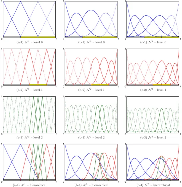
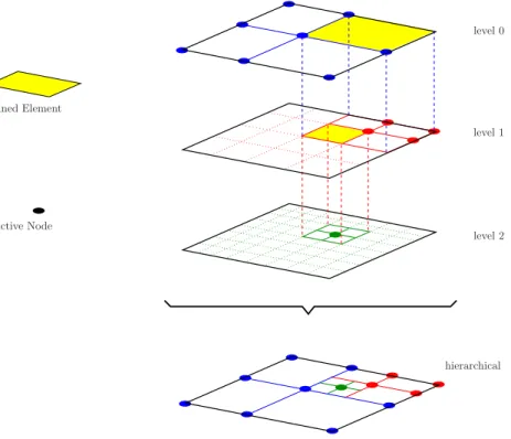
Hierarchical refinement will be triggered element-wise [34]. At levelℓ, let SℓI denote the span of a basis function NℓI and Rℓ ⊆ [0, 1] × [0, 1] × [0, 1] denote the span of all elements which are marked for hierarchical refinement such that Rℓ+1⊆Rℓ. The algorithm for selecting basis functions from each level in order to create a hierarchical set of basis functions is demonstrated inFig. 1and can be summarized as follows:
• STEP1 (Coarse Level): All coarse level basis functions are activated initially. Setℓ = 0. • STEP2 (Basis Deactivation): Deactivate all NℓIwith SℓI ⊆Rℓ.
• STEP3 (Basis Activation): Activate all Nℓ+1I with Sℓ+1I ⊆Rℓ.
• STEP4 (Level Loop): Setℓ = ℓ + 1 and continue with STEP2 until all levels are checked.
The remaining nuactive basis functions will be indicated by NI. These remaining functions are linearly independent
and cover the whole patch while concentrating the degrees of freedom around the selected regions of refinement. Denoting the displacement vector by u such that the current position vector is x = X + u, a subparametric hierarchical discretization can now be invoked [38]:
u =
nu
I =1
NIuI. (2.7)
The geometry is still described (exactly) by the initial coarse level discretization(2.3). Note that this initial discretiza-tion, and hence the ensuing hierarchical descripdiscretiza-tion, can employ different orders along each parametric direction.
The demonstration inFig. 1incorporates major aspects of the algorithm. Tracing the steps for the particular case of N1as an example, initially all basis functions at level 0 are active. Subsequently, two of these are removed since they
entirely lie in the zone of refinement towards level 1. Four basis functions from level 1 which lie within this zone are then activated. However, one is subsequently removed since it lies in the zone of refinement towards level 2. Within this zone, three basis functions from level 2 are activated, overall leading to a hierarchical discretization with eight basis functions. For the cases of N2and N3, one obtains nine basis functions. It is noted that the knot structure of the hierarchical basis inFig. 1as well as in similar subsequent figures solely serves a graphical purpose as an indication of the refinement process and does not directly induce the corresponding basis. This is evident for the case of N3 where there are nine basis functions although the knot structure can accommodate ten. In two and three dimensions, since there is no tensor product structure in a hierarchical setting, a maximum number of basis functions that can be accommodated cannot be deduced from the knot structure.
Due to the increasing span of the basis functions, the number of basis functions activated at each refinement step has a decreasing tendency when the order increases (see level 2 inFig. 1from N1to N3). The number of deactivated basis functions also decreases. In fact, the refinement of an element at a given level may not lead to the deactivation of basis functions at all (e.g. level 1 to level 2 inFig. 1for N2 and N3). However, overall, starting with the same number of elements at each order, the percentage increase in the number of basis functions in the transition from
Fig. 1. The hierarchical refinement algorithm is demonstrated. The refined elements are marked with yellow and the inactive basis functions at each level are indicated with dashed lines. Here and in upcoming discussions, the notation Nprefers to NURBS basis functions which emanate from B-splines of order p. (For interpretation of the references to colour in this figure legend, the reader is referred to the web version of this article.)
the coarse level basis set to the hierarchical one tends to decrease with increasing order. Consequently, in order to obtain a comparable increase in the numerical resolution, additional elements should be refined around the elements which indicate need for refinement. In general, the decision for hierarchical refinement may be driven through an error measure [37,36]. However, such adaptive schemes are outside the scope of the present work. Hence, in the numerical investigations, only pre-selected refinements will be employed in order to concentrate on the investigation of contact algorithms in a hierarchical setting.
The summarized hierarchical refinement strategy is reminiscent of the hanging nodes approach when first order elements are used, as depicted inFig. 2. Indeed, there are qualitative similarities, e.g. the integration of the finite element weak form will be carried out using the hierarchical element set. Referring toFig. 2, these are the four level 2 elements, followed by the three non-refined level 1 elements and the three level 0 elements. However, an important difference of the present hierarchical refinement algorithm from the classical hanging node approach is that the basis function activation/deactivation is not carried out locally within each element but rather globally across the whole mesh. For instance, inFig. 2, the shape function of the central node from level 0 is active not only within the non-refined level 0 elements but across the whole domain. As a consequence, although the classical hanging nodes
Fig. 2. The hierarchical refinement strategy is depicted with first order (Lagrange or NURBS) elements. The global shape functions which are active are indicated by their corresponding nodes. The resulting hierarchical set of elements contains four level 2, three level 1 and three level 0 elements.
approach leads to a basis which satisfies the partition of unity the present hierarchical refinement algorithm does not—see Section3.2.
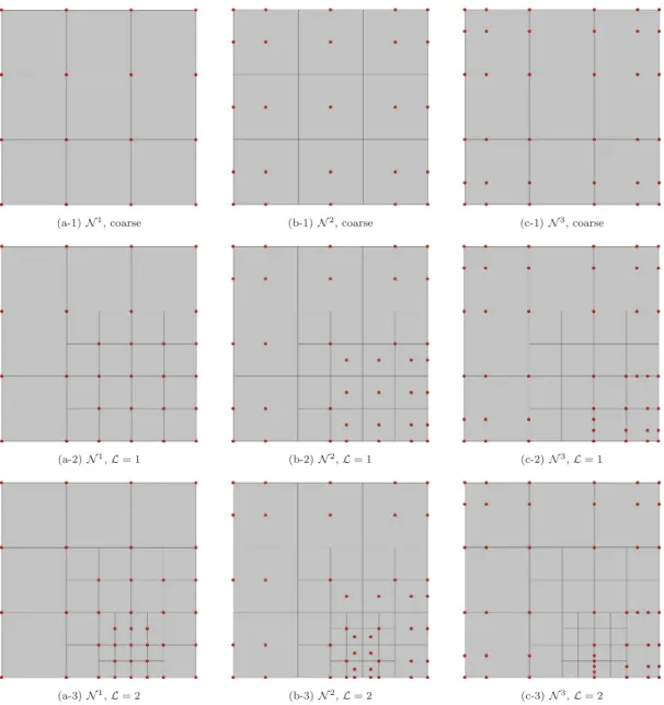
A numerical example for bulk discretization refinement at different orders is shown inFig. 3. The hierarchical discretizations of the surfaces are directly inherited from these bulk discretizations. Indeed, the refinements demonstrated inFig. 1correspond to the lower surfaces inFig. 3. The contact algorithms to be investigated next will be built on this observation. Note that only uI, not XI, is meaningful for a hierarchical basis function NI. Nevertheless, for graphical purposes, if NI is associated with a fine level basis function NℓJ then a control point has been placed at XℓJ inFig. 3. Consequently, some points are overlapping in the figure, for instance on the lower surface of N3for L = 2.
A hierarchical scheme may also be employed during the design process in order to endow an initially coarse geometry description with a number of fine features. In such a setting, one would first capture the base geometry exactly, excluding fine features such as a localized surface texture or a sharp protrusion. Subsequently, local hierarchical refinement would be employed to capture these features without altering the base geometry [40]. Once this is done, either an isoparametric formulation can be followed or further refinement may be carried out to improve the solution quality locally towards a subparametric formulation. In any case, in the context of isogeometric analysis, one starts from the premise that the reference geometry is exactly represented. As in standard finite element analysis, using an inexact geometry will lead to wrong stresses, and in particular to wrong contact tractions, unless refinement also updates the reference geometry.
3. Contact algorithm 3.1. Frictionless contact
The weak form of the linear momentum balance in a quasistatic setting without a body force for the frictionless contact of a slave body D(1)and a master body D(2)with spatial position vectors x(α)is symbolically denoted by
Fig. 3. Hierarchical refinement is demonstrated using Np( p = 1, 2 or 3) basis functions along each parametric direction, presently with unit weights (B-splines). The control points at each level are associated with the active basis functions.
where the bulk contribution is δGo= 2 α=1 R(α)o δF(α)·P(α)dV + Γo(α) δx(α)· p (α)dA (3.2)
and, introducing the notation ⟨•⟩ =Γc o
• dA, the contact contribution is
δGc = −⟨δg p⟩. (3.3)
In(3.2), F(α)and P(α)are the deformation gradient and the first Piola–Kirchhoff stress tensors, respectively, while R(α)o denotes the reference configuration and Γo(α) ⊂∂R(α)o denotes the portion of its boundary∂R(α)o with outward
unit normal N(α) where the Piola traction p(α) =P(α)N(α)is prescribed top(α). Within(3.3), Γc
o ⊂∂R(1)o indicates
the portion of the referential slave boundary that encompasses the potential contact zone inside which the referential contact pressure p and the normal gap g should ideally satisfy p> 0 and g = 0 while outside this zone p = 0 and
g < 0. For compactness, the notation for the contact contribution is specialized such that x will exclusively refer to a point on the spatial counterpart Γc of Γoc and y will indicate its closest-point projection on the master where the spatial outward unit normal isν. Hence, on Γoc, p(1)= pν in the absence of friction and
g = −(x − y) · ν. (3.4)
Denoting the referential counterparts of the position vectors x and y with X and Y, respectively, the displacement vectors
u = x − X, v = y − Y (3.5)
are introduced. The slave and master surfaces inherit their subparametric spatial surface discretizations, generally non-matching, directly from the hierarchical discretization of the volume. The coarse level shape functions of the slave/master volume will be denoted by N0K/M0L and the hierarchical ones by NI/MJ. Without distinguishing the surface basis functions with a separate notation, the referential position vectors referring to points on the surfaces are assigned the coarse level discretizations
X = n0X K =1 N0KX0K, Y = n0Y L=1 M0LY0L (3.6)
and the displacement vectors are assigned the hierarchical discretizations
u = nu I =1 NIuI, v = nv J =1 MJvJ. (3.7)
The summation limits will be omitted whenever the context makes these clear. Closest-point projection onto a hierarchically refined surface for the calculation of g does not pose a significant algorithmic difficulty and hence will not be discussed.
3.2. Contact discretization
An additional (kinematic) contact variable γ will be introduced and, together with the (kinetic) variable p, will be associated with the hierarchical discretization of the slave surface in the spirit of the mortar method. Specifically, the number of mortar basis functions BI is chosen to be nuand the span of each matches NI although the functions
themselves are not necessarily the same: γ = nu I =1 BIγI, p = nu I =1 BIpI. (3.8)
The variableγ is weakly linked to the physical gap via the condition ⟨BIγ ⟩ = ⟨BIg⟩which, upon defining the projected gap gI = ⟨BIg⟩and arranging the discrete values in vectors {γ } and {g}, leads to the formulation that recovers the kinematic contact variable from the normal gap:
{γ } = [Φ]–1{g} (full recovery). (3.9)
Here, the components of the overlap matrix [Φ] are ΦI J = ⟨BIBJ⟩. The numerical cost of solving this linear system of equations is small in comparison to the overall cost of the problem. Nevertheless, if row-sum lumping is applied to [Φ] to obtain a diagonal matrix then the solution of a linear system of equations is not necessary:
wI = ⟨BI
J
BJ⟩ −→ γI =gI/wI (lumped recovery). (3.10)
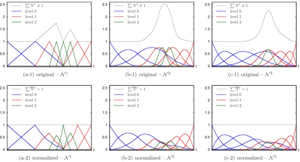
Moreover, if the mortar basis satisfies the partition of unity thenwI = ⟨BI⟩ such that one obtains the expression
γI = ⟨BIg⟩/⟨BI⟩that commonly appears in mortar-based contact algorithms. Both the full and the lumped recovery
Fig. 4. The hierarchical basis sets ofFig. 1are compared with their normalized counterparts. Note that the continuity of the normalized basis functions are now assessed with respect to the hierarchical element structure, represented by the knot structure in this one-dimensional case.
form are associated with the terms on the right-hand side of(3.9)and with the variationδgI, the latter appearing in
(3.3)which may be restated asδGc = −
Iδg
IpI. Additional mortar integrals which emanate from these terms
during linearization are standard [41].
In this work, two types of hierarchical mortar discretizations will be invoked. The first one inherits the hierarchical discretization of the slave surface displacement: BI = NI. However, this basis does not necessarily satisfy the partition of unity. A normalized basis
NI = N
I
J
NJ (3.11)
is introduced which does satisfy the partition of unity. The second choice is then BI = NI. The numerical cost of normalization is negligible. Moreover, normalization is straightforward to implement since it is only applied to the mortar basis. Note that the bulk discretization also does not satisfy the partition of unity but this does not pose any difficulties for the purposes of the present study and therefore no modification is needed. In the numerical investigations, the non-normalized set of mortar basis functions will be denoted by B and the normalized set by B. Normalization was discussed in [34], although it is possible to truncate the basis functions belonging to a refined level in order to ensure the partition of unity [35].
For the example ofFig. 1, the original and normalized basis functions are compared inFig. 4. Normalized basis functions share various properties of NURBS, but not all. For instance, if the NURBS basis functions are of order p and the coarse level knot vectors have no repeated interior knots then the normalized basis functions are p − 1 times continuously differentiable across the hierarchical element boundaries. Also, normalization distorts initially linear basis functions, similar to the transition from unit to non-unit weights with a standard N1discretization. However, unlike NURBS, a normalized basis function may attain multiple extrema across its span with the adopted hierarchical refinement algorithm (e.g. the last N3basis function from level 0 inFig. 4(c-2)).
Based on the hierarchical mortar discretization invoked above and a choice of BI, a relation betweenγI and pI
completes the contact formulation. This relation is specified through the constraint enforcement method. Below, an exterior point method is considered, followed by an interior point method. Combinations of choices for (i) the mortar basis, (ii) the recovery approach and (iii) the method of constraint enforcement deliver classes of contact algorithms, some of which have clear advantages or disadvantages and others which perform well only for special problems.
3.3. Exterior point method
The augmented Lagrangian method is a primal–dual exterior point method that covers the penalty and Lagrange multiplier methods as special cases and requires keeping track of an active set A. Presently, ifγI ≥0 is detected then the control point I becomes a member of A for which a Lagrange multiplierλI is activated such that the pressure in
(3.3)is formulated as
pI =λI+ϵγI (3.12)
whereϵ is a penalty parameter. λI will enforceγI to vanish for all I ∈ A and it should be deactivated whenever I leaves the active set, the latter detected if pI < 0 at any stage during the Newton–Raphson iterations. These conditions are incorporated through a Lagrange multiplier contribution to the weak form:
0 =δLc=
I
δλIω ×−γI if I ∈ A
ϵ–1λI if I ̸∈ A. (3.13)
Here, an additional scaling factorω is introduced, which can be simply chosen as unity. If, instead, one chooses ω as wIfrom(3.10), then the tangent matrix will be symmetric for the case of lumped recovery ofγI. The tangent matrix
will be unsymmetric in the case of full recovery. Note that although symmetry can be recovered by replacingωγI with gI for I ∈ A in this case, this would be inconsistent with(3.9)as well as with(3.12), whereγI is enforced to vanish rather than gI, and therefore can lead to an ill-defined problem with no solution. Using the Lagrange multiplier method, it is possible to directly enforce gIto zero, however this approach is intrinsically equivalent to lumping.
Overall, the full recovery approach closely resembles a recovery approach that was called unconstrained in [41,42], yet it is conceptually simpler and algorithmically more straightforward to implement. When all the control points on Γoc are active, full and unconstrained approaches will be equivalent. Hence, it is concluded that the full recovery approach also does not display locking and therefore passes the patch test on flat or curved interfaces, which is true for the lumped approach as well. On the other hand, while no advantages of unconstrained recovery over lumping were observed in earlier studies, numerical investigations to be presented will indicate that full recovery can display numerically superior properties in certain scenarios.
The value ofϵ has no influence on the solution quality for the augmented Lagrangian method and has only a mild influence with respect to convergence. The Lagrange multiplier method is obtained by omittingγI in(3.12), in which
case the value ofϵ in(3.13)becomes irrelevant. The penalty method is obtained as a primal exterior point method by omitting theλI term together with the Lagrange multiplier contributionδLc, in which caseϵ must be sufficiently large for an accurate solution without compromising convergence due to ill-conditioning. The linearization of these three possible formulations in order to determine the updates to the displacement and Lagrange multiplier degrees of freedom is largely standard and hence will not be discussed.
3.4. Interior point method
The interior point method to be employed in this work extends the presentation in [18] to the case of full recovery. Algorithmic details which are shared with this reference are omitted. In view of their considerable algorithmic similarity, this approach can easily be pursued starting from an augmented Lagrangian method implementation.
In interior point methods, the entirety of Γocis active at all times and the method is intrinsically built on the idea of maintaining a distance g < 0 between the surfaces. In the ideal case, based on the mortar discretization that has already been introduced, this can be readily achieved by explicitly enforcing a relation betweenγI and pI to hold at every Newton–Raphson iteration, similar to(3.12)for the exterior point method. Specifically, a classical barrier regularization pI = −µ/γI may be employed whereµ is a barrier parameter. However, this method would have two shortcomings. The first of these is its characteristic similarity to penalty regularization: an accurate solution requires a judicious choice ofµ, presently requiring a sufficiently small value without compromising convergence due to ill-conditioning. Interestingly, in sharp contrast with penalty regularization, this turns out to be a minor shortcoming such that µ can either be chosen as small as desired within a primal algorithm or it can be driven to zero automatically within a primal–dual version. The second shortcoming is major and algorithms for addressing it are central to modern interior point methods: surfaces may penetrate or touch each other during the Newton–Raphson iterations, leading to
In order to address the major shortcoming, an additional contact variable s is introduced such that at convergence it satisfies −γI =sI > 0 or, making use of(3.9), {s} = −[Φ]–1{g}. This statement is equivalent to the following gap
conditioncontribution to the weak form: 0 =δLc= I δpI gI+ J ΦI JsJ . (3.14)
The linearization of the weak form(3.1)of the linear momentum balance involves displacements as well as ∆ pIwhile the linearization of(3.14)entails the computation of
∆δLc= I δpI ∆gI+ J ΦI J∆sJ . (3.15)
In order to determine ∆sI, a primal algorithm can be pursued where µ is fixed at a predetermined value. At convergence, sI will satisfy pI =µ/sI. This local expression may be expressed as the complementarity condition
sIpI =µ, (3.16)
the linearization of which reads
sIpI+∆sIpI+sI∆ pI =µ (3.17)
and hence delivers an expression for ∆sI:
∆sI =(µ − sIpI −sI∆ pI)/pI. (3.18)
Substitution of this result into(3.15)completes the linearization of(3.14)and, together with the linearization of the linear momentum balance statement, leads to a system of equations that involves updates to the displacement and pressure degrees of freedom only, starting from an initial guess for the values of the displacements as well as for {sI, pI}. Note that updates to pIdetermine the updates to sI through(3.18). Since there is no active set in this interior point method, one must explicitly ensure that {sI, pI}remain positive after update. This is easily achieved by scaling the updates when necessary via fraction to the boundary rules, without altering the updates to the displacements.
One should note that it is tempting to enforce(3.16)strongly such that pI =µ/sI is directly employed at every iteration, eventually leading to an alternative primal algorithm which eliminates the pressure degrees of freedom. This version, however, turns out to have inferior convergence characteristics in comparison to the one summarized above. Moreover, the form presented here allows a relatively straightforward extension to the primal–dual algorithm in which µ is driven to zero automatically. In this context, it is noted that a difference between the lumped and full recovery approaches appears only in the gap condition(3.14). Although the statement of the complementarity condition in the form(3.16)also relies on a lumping argument, retaining this form is advantageous since it allows applying the primal–dual algorithm for the lumped setting without any modification—see [18] for details.
4. Numerical investigations 4.1. Remarks on setup
A series of numerical examples will be presented which concentrate on various features of different choices for the contact algorithm in the context of hierarchical discretizations. The effects or advantages of order elevation are not directly studied but orders ranging from two to six are employed in different examples to illustrate and benefit from this capability.
In all examples, an isotropic elastic material response is assumed. A Neo-Hookean material model will be employed in the case of finite deformations for which, in a d-dimensional setting, the strain energy function is
W =Λ1 2 (ln J)
2+Λ2
2 (J
where Λ1and Λ2are the bulk and shear moduli, respectively, and J = det [F] , C = FTF. The values of the moduli
are either prescribed directly or assigned indirectly through the values of the Young’s modulus E and the Poisson’s ratioν.
In the examples involving incremental loading, the simulation progress will be monitored by the variable t ∈ [0, T ]. When contact is initiated, the contact integrals are evaluated via Gaussian quadrature based on the (hierarchical) surface element structure of the slave (the upper body in all cases—indicated by the blue color in figures displaying the geometry). The advantages and shortcomings of such an approach for mortar-based methods have recently been assessed in [43] with respect to efficiency and accuracy. Presently, the order of integration employed ensures sufficiently accurate results. In general, for volume integrals, four integration points were employed along a parametric direction with up to N3discretizations and six points were employed for higher order discretizations up to N6. For contact integrals, the number was doubled with respect to these choices. The reader is referred to [21] and [10] for more accurate isogeometric mortar methods which employ segmentation-based integration schemes in the context of domain decomposition and contact, respectively. In the case of regularization, the absolute values of the penalty or barrier parameters will not be needed (except in Section4.4.1), hence their values are only reported when necessary relative to reference values µo = 10−5or ϵo, chosen to be ten times the maximum diagonal entry of the stiffness
matrix associated with the bulk contribution to the weak form. For the augmented Lagrangian method, the value of ϵ in(3.12)to be reported is set in the first Newton–Raphson iteration of a load step and subsequently kept constant within that load step.
4.2. Patch test
Basic features of different choices for the contact algorithm are first demonstrated with a flat interface patch test at large deformations. Only N2discretizations are employed, other choices displaying similar trends. Each body initially has a square geometry with dimension 1 and the initial gap between the bodies is 0.05. A displacement of 0.4 is then applied to the upper body. Presently, the bulk and shear moduli correspond to the choices of E = 1 andν = 0.3.
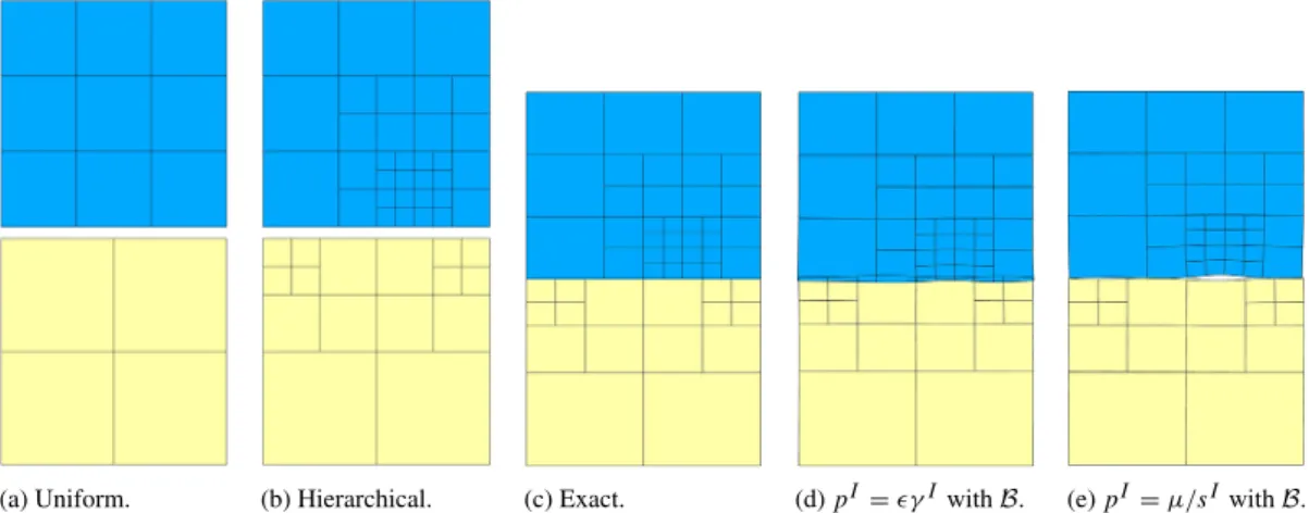
The geometry and results of the test are summarized inFigs. 5and6. With a uniform mesh, this patch test is passed for all combinations of different choices so that a constant pressure is obtained across the interface. With a hierarchical mesh, the test is passed for all combinations that enforce the constraints exactly, i.e. using the augmented Lagrangian method or with the primal–dual interior point method, which deliver a uniform pressure pexactthat results in a uniform
deformation. Neither the penalty method (with smallϵ) nor the primal interior point method (with large µ) passes the test if the original non-normalized mortar basis is used, leading to a non-uniform interface deformation with excessive penetration or gap. Retaining this basis, the patch test is satisfied with full recovery if the penalty method is employed but the primal interior point method still fails. Finally, with a normalized basis the test is satisfied irrespective of other choices for the contact algorithm. However, since the test is displacement controlled, a non-zero penetration due to a smallϵ leads to a slightly lower pressure compared to pexactfor the penalty method and a non-zero gap due to a large
µ leads to a slightly higher pressure for the primal interior point method.
The problem with the patch test arises only in the case of a exact enforcement of the constraints using the non-normalized mortar basis, and full recovery only helps in the case of the penalty method. The source of this observation is easily traced to the recovery statement(3.9):
• The normalized basis satisfies the partition of unity so that a constant g = c not only implies a constantγ = −s = c but also a constant γI = −sI = cirrespective of the method of recovery. Hence, pI = ϵc or pI = −µ/c is obtained that leads to p =ϵc or p = −µ/c.
• The original basis does not satisfy the partition of unity such that a constant g = c implies a constantγ = −s = c only with full recovery but even thenγI = −sI will not be a constant. Although pI will not be a constant in any case, a constant p will be implied if p is directly expressible in terms ofγ = −s. This is the case for the penalty method but not for the primal interior point method where, instead of the continuum expression p = µ/s, the approximate discrete expression pI =µ/sIis employed as remarked earlier in Section3.4.
In the limit of an exact enforcement of the contact constraints one obtains satisfactory results irrespective of the mortar basis or the recovery approach since enforcingγI =0 for all I is equivalent to enforcing g = 0 in all cases. Moreover, in Section4.3.3it will be demonstrated that in this limit retaining the approximate discrete expression pI = µ/sI does not adversely affect the results since the local solution quality is primarily controlled by the recovery approach.
(a) Uniform. (b) Hierarchical. (c) Exact. (d) pI =ϵγI with B. (e) pI =µ/sIwith B. Fig. 5. The patch test geometry of Section4.2is summarized. The hierarchical discretization of the upper body corresponds toFig. 3with N2. In (d) and (e), lumped recovery is employed.
Fig. 6. The analysis of Section4.2is summarized, based on the geometry inFig. 5. The exact result corresponds to an augmented Lagrangian or a primal–dual interior point method solution. Note that, here and in various upcoming examples, X1traces the referential position on the slave
surface in the horizontal direction—see(3.6).
4.3. Hertz contact problem
In order to illustrate some of the fundamental observations regarding the impact of different choices for the contact algorithm on the local solution quality, the classical Hertz contact problem is considered. The two-dimensional geometry of the contact setup with two bodies is borrowed from [41]. To summarize, the radius of curvature for each body is 1 and each one is displaced by 5 × 10⁻³ towards the other from an initial configuration where the surfaces touch at a point. For each body, E = 1 andν = 0.3.
In all figures, the distribution of the dimensionless pressure p/pmaxis monitored across the dimensionless position
r/rcontactwhere pmaxis the maximum pressure and rcontactis the half-width of the contact zone. The exact solution is
indicated with a gray line on the background. 4.3.1. Recovery comparison
Lumping of(3.9)is an algorithmically convenient simplification that has been successfully used in various earlier studies on isogeometric contact. To briefly demonstrate an advantage of full recovery, matching non-hierarchical discretizations are assigned to the slave and the master such that the radial directions are discretized with 72 N1 elements where as the angular direction is first discretized at a very coarse resolution with 96 N3 elements and subsequently this number is doubled/quadrupled to obtain coarse/medium resolutions.
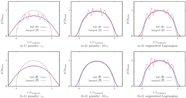
The results are summarized inFig. 7, by default based on the augmented Lagrangian method (employingϵ = ϵo
in(3.12)). At the very coarse discretization, the number of control points in the active set is very small. Nevertheless, full recovery is observed to already give a satisfactory answer that also rapidly approaches the exact solution with increasing resolution. Lumped recovery, on the other hand, delivers significantly oscillatory results at coarse resolutions yet these oscillations are not due to locking. Therefore a satisfactory solution is obtained beyond a
Fig. 7. The analysis of Section4.3.1is summarized. In the pressure plots, the points indicate the control point pressures. In the error plots, the error indicates the magnitude of the updates to the displacements scaled by the magnitude of the updated positions and the gray line indicates the convergence tolerance (10−9). The penalty parameter value corresponds to 10ϵoofFig. 9.
(a) Refinement (undeformed). (b) Contact zone (deformed).
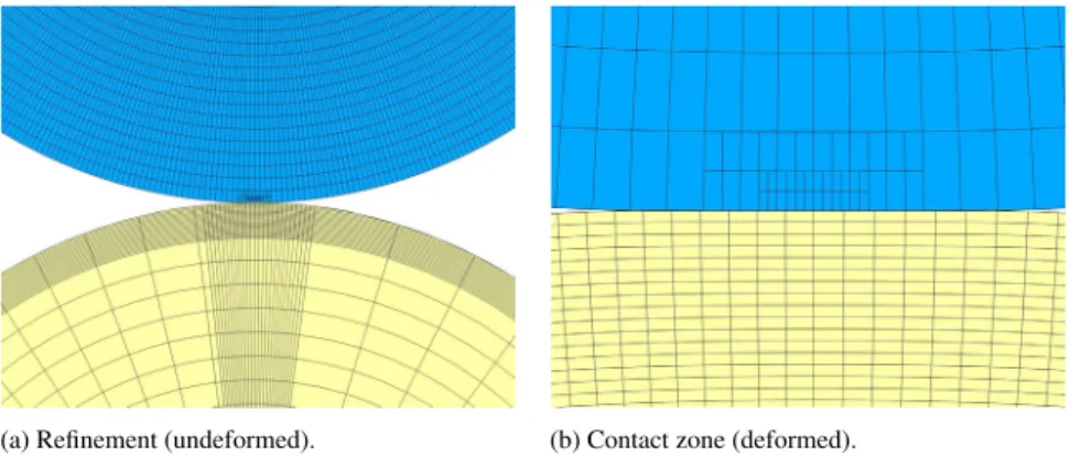
Fig. 8. The hierarchical refinement and the close-up of the contact zone are shown for the analysis of Section4.3.2.
sufficient number of control points in the active set. It is also observed that the number of iterations to achieve a prescribed convergence tolerance is smaller for full recovery, particularly at finer discretizations. Indeed, almost invariably for all the simulations carried out in this work full recovery required less iterations than lumped recovery, specifically when the constraints are enforced exactly. Consequently, one can state that the advantage of full recovery is higher efficiency with respect to a capability of delivering: (i) a better solution at coarse resolutions and (ii) a faster convergence at fine resolutions. Note that if, instead of augmented Lagrangian, the penalty method is employed with a reasonably large but not very large penalty parameter then the oscillations observed in lumped recovery are not displayed and an acceptable solution is obtained as also shown inFig. 7. However, this smoothing effect does not translate to an advantage of the penalty method but rather only highlights the importance of driving it to its limits to correctly assess its capabilities.
4.3.2. Exterior point method
Hierarchical discretizations will first be investigated with the exterior point method. To concentrate on the choice of the mortar basis functions, only the slave will be discretized hierarchically and with a rather coarse resolution to emphasize various aspects (Fig. 8). Initially, 36 N1elements are assigned to both the master and the slave in the radial
Fig. 9. The analysis of Section4.3.2is summarized, based on the discretization inFig. 8with exterior point methods for non-normalized (B) and normalized (B) mortar basis sets.
direction and 128 N2elements are assigned to the slave in the angular direction whereas 36 elements are assigned to the master. Subsequently, the mesh on the master is concentrated near the contact zone by knot relocation and the mesh on the slave is refined by two levels such that the refinement zone roughly corresponds to the contact zone, overall leading to non-matching meshes at the interface. The knot relocation on the master is slightly non-symmetric, which will induce slightly non-symmetric pressure distributions.
The results summarized inFig. 9 for the original mortar basis set is indicative of two aspects. First, unlike the uniform meshes inFig. 7, for lumped recovery with a non-normalized mortar basis even small values of the penalty parameter lead to oscillations that correlate with the structure of hierarchical refinement. Full recovery again displays a smoothness that is also retained at the exact constraint enforcement limit of augmented Lagrangian. At this limit, lumped recovery continues to display oscillations, but this time not due to hierarchical refinement but rather due to the coarseness of the hierarchically refined mesh, similar to the case ofFig. 7. This establishes a link to the second aspect, namely that the use of a normalized mortar basis removes the oscillations observed with the penalty method for lumped recovery. In the limit of augmented Lagrangian, however, lumped recovery again displays oscillations, which verifies that these are due to the coarseness of the mesh. Overall, for this example, one can state that the effect of normalization is only important for the penalty method with lumped recovery and normalization is not necessary at the augmented Lagrangian limit. At this limit, similar to uniform meshes, full recovery again delivers superior results since the hierarchical refinement is not sufficiently fine.
Additional analysis inFig. 10reinforces earlier statements. Here, the hierarchical mesh in Fig. 8is refined by uniformly subdividing each element by three along both parametric directions, thereby retaining the locations of the hierarchical transitions along the slave surface. The oscillations that were observed for the penalty method with a non-normalized mortar basis and lumping are now even further concentrated to spikes at the transition regions, thereby verifying that this combination does not benefit from refinement. In the augmented Lagrangian limit, however, the lumped recovery solution does benefit from refinement as predicted. As in earlier examples, full recovery displays a smooth result that only improves with refinement. In all cases, a difference between the normalized and non-normalized mortar basis is only apparent in the case of the penalty method with lumping and any difference is hardly noticeable for other combinations of choices even at a coarse resolution.
4.3.3. Interior point method
Fig. 11repeats the analysis ofFig. 9 based on the interior point method. The interior point method in a primal setting resembles the penalty method and in a primal–dual setting it enforces the contact constraints exactly so that the solution obtained is the same as the augmented Lagrangian solution. For this reason, almost all the observations
Fig. 10. Complementary analysis forFig. 9is presented using non-normalized (B) and normalized (B) mortar basis sets. Here, the coarse mesh corresponds to the resolution ofFig. 8and the fine mesh is obtained by subdividing each element by three along both parametric directions.
Fig. 11. The analysis ofFig. 9is repeated with interior point methods (µo=10−5).
stated earlier for the exterior point method apply, with one exception. For a non-normalized mortar basis, full recovery also leads to significant oscillations for the penalty method although the oscillations disappear in the primal–dual limit. This suggests that the observed issue is not a mesh resolution effect but rather due to the choice of the mortar basis functions as verified by the smooth results obtained with normalization. Overall, it can be stated that the variation in the solution quality for the Hertz problem with different combinations of choices for the contact algorithm correlates well with the preceding studies in Sections4.2and4.3.1. In the remaining sections, different choices for the contact algorithms will be tested in finite deformation contact problems with evolving contact interfaces.
4.4. Ironing problem
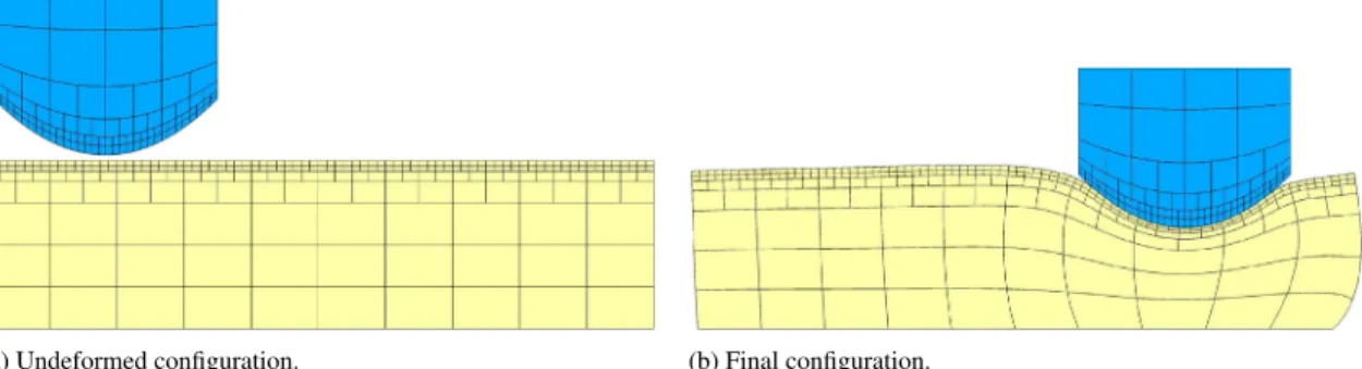
The ironing problem is considered as a benchmark case in two- and three-dimensional settings. The geometry of the problem is directly borrowed from [8], the changes being the downward displacement of the upper body (0.3) and its stiffness (103times larger than the lower one).
In this problem, the discretization of the bodies will be hierarchically refined towards the potential contact surfaces but the discretization on these surfaces will be uniform. This is achieved by refining all elements which lie adjacent to these surfaces, starting from the coarse level discretization that is visible in the corresponding figures displaying the geometry. The comparatively stiff slave body is assigned a N2discretization in all directions while the softer master is assigned a N6discretization in the direction of sliding in order to achieve a smoother evolution of the contact forces and a N2discretization in the remaining directions. Due to the uniform mesh on the potential contact surfaces, there is
(a) Undeformed configuration. (b) Final configuration.
Fig. 12. The two-dimensional ironing problem of Section4.4.1is summarized with three levels of hierarchical refinement (L = 3).
Fig. 13. The normal (FN) and tangential (FT) forces associated with the two-dimensional ironing problem ofFig. 12are summarized. Note that,
here and in upcoming examples, L indicates the number of hierarchical levels of refinement—see Section2.2.
no need to distinguish between normalized and non-normalized mortar basis sets in this problem. By default, an exact constraint enforcement will be pursued based on the augmented Lagrangian method (employingϵ = 0.1ϵoin(3.12)).
4.4.1. Two-dimensional case
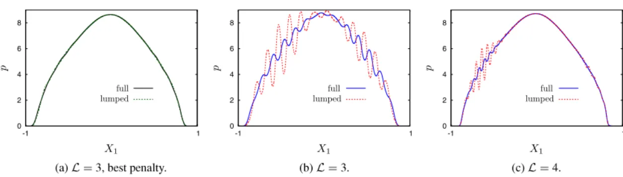
The two-dimensional test and the corresponding forces measured on the upper surface of the slave body are summarized inFigs. 12and13. Here, the fine mesh solution employs uniform refinement at the resolution of level 4 and delivers a converged force curve for which lumped and full recovery results are virtually overlapping, hence are not distinguished. The visible offset from the fine mesh solution for the normal force as well as the oscillation in the tangential force rapidly diminishes with hierarchical refinement. After four levels of hierarchical refinement, the forces still do not overlap with the fine mesh solution since refinement is highly localized near the contact surfaces and hence the solution is still significantly influenced by the coarse elements away from the contact zone. However, due to the fine meshes on the surfaces, the difference between full and lumped recovery diminishes with increasing refinement and after four levels of hierarchical refinement the two curves cannot be distinguished. Moreover, it is observed that full recovery displays smoother tangential contact forces at coarse resolutions, which correlates with earlier observations regarding smoother pressure distributions. On the other hand, it can also be observed that full recovery always overestimates the magnitude of the normal force in comparison to lumped recovery. This point will be revisited in Section4.5.
Fig. 14. The (non-Hertzian) pressure distributions for the analysis ofFig. 13are shown at t/T = 1. The best penalty solution is obtained with
ϵ = 104.
(a) Undeformed configuration. (b) Final configuration.
Fig. 15. The three-dimensional ironing problem of Section4.4.2is summarized with L = 1.
The forces inFig. 13are virtually overlapping for the augmented Lagrangian method and the primal interior point withµ = 10−5, hence are not distinguished. In comparison to global measures such as forces, local measures such as the pressure distribution are more sensitive to the choice of regularization parameters. The pressure distribution in the final configuration is compared inFig. 14for different contact algorithms. In these cases, a value ofµ = 10−8 also delivers virtually overlapping pressure distributions with augmented Lagrangian. Again, full recovery delivers a less oscillatory result than lumped recovery and, although the forces do not significantly improve beyond L = 3, the oscillations in the pressure significantly diminish with increasing hierarchical refinement. The best penalty regularization result with respect to the augmented Lagrangian limit for this example was obtained with ϵ = 104, which is similar in quality to the choice of µ = 10−4. At this value, there remains a difference with the force predictions of the augmented Lagrangian method (not shown) yet larger choices ofϵ prohibit convergence despite aggressive load step refinement. This is a major advantage of the primal interior method whereµ can be chosen to be even smaller than 10−8without compromising numerical performance—see also [18] for extensive discussions in the context of non-hierarchical discretizations. The smoothing effect in the pressure distribution that was earlier discussed in Section4.3is observable in this case as well at this insufficiently large value ofϵ.
4.4.2. Three-dimensional case
In order to demonstrate analysis capability, the ironing problem is revisited in a three-dimensional setting (Fig. 15). The results are summarized in Fig. 16. Here, the reference fine mesh solution employs: 16/3 elements in the horizontal/vertical directions of the slave, 60 elements in the sliding directions of the master and 9 elements in the remaining directions. The full recovery solution is chosen as the reference fine mesh solution in the coarse mesh and hierarchical solution figures.
Fig. 16. The normal (FN) and tangential (FT) forces associated with the three-dimensional ironing problem ofFig. 15are summarized.
On the finest uniform mesh that could be employed for this setup, full and lumped recovery solutions slightly differ from each other which suggests the need for further mesh refinement. Nevertheless, the full recovery solution is chosen as a sufficiently accurate reference solution. On the coarse mesh, both normal and tangential forces significantly differ from the reference solution. As in the two-dimensional case, full recovery overestimates the magnitude of the normal force at such coarse meshes. Only with a single level of refinement, the normal force predictions improve significantly, lumped recovery delivering a solution that is very close to the reference solution. For the tangential force, full recovery delivers a solution that again rapidly achieves smoothness in comparison to lumped recovery. Despite the superior performance of full recovery in most cases tested so far, the ironing problem suggests that this approach may be inferior to lumped recovery at considerably coarse meshes. This point is investigated next in detail.
4.5. Shell problem
In the following two- and three-dimensional test cases, thick-walled shell-like bodies are considered. The setup of this benchmark problem in three dimensions is borrowed from [41] and the two-dimensional case that is aimed to highlight potential shortcomings of full recovery is a direct simplification of this setup. The bodies are discretized with N2 elements in all directions for both cases. In order to concentrate on the comparison of the two recovery approaches, only the augmented Lagrangian method will be employed (with ϵ = 0.1ϵo in(3.12)). In agreement
with the discussions of Section4.3, the forces measured with lumped recovery in these test cases differ only slightly for normalized and non-normalized mortar basis sets due to the exact enforcement of the constraints. Moreover, the difference vanishes with increasing mesh resolution. Therefore, the choice of the mortar basis will not be distinguished in the presentation of lumped recovery results with the exception ofFig. 19.
4.5.1. Two-dimensional case
In the two-dimensional case (Fig. 17), the flat slave body is held stationary by fixing displacements at the left and right edges while the shell-like master body is displaced upwards towards the slave by displacement control in a similar fashion. Due to the symmetry of the setup, only the normal force FN exerted on the slave by the master
will be monitored. In the case of uniform meshes, the accuracy of the solution in this problem with respect to FN
is solely driven by the number of elements in the tangential direction. A mesh with a single element in the normal direction and 32 elements in the tangential direction already delivers a converged force profile that is identical for both full and lumped recovery. This solution is chosen as the reference. In subsequent discretizations, the master body is assigned the reference resolution while the slave is first coarsely discretized with 4 elements and subsequently elements adjacent to the potential contact surface is refined through one or two levels.
Fig. 17. The two-dimensional problem of Section4.5is summarized with L = 2.
Fig. 18. The normal force (FN) evolutions corresponding to the cases inFig. 17.
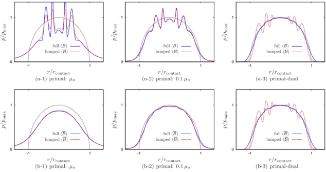
The results corresponding to the cases inFig. 17are summarized inFig. 18. In the lumped recovery case, a single level of refinement significantly improves the solution but the second localized refinement does not. This is expected since the mesh away from the contact zone is still significantly coarse. When full recovery is employed with the non-normalized mortar basis, a significantly different picture emerges where the solution quality deteriorates with increasing levels of refinement. By switching to a normalized basis, one obtains solutions that are comparable to the lumped recovery results.Fig. 17reflects this behavior, where deformation occurs with non-normalized full recovery as soon as the simulation starts despite the large distance between the bodies. Additionally, a gap is observed at the contact interface of the final configuration with normalized full recovery which reflects as an over-estimation of the force magnitude in comparison to the reference solution, similar to an earlier observation in Section4.4.1.
In order to investigate the source of the observations stated above, the evolution of the kinematic contact variable γ , which is the detection of the normal gap g by the mortar discretization, is depicted inFig. 19. Since lumping is a strong simplification of the recovery statement(3.9), the resultingγ profile is not a faithful reproduction of the actual gap g although the quality significantly improves with normalization. Nevertheless, irrespective of the mortar basis and the resolution, lumped recovery will not indicate contact before there is penetration (g< 0) at the potential contact interface sinceγIis proportional to the projected gap gI = ⟨BIg⟩and BIare non-negative. On the other hand, full recovery is intrinsically based on a faithful reproduction of g through the direct solution of(3.9). Hence, with or without normalization, it delivers aγ profile that conforms very accurately to g before contact is initiated. However, contact is initiated based on the values ofγI in all cases. Consequently, two shortcomings arise with full recovery. In
Fig. 19. For the cases inFig. 17, instances from the variation of the recovered normal gap (γ ) profiles are summarized for full (F) and lumped (L) recovery approaches with the non-normalized (B) and normalized (B) mortar basis sets. The actual normal gap (g) profile corresponds to theγ profile of the reference mesh solution.
Clearly, refinement at the coarsest level does not remove any basis functions in this example. By making use of Eqs.(3.6)–(3.8)may be expanded in this case explicitly as
γ = nu I =1 BIγI != n0x K =1 B0Kγ0K+ 2 ℓ=1 nℓu α=1 Bℓαγℓα (4.2)
where the first set is the coarse level contribution to the hierarchical discretization of γ and the remaining are associated with level 1 and 2 contributions such that n0x+
ℓnℓu=nu. The following observations may then be stated:
1. Non-normalized basis (BI = NI):The geometry is exactly represented by the coarse level basis functions N0K. If g could also be exactly represented by N0K, thenγℓα would vanish. This is indeed the case, for instance, if the
master body is also flat. When surfaces are curved, g depends on the discretization of both bodies and hence does not in general admit a representation based on N0K alone. This is the case for the present problem and some of the resulting non-zeroγℓα which essentially hierarchically refine the gap representation are in fact positive from the outset (Fig. 19(c-1)), thus leading to an immediate generation of a spurious force despite the distance between the bodies.
2. Normalized basis (BI =NI):The normalized forms N0Kcannot exactly represent the geometry. Indeed, even if the master body is also flat such that the gap is a constant at g = c, due to the partition of unity one necessarily obtains γI =cfor all I . Consequently, a spurious force is not generated. However, since NURBS discretizations are not
interpolatory,γI can lie far outside theγ profile, in particular at coarse discretizations (Fig. 19(d)). Therefore, contact can be initiated before penetration occurs, thereby leading to an over-estimation of the force magnitude due to displacement control, which was also observed in Section4.4.
The observation regarding the first shortcoming suggests that whenever refinement at a given level removes basis functions then this major shortcoming may be alleviated. This indeed has been verified in various test discretizations based on the present setup (not shown) and was also the case in the hierarchical discretizations employed in Sections4.3.2and4.3.3of the Hertz contact problem. However, the adopted hierarchical refinement algorithm does not guarantee removal in general and therefore such an analysis is not pursued further. One may speculate that a discretization of the pressure in a fashion similar to that of the surface through coarse (as in(3.6)) and hierarchical (as in(3.7)) contributions may resolve this issue. Another possibility would be to adopt an alternative hierarchical refinement algorithm that guarantees removal of basis functions from the refined zone (which would still require addressing the second shortcoming). The investigation of either possibility is a major task that shall not be undertaken in the present work.
The second shortcoming is in fact not special to hierarchical discretizations. For a non-hierarchical discretization, full recovery is similar in nature to checking contact with a node-to-surface (NTS) type formulation based on the projection of spatial control point positions onto the master surface. Despite this similarity, it is expected to perform significantly better than NTS due to the underlying mortar structure. Such a comparison is beyond the scope of this work. It is sufficient to note that either method would predict contact initiation more accurately with an increasing number of degrees of freedom on the potential contact surface since the control degrees of freedom would become increasingly interpolatory. It is highlighted that the size of the contact zone may be small—only the number of degrees of freedom will control the quality of contact detection. In the light of experience gained through the simulations carried out in this work, it can be stated that this shortcoming is minor: it is significant only at considerably coarse discretizations and rapidly diminishes with the refinement of the coarse level mesh or with a uniformly increasing refinement on the potential contact surface. This was indeed the case with the Hertz contact and ironing problems discussed earlier. Hence, one might even state that there is no shortcoming—at coarse resolutions lumping allows significant local penetration whereas full recovery leaves a gap. However, in the context of hierarchical discretizations, it is additionally important to investigate how much a contact algorithm benefits from local refinement. This last point is investigated next.
4.5.2. Three-dimensional case
In the three-dimensional setup with two thick-walled shells in sliding contact, the bodies are initially discretized coarsely with 6 elements along the tangential directions and a single element in the thickness direction. Subsequently, a hierarchical refinement concentrated in the contact zone is carried out through two levels to obtain the discretiza-tion depicted inFig. 21. The reference solution is based on a uniformly fine mesh at the level 2 resolution, namely 24 elements along the tangential directions and 4 elements in the thickness direction. This mesh delivers a sufficiently ac-curate but not converged results, hence each recovery method is explicitly compared with its corresponding fine mesh solution. The presented results are reliably obtained using the augmented Lagrangian method or the primal interior point with a sufficiently smallµ (10−5and beyond). In view of the fact that the use of a non-normalized basis re-quires significant care with full recovery (Section4.5.1), only normalized basis functions have been considered in this remaining example. Lumped recovery is only very slightly sensitive to normalization as in the two-dimensional case. The normal and tangential force evolutions are summarized inFig. 22. In the case of full recovery, detection of contact is based on the values of γI which are obtained through the solution of a linear system of equations that
(a) Level 0. (b) Level 1. (c) Level 2.
(d) Non-normalized hierarchical (B). (e) Normalized hierarchical (B).
Fig. 20. The refinement at each level, the active basis functions and the hierarchical mortar basis in non-normalized (B) and normalized forms (B) are depicted for the hierarchical N2discretization of the slave body inFig. 17.
Fig. 21. Simulation instances from the analysis of Section4.5.2with a hierarchical discretization that is localized in the contact zone.
contact surface. On the other hand, each degree of freedom detects contact independently in the case of lumped recovery. Consequently, it is structurally more amenable to benefiting from local hierarchical refinement. Indeed, the solution improves with both approaches after refinement yet lumped recovery delivers a solution that is remarkably close to the fine mesh solution while full recovery is still influenced by regions of coarse discretization far from the contact zone.
5. Conclusion
In this work, hierarchical local refinement has been applied to frictionless contact problems using mortar-based discretizations in the context of isogeometric analysis with NURBS. The developments were carried out along three branches of investigations. First, two different numerical representations of the actual normal gap across the contact interface were introduced, namely a full recovery approach that is based on the solution of a linear system of equations in addition to a lumped recovery approach as its simplification. Second, two choices of hierarchical mortar basis sets were considered, one based on the hierarchical surface discretization of the slave body which does not satisfy the
Fig. 22. The normal (FN) and tangential (FT) forces associated with the three-dimensional shell problem ofFig. 21are summarized. The
hierarchical solution locally refines the coarse mesh towards the fine mesh through two levels within the contact zone.
partition of unity and another based on the normalization of this set. Third, both exterior and interior point methods were applied for the enforcement of the contact constraints, including penalty and barrier type regularizations as inexact approaches as well as primal–dual algorithms which are exact. The investigations carried out within this third branch were complementary to both the first, in the sense that existing methods for lumped recovery were extended to the case of full recovery, as well as to the second, since the choice of the mortar basis set strongly influences the local and global solution quality. Overall, the results indicate the following:
• If hierarchical refinement is carried out towards uniform surface meshes then full recovery can display smoother force variations at the global level and more accurate pressure distributions at the local level.
• For local hierarchical refinement, full recovery should be accompanied by a normalized mortar basis but exact and inexact constraint enforcement methods are equally applicable. Lumped recovery, on the other hand, should preferably be accompanied by an exact enforcement method, but it may be employed with or without normalization. • On coarse meshes, full and lumped recovery approaches both have their advantages and disadvantages. However, lumped recovery is more amenable to benefiting from local hierarchical refinement within the potential surfaces of contact such that the forces improve more rapidly with increasing levels of refinement in comparison to full recovery.
The investigations which have been carried out are comprehensive yet by no means exhaustive. Among other possibilities, the consideration of different hierarchical refinement algorithms, possibly in an adaptive fashion, and the incorporation of friction within a thermomechanical setting stand out as two immediate paths for further research. Problems which share similarities in the algorithmic basis for the treatment of interfaces, such as domain decomposition and cohesive zones, may also benefit from such investigations. Finally, it would be of interest to consider numerically more efficient alternatives to mortar schemes, such as point-to-surface or collocation type algorithms, for problems where computation speed is of major concern. Numerical efficiency may be particularly important for the dynamic contact of complex three-dimensional bodies, for which it may also be advantageous to