Modeling a Supply Chain as a Queuing System
Peral Toktaş-Palut*. Füsun Ülengin**
*Systems Engineering Department, Yeditepe University, Đstanbul, Turkey, (e-mail: [email protected]).
**Industrial Engineering Department, Doğuş University, Đstanbul, Turkey, (e-mail: [email protected])
Abstract: This study investigates a two-stage supply chain consisting of multiple suppliers at the first stage and a manufacturer at the second stage. The suppliers and the manufacturer have limited production capacities. The system operates in a manufacture-to-order environment, i.e. the suppliers and the manufacturer employ make-to-stock and make-to-order strategies, respectively. The inventory of each component at each supplier is controlled via base stock policy. The aim of this study is to model the supply chain as a queuing system. Under the necessary assumptions, each supplier is modeled as an
/ / 1
M M make-to-stock queue. Moreover, the average outstanding backorders and the average inventory level of each supplier are derived using the queuing model. On the other hand, the manufacturer is modeled as a GI M/ / 1 queue after deriving an approximate distribution for the interarrival times of the manufacturer. Furthermore, the average number of jobs in the manufacturer’s system and the average outstanding backorders at the manufacturer are obtained using the queuing model.
1. INTRODUCTION
A company may operate in different manufacturing environments such as make-to-stock, make-to-order, or manufacture-to-order. In a make-to-stock system, the company reduces the time to fill customer orders by holding inventory. However, besides its competitive advantage, holding inventory also increases the costs and may give rise to other problems associated with keeping stock. If the company operates on a make-to-order basis, no inventory is held and a customer order triggers the manufacturing process. It is expected that in such a system, the delay in filling the customer orders is larger than that of a make-to-stock system. Finally, manufacture-to-order is a hybrid manufacturing strategy, in which the inventories for parts and semi-finished products are held; however, the final products are manufactured after receiving the customer orders. Compared with the other two systems, a manufacture-to-order system leads to lower holding costs than a make-to-stock system and shorter lead times than a make-to-order system.
This paper investigates a two-stage supply chain operating in a manufacture-to-order environment. The system consists of multiple suppliers and a manufacturer with limited production capacities. The suppliers operate on a make-to-stock basis and the manufacturer employs a make-to-order strategy. The manufacturer orders each component from a particular supplier and production cannot start until all components arrive. The inventory of each component at each supplier is controlled via base stock policy. Backorders are allowed in the system and the capacity of the backlog queue at each supplier is infinite. Finally, end-customer demand arrives in single units and it is stochastic.
In this study, the aim is to model the supply chain as a queuing system and to obtain the performance measures of interest, which are the average outstanding backorders and the average inventory level of the suppliers, the average number of jobs in the manufacturer’s system, and the average outstanding backorders at the manufacturer. To our knowledge, the queuing model of a two-stage capacitated supply chain with multiple members at the first stage has not yet been explored in the literature.
This paper is based on two basic assumptions: end-customer demands occur according to a Poisson process; and service times of the suppliers and the manufacturer are independent and exponentially distributed. Under these assumptions, each supplier can be modeled as an M M/ / 1 make-to-stock queue. On the other hand, to model the manufacturer as a queuing system, the interarrival time distribution of the manufacturer has to be derived first. Then, the manufacturer can be modeled as a GI M/ / 1 queue based on this distribution.
The paper is organized as follows. Section 2 presents a review of the related literature. In Section 3, an approximate distribution is developed for the interarrival times of the manufacturer. In Section 4, the supply chain is modeled as a queuing system using this approximate distribution and the aforementioned performance measures are obtained. Finally, concluding remarks are given in Section 5.
2. LITERATURE REVIEW
The first model of a series system with stochastic demand was presented in a study by Clark and Scarf (1960). They considered a multi-echelon inventory problem and defined
the optimal policy for finite planning horizons. The extension of their study to infinite horizons was performed by Federgruen and Zipkin (1984), and other refinements were made by Rosling (1989), and Chen and Zheng (1994). See Zipkin (2000) for a more detailed review of the related literature.
Besides the studies mentioned above, Lee and Zipkin (1992), Buzacott et al. (1992), and Gupta and Selvaraju (2006) studied the modeling of series systems with limited capacity. All of these studies considered a system in which each stage holds inventory managed by base stock policy. In addition, Buzacott et al. (1992) also considered an MRP system to initiate the work release to each stage. Since our paper aims at modeling a capacitated two-stage system, the modeling approaches of these studies are described in more detail below.
Under the assumptions of a Poisson demand process and exponential unit production times, Lee and Zipkin (1992) approximated the point process describing the release of units from a stage by a Poisson process and modeled each stage as an M M/ / 1 queue. The authors also defined some performance measures such as the average customer backorders outstanding, the average work-in-process inventory, and the average finished-goods inventory. By comparing the approximation estimates with the simulation results for two-stage and three-stage systems, they concluded that the approximation appears to be quite accurate.
Buzacott et al. (1992) developed bounds and approximations for shipment delays based on a sample path analysis. Assuming that demands occur according to a Poisson process and service times are exponentially distributed, the authors approximated the congestion at the second stage of a two-stage base stock system using an M M/ / 1 queue. They also derived the distribution of the time between releases to the second stage and developed an alternative approximation using a GI M/ / 1 queuing model. Comparison of the
/ / 1
M M and GI M/ / 1 approximations with the simulation results indicates that the GI M/ / 1 queuing model improves the accuracy of the predictions.
Finally, Gupta and Selvaraju (2006) proposed a modification to the approximations of Lee and Zipkin (1992) and Buzacott et al. (1992). They derived performance measures such as the average number of units that need to be processed at the second stage, the average inventory at each stage, and the average number of backorders outstanding for a two-stage system. They also investigated systems with more than two stages. The authors then defined a near-exact matrix-geometric procedure to compare their approximation with the others. Numerical tests showed that their approximation gives better results.
Before closing this section, it is worth mentioning the studies on single-stage make-to-stock queues, which date back to Morse (1958). One of the most fundamental studies in this area is by Buzacott and Shanthikumar (1993), who studied various make-to-stock queuing models and obtained their performance measures. Among the make-to-stock queues
they have investigated are M M/ / 1 and GI G/ / 1 queues for a system in which backlogging is permitted; and
/ / 1 / ,
M M Z M G/ / 1 / ,Z and GI G/ / 1 /Z queues for a system with lost sales. They also studied make-to-stock queuing models for systems with stopped arrival, and bulk demand.
Bai et al. (2004) derived the interdeparture time distributions for make-to-stock queues controlled via base stock policy. The main findings of their study are the interdeparture time probability distributions and squared coefficient of variations for the base stock inventory queues with birth and death processes, such as M M/ / 1, M M c/ / , and M M/ /∞ inventory queues.
Schwarz and Daduna (2006) investigated M M/ / 1 systems with inventory management. They computed the performance measures and derived the optimality conditions under different inventory management policies such as the
(
0, Q)
policy with and without an additional threshold for the queue length.
Finally, Jouini and Dallery (2008) considered ordinary and conditional first passage times in general birth and death processes. They highlighted that in case of Markovian interarrival and processing times, a make-to-stock system can be modeled as a birth and death process; and some performance measures can be obtained by computing the conditional first passage times. See Lee and Zipkin (1992) and Buzacott and Shanthikumar (1993) for a more detailed review of the literature in this area.
The distinguishing feature of our study is that there are multiple members at the first stage of the supply chain. Therefore, none of the results in the literature can be used to model the manufacturer as a queuing system in our study. The next section presents the derivation of the interarrival time distribution of the manufacturer, which is needed to approximate the congestion at the manufacturer using a queuing model.
3. INTERARRIVAL TIME DISTRIBUTION OF THE MANUFACTURER
The supply chain considered in this paper has two stages consisting of multiple suppliers and a manufacturer with limited production capacities. Let the number of suppliers be
n, where n≥2. The suppliers employ a make-to-stock strategy and manage their inventories via base stock policy. Let Si be the base stock level of supplier i for i= …1, , .n On the other hand, the manufacturer operates on a make-to-order basis, i.e. no inventory is held by the manufacturer.
It is assumed that end-customer demands occur according to a Poisson process with rate .λ The service times of supplier i are independent and identically distributed (i.i.d.) random variables having an exponential distribution with rate µi for
1, , .
i= … n The manufacturer has also i.i.d. and exponentially distributed service times with rate µM. Let ρi and ρM be
the traffic intensity of supplier i and the manufacturer, respectively, where traffic intensity is the ratio of the arrival rate to the service rate. For the stability of the system, it is assumed that 0<ρi < for all 1 i= …1, ,n and 0<ρM <1.
Under these assumptions, each supplier can be modeled as an / / 1
M M make-to-stock queue. On the other hand, the interarrival time distribution of the manufacturer has to be derived to model the manufacturer as a queuing system. For one supplier, Buzacott et al. (1992) have derived the probability density function f( ).
( )
t of the interdeparture times of the supplier, i.e. the interarrival times of the manufacturer given by( )
(
)
(
)
( )(
)
1 1 1 1 1 1 1 1 1 1 1 2 1 1 1 1 1 , S t S t A t S f t e e e µ λ λ µ λ ρ µ ρ λ µ ρ ρ + − − − − + − = − + − + − (1)where A denotes the interarrival time of the manufacturer. However, as the number of suppliers increases, deriving the distribution of the interarrival times of the manufacturer becomes mathematically intractable. This brings forth the need of an approximate distribution.
Recall that the manufacturer cannot start production until all components arrive. Hence, the supplier with the minimum base stock level is expected to affect the interarrival times of the manufacturer the most. Based on this expectation and according to (1), an appropriate approximation for the probability density function of the interarrival times of the manufacturer can be given by
( )
(
)
(
)
( )(
)
1 1 1 2 1 1 , j j j j j S t S t A j j j t S j j j f t e e e µ λ λ µ λ ρ µ ρ λ µ ρ ρ + − − − − + − − + − + − ≃ (2) where supplier j is the one with the minimum base stock level among all suppliers,1 i.e.1, , arg min i; i n j S = = … j ρ is the traffic intensity of supplier j; and µj is the service rate of supplier j.
From (2), the approximate expected value of the interarrival times of the manufacturer is calculated as
[ ]
1,E A
λ
≃ (3)
and the approximate variance is
( )
1 2 1 1 Var 1 2 . 1 j S j j j A ρ ρ ρ λ + − − + ≃ (4)Hence, the approximate squared coefficient of variation, which is the ratio of the variance to the square of the expected value, is given by
1
If more than one supplier has the minimum base stock level, then supplier j is the one with the highest traffic intensity among these suppliers.
1 2 1 1 2 . 1 j S j A j j C ρ ρ ρ + − − + ≃ (5)
To test the precision of the approximate interarrival time distribution of the manufacturer given in (2), simulation models are developed for two, three, and four suppliers. In each case, the end-customer demand rate is set to one. The traffic intensities of the suppliers and the manufacturer can take on three values: 0.50, 0.67, and 0.80. Three different values are also selected for the base stock levels of the suppliers: 3, 5, and 7. As considering all the combinations is too time consuming, Taguchi designs are created using Minitab 15, each with 27 runs.
The simulation models are developed using Arena 9.0. The replication length of each run is 10,000 time units and the number of replications is set to 10.
To test the precision of the approximate interarrival time distribution of the manufacturer, the Kolmogorov-Smirnov test is applied. The results indicate that at the 0.01 significance level, the approximate distribution fits the interarrival time data of the manufacturer in 79 of the 81 cases, producing an error of 2.47%. However, the exponential distribution fits the data in 23 of the 81 cases, giving an error of 71.60%. Note that the exponential distribution is also considered in this study since it has been used in the literature (Buzacott et. al., 1992; Lee and Zipkin, 1992; Gupta and Weerawat, 2006) to approximate the interarrival times of the second stage when there is one member at the first stage. Consequently, since the error for the approximate distribution is reasonable, it is concluded that the interarrival time distribution of the manufacturer can be approximated as given in (2). Using this approximate distribution, the manufacturer can now be modeled as a queuing system. The next section presents the queuing model and performance measures for the suppliers and the manufacturer, respectively.
4. THE QUEUING MODEL AND PERFORMANCE MEASURES
Recall that in our system, end-customer demands occur according to a Poisson process and service times of the suppliers are i.i.d. and exponentially distributed. Under these assumptions, each supplier can be modeled as an M M/ / 1 make-to-stock queue. Furthermore, the performance measures of interest are the average outstanding backorders and the average inventory level of each supplier.
Let I ti
( )
be the inventory level of supplier i at time t; and( )
i
B t be the outstanding backorders at supplier i at time t for 1, , .
i= … n Then, from Buzacott and Shanthikumar (1993), the average outstanding backorders at supplier i is calculated as
[ ]
1 , 1, , , 1 i S i i i E B ρ i n ρ + = = − … (6)[ ]
(
1)
, 1, , . 1 i S i i i i i E I S ρ ρ i n ρ − = − = − … (7)On the other hand, under the assumption that arrivals to the manufacturer form a renewal process, the manufacturer can be modeled as a GI M/ / 1 queue with the interarrival time distribution given in (2). Moreover, the performance measures of interest are the average number of jobs in the manufacturer’s system and the average outstanding backorders at the manufacturer.
For the mean number of jobs in a GI G/ / 1 queuing system, Shanthikumar and Buzacott (1980) investigated approximations that require only the squared coefficient of variations of the interarrival and service times, denoted by
2
A
C and 2 ,
S
C respectively. The authors recommended different approximations for the various values of C2A and
2
S
C as given below:
i. The approximation of Krämer and Langenbach-Belz (1976):
[
]
(
)
(
)
(
)
2 2 2 2 2 , , , 2 1 M A S M M A S M M C C E N ρ ρ g C C ρ ρ + + − ≃ (8)where NM denotes the number of jobs in the manufacturer’s
system and
(
)
(
)
(
)
(
)
(
)
(
)
2 2 2 2 2 2 2 2 2 2 2 2 1 1 exp , 1 3 , , 1 exp 1 , 1. 4 M A A M A S A S M A M A A S C C C C g C C C C C C ρ ρ ρ ρ − − − ≤ + = − − − ≥ + ii.The approximation of Marchal (1976):
[
]
(
)
(
)
2 2 2 2 2 2 2 1 . 2 1 1 M S A M S M M M M S C C C E N C ρ ρ ρ ρ ρ + + + + − ≃ (9)iii.The approximation of Page (1972) by adding a slight modification to the original formula:
[
]
(
)
(
)
(
)
(
)
2 2 2 2 2 1 . 2 1 2 1 1 exp 3 A S M M M M M S A M C C E N C C ρ ρ ρ ρ ρ + + − − − + − ≃ (10) In addition, there are two other approximations for the mean number of jobs in a GI G/ / 1 queuing system presented by Buzacott and Shanthikumar (1993). These approximations are given by[
]
(
)
(
)
(
)
2 2 2 2 2 1 2 2 1 2 M S M M A M S M M M M M S C C C E N C ρ ρ ρ ρ ρ ρ ρ ρ + − + + − + − ≃ (11) and[
]
(
)
(
)
(
)
2 2 2 2 2 1 . 2 1 2 M A S A A M M M M C C C C E N ρ ρ ρ ρ + − + + − ≃ (12)To select the best-fit approximation for the average number of jobs in the manufacturer’s system among the approximations given in (8)−(12), the simulation models described above are used. Then, the simulation results are compared with these approximations. Note that 2
S
C is equal to one since the service times of the manufacturer are exponentially distributed. Then, 2
A
C calculated from (5) and 2
1
S
C = are substituted into (8)−(12), and the average numbers of jobs in the manufacturer’s system are calculated accordingly.
The results indicate that in the case of two, three, and four suppliers, the approximation of Marchal (1976) given in (9) has the minimum average errors of 2.74%, 3.28%, and 4.09%, respectively. Since these errors are in acceptable ranges, we select the approximation of Marchal (1976), which leads to the average number of jobs in the manufacturer’s system given by
[
]
(
)(
)
(
)
(
)
(
)
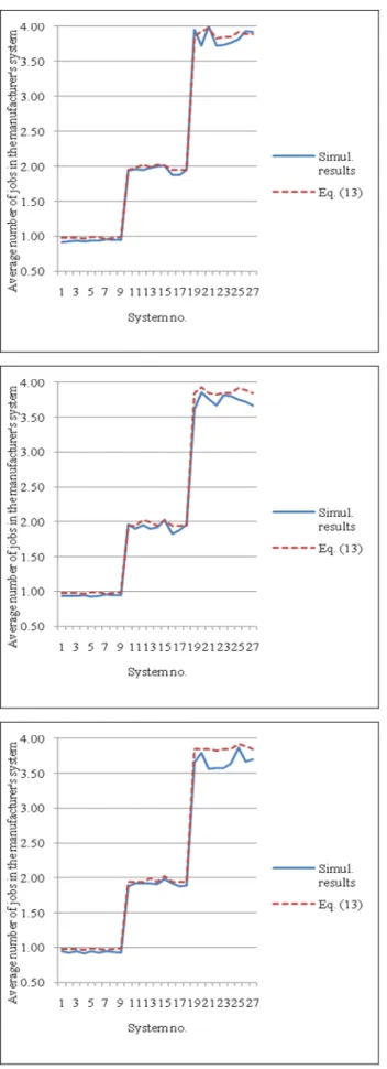
1 2 2 2 1 1 2 1 2 , 1 2 1 1 j S j M j j M M M M j M E N ρ ρ ρ ρ ρ ρ ρ ρ ρ + + + − − + + + − ≃ (13) where 1, , arg min i. i n j S = = …See Fig. 1 for the comparison of the simulation results with the approximation given in (13) for the case of two, three, and four suppliers.
The other performance measure of interest is the average outstanding backorders at the manufacturer, which is equal to the average number of jobs in the manufacturer’s queue since the manufacturer holds no inventory.
Recall that the approximate mean interarrival time of the manufacturer is calculated as 1λ in (3). In addition, since the service times of the manufacturer are exponentially distributed, the mean service time is given by 1µM. Then, using Little’s formula, it is easy to prove that
[
]
, M q M M E N = E N −ρ (14) where M qN denotes the number of jobs in the manufacturer’s queue.
Finally, substituting (13) into (14) yields that the average number of jobs in the manufacturer’s queue, i.e. the average outstanding backorders at the manufacturer, can be given by
[
]
(
)(
)
(
)
(
)
(
)
1 2 2 2 1 1 2 1 2 , 1 2 1 1 M j q M S j M j j M M j M E N E B ρ ρ ρ ρ ρ ρ ρ ρ + = + + − − + + − ≃ (15)where BM is the outstanding backorders at the manufacturer
and 1, , arg min i. i n j S = = …
(A)
(B)
(C)
Fig. 1. Comparison of the simulation results with the
approximation given in (13) for the case of (A) two suppliers; (B) three suppliers; (C) four suppliers
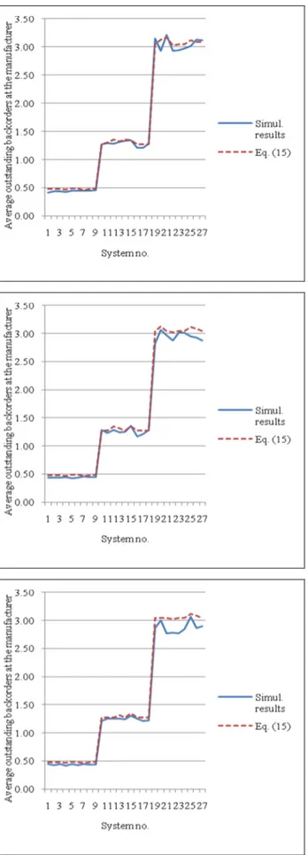
Fig. 2 depicts the comparison of the simulation results with the approximation given in (15) for the case of two, three, and four suppliers. For each system, the difference between the average number of jobs in the manufacturer’s system given in Fig. 1 and the average outstanding backorders at the manufacturer given in Fig. 2 is approximately equal to the traffic intensity of the manufacturer, as expected from (14). Consequently, this section presents the queuing model of the supply chain and derivation of the following performance measures: the average outstanding backorders and the average inventory level of the suppliers, the average number of jobs in the manufacturer’s system, and the average outstanding backorders at the manufacturer. The next section continues with concluding remarks.
5. CONCLUDING REMARKS
This paper examines a two-stage supply chain consisting of multiple suppliers and a manufacturer with limited production capacities. The suppliers operate on a make-to-stock basis and apply base make-to-stock policy to manage their inventories. On the other hand, the manufacturer employs a make-to-order strategy. The aim of this paper is to model the supply chain as a queuing system. To our knowledge, the queuing model of a two-stage capacitated system with multiple members at the first stage has not yet been explored in the literature.
Under the assumptions of a Poisson demand process and independent and exponentially distributed service times, each supplier is modeled as an M M/ / 1 make-to-stock queue. Furthermore, the average outstanding backorders and the average inventory level of each supplier are derived using the queuing model.
On the other hand, in order to model the manufacturer as a queuing system, an approximate distribution is developed for the interarrival times of the manufacturer. The idea behind the approximation is the expectation that the supplier with the minimum base stock level affects the interarrival times of the manufacturer the most.
To test the precision of the approximate interarrival time distribution of the manufacturer, simulation models are developed for the case of two, three, and four suppliers. The results show that the approximate distribution produces an error of 2.47%, meaning that it can be reasonably used as the interarrival time distribution of the manufacturer. Then, the manufacturer is modeled as a GI M/ / 1 queue. Moreover, the average number of jobs in the manufacturer’s system and the average outstanding backorders at the manufacturer are obtained using the queuing model.
As a further study, one could consider a system in which the manufacturer also operates on a make-to-stock basis. Then, the manufacturer could be modeled as a GI M/ / 1 make-to-stock queue and the new performance measures would be obtained accordingly.
(A)
(B)
(C)
Fig. 2. Comparison of the simulation results with the
approximation given in (15) for the case of (A) two suppliers; (B) three suppliers; (C) four suppliers
REFERENCES
Bai, L., B. Fralix, L. Liu, and W. Shang (2004). Inter-departure times in base-stock inventory-queues.
Queueing Systems, 47, 345−361.
Buzacott, J.A. and J.G. Shanthikumar (1993). Stochastic
Models of Manufacturing Systems. Prentice-Hall, New Jersey.
Buzacott, J.A., S.M. Price, and J.G. Shanthikumar (1992). Service level in multistage MRP and base stock controlled production systems. In: New Directions for
Operations Research in Manufacturing (G. Fandel, T. Gulledge, and A. Jones. (Ed)), 445−463. Springer, Berlin.
Chen, F. and Y. Zheng (1994). Lower bounds for multi-echelon stochastic inventory systems. Management
Science, 40, 1426−1443.
Clark, A. and H. Scarf (1960). Optimal policies for a multi-echelon inventory problem. Management Science, 6, 475−490.
Federgruen, A. and P. Zipkin (1984). Computational issues in an infinite-horizon, multiechelon inventory model.
Operations Research, 32, 818−836.
Gupta, D. and N. Selvaraju (2006). Performance evaluation and stock allocation in capacitated serial supply systems.
Manufacturing & Service Operations Management, 8, 169−191.
Gupta, D. and W. Weerawat (2006). Supplier-manufacturer coordination in capacitated two-stage supply chains.
European Journal of Operational Research, 175, 67−89. Jouini, O. and Y. Dallery (2008). Moments of first passage
times in general birth-death processes. Mathematical
Methods of Operations Research, 68, 49−76.
Krämer, W. and M. Langenbach-Belz (1976). Approximate formulae for the delay in the queueing system GI G/ / 1.
Congressbook, Eighth International Teletraffic Congress, 235.1−235.8.
Lee, Y.-J. and P. Zipkin (1992). Tandem queues with planned inventories. Operations Research, 40, 936−947.
Marchal, W.G. (1976). An approximate formula for waiting time in single server queues. AIIE Transactions, 8, 473−474.
Morse, P.M. (1958). Queues, Inventories and Maintenance:
The Analysis of Operational Systems with Variable Demand and Supply. John Wiley and Sons, New York. Page, E. (1972). Queueing Theory in OR, Operational
Research Series. Crane Russak, New York.
Rosling, K. (1989). Optimal inventory policies for assembly systems under random demands. Operations Research,
37, 565−579.
Schwarz, M. and H. Daduna (2006). Queueing systems with inventory management with random lead times and with backordering. Mathematical Methods of Operations
Research, 64, 383−414.
Shanthikumar, J.G. and J.A. Buzacott (1980). On the approximations to the single server queue. International
Journal of Production Research, 18, 761−773.
Zipkin, P.H. (2000). Foundations of Inventory Management. McGraw-Hill, Singapore.