Letter from the editors - [2009]

ACADEMY OF ACCOUNTING AND

FINANCIAL STUDIES JOURNAL

Mahmut Yardimcioglu, Karamanoglu Mehmetbey University

Accounting Editor

Denise Woodbury, Southern Utah University

Finance Editor

Academy Information

is published on the Allied Academies web page

www.alliedacademies.org

The Academy of Accounting and Financial Studies Journal is owned and published by the

DreamCatchers Group, LLC, and printed by Whitney Press, Inc. Editorial content is under the

control of the Allied Academies, Inc., a non-profit association of scholars, whose purpose is to

support and encourage research and the sharing and exchange of ideas and insights throughout the

world.

W

hitney Press, Inc.

Printed by Whitney Press, Inc.

PO Box 1064, Cullowhee, NC 28723

www.whitneypress.com

Neither the DreamCatchers Group or Allied Academies is responsible for the content

of the individual manuscripts. Any omissions or errors are the sole responsibility of

the authors. The Editorial Board is responsible for the selection of manuscripts for

publication from among those submitted for consideration. The Publishers accept

final manuscripts in digital form and make adjustments solely for the purposes of

pagination and organization.

The Academy of Accounting and Financial Studies Journal is owned and published

by the DreamCatchers Group, LLC, PO Box 2689, 145 Travis Road, Cullowhee, NC

28723. Those interested in subscribing to the Journal, advertising in the Journal,

submitting manuscripts to the Journal, or otherwise communicating with the Journal,

should contact the Executive Director at [email protected].

Academy of Accounting and Financial Studies Journal

Accounting Editorial Review Board Members

Atlanta Metropolitan College Atlanta, Georgia

Richard Fern

Eastern Kentucky University Richmond, Kentucky Manoj Anand

Indian Institute of Management Pigdamber, Rau, India

Peter Frischmann Idaho State University Pocatello, Idaho Ali Azad

United Arab Emirates University United Arab Emirates

Farrell Gean

Pepperdine University Malibu, California D'Arcy Becker

University of Wisconsin - Eau Claire Eau Claire, Wisconsin

Luis Gillman Aerospeed

Johannesburg, South Africa Jan Bell

California State University, Northridge Northridge, California

Richard B. Griffin

The University of Tennessee at Martin Martin, Tennessee

Linda Bressler

University of Houston-Downtown Houston, Texas

Marek Gruszczynski Warsaw School of Economics Warsaw, Poland

Jim Bush

Middle Tennessee State University Murfreesboro, Tennessee

Morsheda Hassan

Grambling State University Grambling, Louisiana Douglass Cagwin

Lander University

Greenwood, South Carolina

Richard T. Henage Utah Valley State College Orem, Utah

Richard A.L. Caldarola Troy State University Atlanta, Georgia

Rodger Holland

Georgia College & State University Milledgeville, Georgia

Eugene Calvasina

Southern University and A & M College Baton Rouge, Louisiana

Kathy Hsu

University of Louisiana at Lafayette Lafayette, Louisiana

Darla F. Chisholm

Sam Houston State University Huntsville, Texas

Shaio Yan Huang Feng Chia University China

Askar Choudhury Illinois State University Normal, Illinois

Robyn Hulsart

Ohio Dominican University Columbus, Ohio

Natalie Tatiana Churyk Northern Illinois University DeKalb, Illinois

Evelyn C. Hume Longwood University Farmville, Virginia Prakash Dheeriya

California State University-Dominguez Hills Dominguez Hills, California

Terrance Jalbert

University of Hawaii at Hilo Hilo, Hawaii

Rafik Z. Elias

California State University, Los Angeles Los Angeles, California

Marianne James

California State University, Los Angeles Los Angeles, California

Academy of Accounting and Financial Studies Journal

Accounting Editorial Review Board Members

University of Maryland-Eastern Shore Princess Anne, Maryland

Ida Robinson-Backmon University of Baltimore Baltimore, Maryland Ravi Kamath

Cleveland State University Cleveland, Ohio

P.N. Saksena

Indiana University South Bend South Bend, Indiana

Marla Kraut University of Idaho Moscow, Idaho

Martha Sale

Sam Houston State University Huntsville, Texas

Jayesh Kumar

Xavier Institute of Management Bhubaneswar, India

Milind Sathye University of Canberra Canberra, Australia Brian Lee

Indiana University Kokomo Kokomo, Indiana

Junaid M.Shaikh

Curtin University of Technology Malaysia

Harold Little

Western Kentucky University Bowling Green, Kentucky

Ron Stunda

Birmingham-Southern College Birmingham, Alabama C. Angela Letourneau

Winthrop University Rock Hill, South Carolina

Darshan Wadhwa

University of Houston-Downtown Houston, Texas

Treba Marsh

Stephen F. Austin State University Nacogdoches, Texas

Dan Ward

University of Louisiana at Lafayette Lafayette, Louisiana

Richard Mason

University of Nevada, Reno Reno, Nevada

Suzanne Pinac Ward

University of Louisiana at Lafayette Lafayette, Louisiana

Richard Mautz

North Carolina A&T State University Greensboro, North Carolina

Michael Watters

Henderson State University Arkadelphia, Arkansas Rasheed Mblakpo

Lagos State University Lagos, Nigeria

Clark M. Wheatley

Florida International University Miami, Florida

Nancy Meade

Seattle Pacific University Seattle, Washington

Barry H. Williams King’s College

Wilkes-Barre, Pennsylvania Thomas Pressly

Indiana University of Pennsylvania Indiana, Pennsylvania

Carl N. Wright Virginia State University Petersburg, Virginia Hema Rao

SUNY-Oswego Oswego, New York

Academy of Accounting and Financial Studies Journal

Finance Editorial Review Board Members

Florida A&M University Tallahassee, Florida

Ravi Kamath

Cleveland State University Cleveland, Ohio Roger J. Best

Central Missouri State University Warrensburg, Missouri

Jayesh Kumar

Indira Gandhi Institute of Development Research India

Donald J. Brown

Sam Houston State University Huntsville, Texas

William Laing Anderson College Anderson, South Carolina Richard A.L. Caldarola

Troy State University Atlanta, Georgia

Helen Lange Macquarie University North Ryde, Australia Darla F. Chisholm

Sam Houston State University Huntsville, Texas

Malek Lashgari University of Hartford West Hartford, Connetticut Askar Choudhury

Illinois State University Normal, Illinois

Patricia Lobingier George Mason University Fairfax, Virginia Prakash Dheeriya

California State University-Dominguez Hills Dominguez Hills, California

Ming-Ming Lai Multimedia University Malaysia Martine Duchatelet Barry University Miami, Florida Steve Moss

Georgia Southern University Statesboro, Georgia Stephen T. Evans

Southern Utah University Cedar City, Utah

Christopher Ngassam Virginia State University Petersburg, Virginia William Forbes

University of Glasgow Glasgow, Scotland

Bin Peng

Nanjing University of Science and Technology Nanjing, P.R.China

Robert Graber

University of Arkansas - Monticello Monticello, Arkansas

Hema Rao SUNY-Oswego Oswego, New York John D. Groesbeck

Southern Utah University Cedar City, Utah

Milind Sathye University of Canberra Canberra, Australia Marek Gruszczynski

Warsaw School of Economics Warsaw, Poland

Daniel L. Tompkins Niagara University Niagara, New York Mahmoud Haj

Grambling State University Grambling, Louisiana

Randall Valentine University of Montevallo Pelham, Alabama Mohammed Ashraful Haque

Texas A&M University-Texarkana Texarkana, Texas

Marsha Weber

Minnesota State University Moorhead Moorhead, Minnesota

Terrance Jalbert

University of Hawaii at Hilo Hilo, Hawaii

ACADEMY OF ACCOUNTING AND

FINANCIAL STUDIES JOURNAL

CONTENTS

Accounting Editorial Review Board Members . . . iii

Finance Editorial Review Board Members . . . v

LETTER FROM THE EDITORS . . . viii

UNOBSERVABLE PARAMETERS AND CONDITIONAL

ESTIMATES OF INTERNAL RATE OF RETURN . . . 1

Steven R. Fritsche, Howard University

Michael T. Dugan, The University of Alabama

EXECUTIVE COMPENSATION SCHEMES IN THE

BANKING INDUSTRY: A COMPARATIVE STUDY

BETWEEN A DEVELOPED COUNTRY AND

AN EMERGING ECONOMY . . . 19

Nelson Waweru, York University

Patrice Gélinas, York University

Enrico Uliana, University of Cape Town

GLOBALIZATION OF FINANCIAL MARKETS AND

REFLEXION TO TURKISH SMALL AND MEDIUM

SCALE ENTERPRISES: BASEL II . . . 35

Mahmut Yardimcioglu, Karamanoglu Mehmetbey University

Selcuk Kendirli, Hitit University

EARNINGS MANAGEMENT PRACTICES

FOR VENTURE IPO FIRMS . . . 47

Soon Suk Yoon, Chonnam National University (Korea)

INFLUENCE OF BUSINESS RISK ASSESSMENT

ON AUDITORS’ PLANNED AUDIT PROCEDURES . . . 69

Sandra Waller Shelton, DePaul University

Jo Lynne Koehn, University of Central Missouri

David Sinason, Northern Illinois University

IMPLEMENTATION OF ENTERPRISE RISK

MANAGEMENT (ERM) TOOLS – A CASE STUDY . . . 87

Ananth Rao, University of Dubai

SHOULD PROVISIONS OF THE SARBANES-OXLEY

ACT OF 2002 APPLY TO LOCAL GOVERNMENTS

IN ORDER TO IMPROVE ACCOUNTABILITY

AND TRANSPARENCY? . . . 105

Raymond J. Elson, Valdosta State University

Chuck Dinkins, City of Valdosta

AN OVERVIEW OF ACCOUNTING DEVELOPMENTS

IN ARCHAIC AND CLASSICAL GREECE . . . 123

William Violet, Minnesota State University Moorhead

LETTER FROM THE EDITORS

Welcome to the Academy of Accounting and Financial Studies Journal. The editorial

content of this journal is under the control of the Allied Academies, Inc., a non profit association of

scholars whose purpose is to encourage and support the advancement and exchange of knowledge,

understanding and teaching throughout the world. The mission of the AAFSJ is to publish

theoretical and empirical research which can advance the literatures of accountancy and finance.

As has been the case with the previous issues of the AAFSJ, the articles contained in this

volume have been double blind refereed. The acceptance rate for manuscripts in this issue, 25%,

conforms to our editorial policies.

The Editors work to foster a supportive, mentoring effort on the part of the referees which

will result in encouraging and supporting writers. They will continue to welcome different

viewpoints because in differences we find learning; in differences we develop understanding; in

differences we gain knowledge and in differences we develop the discipline into a more

comprehensive, less esoteric, and dynamic metier.

Information about the Allied Academies, the AAFSJ, and our other journals is published on

our web site. In addition, we keep the web site updated with the latest activities of the organization.

Please visit our site and know that we welcome hearing from you at any time.

Mahmut Yardimcioglu, Karamanoglu Mehmetbey University

Denise Woodbury, Southern Utah University

www.alliedacademies.org

UNOBSERVABLE PARAMETERS AND CONDITIONAL

ESTIMATES OF INTERNAL RATE OF RETURN

Steven R. Fritsche, Howard University

Michael T. Dugan, The University of Alabama

ABSTRACT

The conditional estimate of internal rate of return (CIRR) is intended to address several conceptual problems of the accounting rate of return (ARR). Nevertheless, researchers have raised concerns about the need to use an assumed project life and cash flow profile to calculate CIRR. The inability to directly measure IRR has prevented researchers from determining the impact of erroneous assumptions about firms’ project lives and cash flow profiles. The current study addresses this gap in the research literature by using simulation techniques to observe the IRRs, project lives, and true cash flow profiles for a sample of firms. By simulating the results of operations for a sample of firms, observations of the IRR, life of the composite project, and cash flow parameter were obtained to support a detailed evaluation of CIRR. The results of the current study indicate that assuming incorrect cash flow profiles affects the error with which CIRR estimates IRR. Moreover, the nature of the effect does not appear to be consistent with expectations. The results also indicate that assuming incorrect values for the life of the firm’s composite project will affect the estimation error in CIRR. The impact of erroneous assumed project lives appears to be more pronounced when CIRR is estimated for shorter sample periods. Growth did not significantly influence the estimation error in CIRR for the sample of simulated firms.

The results of the current study support prior research, which suggests that sensitivity analyses may not fully compensate for the use of assumed values for unobservable parameters. Additional research is needed to identify techniques that will allow decision makers to more accurately determine the parameters needed to calculate CIRR. Also, more information is needed about the unique characteristics of the firm and its economic environment that can increase the error with which CIRR estimates IRR.

INTRODUCTION

Even though evaluating the past investment decisions of commercial entities is critical to the success of investors, creditors, government agencies, and managers, identifying an appropriate measure upon which to base the evaluation remains difficult in several important contexts. The internal rate of return (IRR) generated by the firm’s portfolio of investments represents the theoretical ideal for some ex post performance evaluations, but this measure is unobservable in most cases. The firm’s stock return has limited usefulness as a substitute for IRR because it is not well suited to evaluating long-term profitability and asset returns (Schwert 1981). Moreover, those interested in evaluating privately held firms and sub-units of publicly held firms will not have access to stock returns. Often the only means by which investment performance may be assessed is through the use of profitability measures based on the firm’s external accounting reports.

Those who use accounting-based measures of profitability face a difficult choice. The most widely discussed and best understood profitability measure, the accounting rate of return (ARR), is relatively easy to calculate, but analytical research indicates that it exhibits sensitivity to accounting valuation bases and allocation methods, inflation, cash flow patterns, real growth rates, and length of asset lives in some models. (The literature investigating the relationship between ARR and IRR includes contributions by Harcourt (1965), Solomon (1966), Livingstone and Salamon (1970), Stauffer (1971), van Breda (1981), Fisher and McGowan (1983), and others. Jensen (1986) and Luckett (1984) provide reviews of this literature.) The conditional estimate of internal rate of return (CIRR), a profitability measure developed more recently by Salamon (1982 and 1985), addresses some of the ARR’s conceptual deficiencies by incorporating several of these factors. Building on the work of Ijiri (1978, 1979 and 1980), Salamon modeled the firm’s IRR as a function of inflation, investment growth rate, life of the firm’s composite project, the firm’s cash recovery rate (CRR), and the cash flow profile of the firm’s composite project. Nevertheless, researchers have expressed concern about the CIRR’s reliance on assumptions of a fixed real investment growth rate (Brief, 1985; and Stark 1989), an assumed constant cash flow profile (Brief, 1985; and Griner and Stark, 1991), assumed project lives (Brief, 1985; and Hubbard and Jensen, 1991), and a definition of cash from operations based on working capital (Lee and Stark, 1987; and Griner and Stark, 1988). In short, the CIRR possesses greater construct validity than ARR as an estimate of IRR, but several practical difficulties, especially the need to assume a project life and cash flow profile, have prevented it from being adopted as an unqualified successor to the

ARR.

The inherent limitations of research approaches used to date have prevented researchers from being able to determine whether erroneous assumptions about project lives and cash flow profiles result in significant measurement error in the observed value of CIRR. The extant analytical research has greatly increased our understanding of the relationships between CIRR and IRR, including the manner in which systematic and random error can affect CIRR. However, analytical models do not generally include sufficient information about the magnitudes of the variables involved to support inferences about the practical or statistical significance of identified sources of error. Empirical studies have investigated the relationships suggested by analytical research, but because IRR is not observable, the findings generally are based on an indirect empirical approach. Researchers using an indirect empirical approach have tried to draw inferences about the relationship between accounting-based profitability measures and IRR, based on the relationship between accounting-based profitability measures and variables believed to be related to IRR (e.g., Griner and Stark, 1991; and Fritsche and Dugan, 1996). Neither the analytical approach nor the indirect empirical approach has combined the ability to provide empirical evidence with a direct analysis of the relationship between accounting-based profitability measures and IRR.

The purpose of the current study is to address this gap in the extant literature by assessing the practical impact of using assumed values in the computation of CIRR. Computer simulation is used to construct an environment in which the actual IRRs, project lives, and cash flow profiles of a sample of simulated firms can be measured and compared to the conventional estimates or assumed values of these variables. This approach overcomes the inherent limitations of the previous research approaches described above. The use of simulation allows an analysis of the relationship between the error with which CIRR estimates IRR and the errors in the assumed values for the firm’s project life and cash flow profile. As such, it represents a worthwhile compromise between the analytical and indirect empirical approaches used in previous research.

The description of the current study is presented as follows. In the next section, the computer simulation is described in detail. Thereafter, the third section describes the variables used and the hypotheses tested. The fourth section sets out the research hypotheses. In the fifth section, the statistical tests and results are presented. The paper concludes with a summary.

SIMULATION METHODOLOGY

The data used in this study are based on the financial statement information of simulated firms. A Monte Carlo technique simulated the operations of a sample of firms for a total of 47 periods. During each of the periods, the simulated firms engaged in the activities typical of real firms. These activities included selling products, acquiring inventory, incurring operating expenses, arranging financing (by borrowing), and investing in long-term assets. The characteristics of the simulation are described below in sections devoted to exogenous economic factors, general financial and operating characteristics, and research design factors. Although every effort was made in the simulation process to capture the essential characteristics of real firms and the environments in which they operate, the results of the current study must be considered similar in some respects to those of laboratory experiments. Greater control over experimental variables and the improvements in measurement precision were obtained by limiting the ability to draw inferences about actual firms based on the results of the current study (Kerlinger, 1980; and Rivett, 1980). This scenario reflects the classic trade-off between internal validity and external validity inherent in such situations. Exogenous Economic Factors

Three features of the economic environment were determined exogenously because the processes needed to generate them are too complex to incorporate into the simulation program. First, the simulation program used United States Gross Domestic Product Implicit Price Deflators from 1949 through 1995 to represent inflation in the simulated environment. These inflation rates affected selling prices, input prices, operating costs, and the cost of plant asset purchases. Second, the complexity of simulating the market processes needed to derive changes in product demand resulted in the need to establish expected growth rates for product demand exogenously. Each firm was simulated using three different expected growth rates for quantity of products demanded: –5%, 0%, and +5%. These growth rates also affected operating costs and the real cost of plant asset purchases. Finally, the interest rates used to determine the cost of debt were the bank prime loan rates on short-term business loans as reported by the Federal Reserve Bank in St. Louis from 1949 through 1995.

General Financial and Operating Characteristics

As is the case for real firms, each simulated firm sold the lesser of two amounts of goods during each operating period: the quantity of goods demanded or the quantity of goods available for sale. As mentioned earlier, each firm was simulated under three different expected growth rates. In addition, the quantity of goods demanded in a given period was selected from a uniform distribution that ranged from ten percent above to ten percent below its expected value.

The quantity of inventory available in the current period was a function of the firm’s investment in plant assets and the true shape of the cash flow profile generated by that investment. Each firm was simulated using an increasing, level, and decreasing series of expected values for the output produced by each period’s investment in plant assets over the life of that investment. When the firm’s investments produced increasing expected values of output, the investment made in a given period produced output at 25 percent below the median expected value of output in the first year of the investment’s life. The expected value of the investment’s output increased by a uniform amount each period until, in the last year of the investment’s life, it produced output at 25 percent above the median expected value of output. The reverse of this pattern occurred in the case of a firm whose investments produced decreasing expected values of output. The resultant cash inflows from the sale of the firm’s output created increasing, level, and decreasing cash flow profiles for its investments.

Industry average data from Robert Morris Associates (1995) defined the initial financial position and operating characteristics of each firm. The initial composition of each firm’s balance sheet resulted from selecting an arbitrary value for total assets (1,000 currency units) and applying the percentages from the composite balance sheet data for the industry to this total. For manufacturing industries, the initial selling price per unit of output was 10 currency units, and applying 1 minus the composite gross margin percentage for the industry produced the initial cost per unit. Using median values of financial statement ratios for the industry, the simulation determined the following operating characteristics: (1) the percentage of inventory purchases paid within the year of purchase, (2) the percentage of sales revenues collected in the year of sale, (3) the percentage of operating and interest expenses paid within the year incurred, (4) the percentage of long-term debt maturing in the following period, (5) the percentage of total assets maintained in the form of cash, and (6) the average depreciable life of plant and equipment. Tables 1 and 2 describe the determination of operating characteristics in greater detail. Each firm’s accounts were updated to reflect each period’s transactions in accordance with basic double-entry accounting procedures.

The industry averages used to create the simulated firms were taken from the two-digit SIC classifications used by Salamon (1988). This approach produced a sample of 167 sets of industry averages for four-digit SIC classifications within the two-digit classifications. Using firms with Salamon’s industry groups should facilitate comparison of the results of this study with those reported by Salamon, thereby allowing a clearer interpretation of both sets of results.

Analytical research investigating the relationship between accounting-based profitability measures and IRR has consistently identified the firm’s depreciation method and inventory cost flow assumption as factors that may contribute to the observed differences between the two rates. Although ex ante there is less reason to expect accounting policy choices to affect CIRR than ARR, a choice concerning the inventory cost flow assumption and depreciation method had to be made for each firm in the sample. For this reason, each firm was simulated using both LIFO and FIFO inventory cost flow assumptions. To support extending the inferences drawn in the current study to those of previous research, each member industry of the two-digit SIC classes was randomly assigned to either the straight-line or sum-of-the-years’-digits groups, roughly in proportion to the observed usage patterns reported by Salamon (1988).

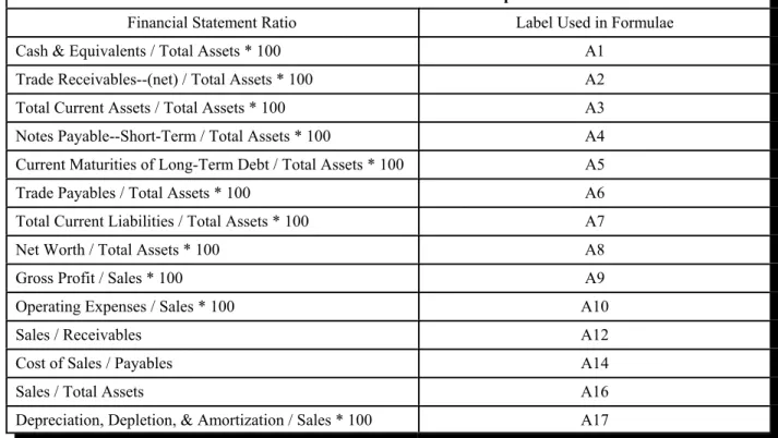
Table 1: Financial Statement Ratios Used in Computer Simulation

Financial Statement Ratio Label Used in Formulae Cash & Equivalents / Total Assets * 100 A1

Trade Receivables--(net) / Total Assets * 100 A2 Total Current Assets / Total Assets * 100 A3 Notes Payable--Short-Term / Total Assets * 100 A4 Current Maturities of Long-Term Debt / Total Assets * 100 A5 Trade Payables / Total Assets * 100 A6 Total Current Liabilities / Total Assets * 100 A7 Net Worth / Total Assets * 100 A8 Gross Profit / Sales * 100 A9 Operating Expenses / Sales * 100 A10 Sales / Receivables A12 Cost of Sales / Payables A14 Sales / Total Assets A16 Depreciation, Depletion, & Amortization / Sales * 100 A17

Table 2: Formulae Used to Calculate Simulation Parameters and Opening Balance Sheets for Simulated Firms

Value Calculated Formula

Cash Total Assets * A1 / 100

Trade Receivables Total Assets * A2 / 100

Inventory (Cost) (Total Assets * A3 / 100) - Cash - Trade Receivables Inventory (Units) Inventory (Cost) / (Selling Price * (1 - (A9 / 100)))

Gross Fixed Assets (Total Assets - Cash - Trade Receivables - Inventory (Cost)) * 2 Accumulated Depreciation Gross Fixed Assets / 2

Fixed Asset Purchases (Year 0) (A17 / 100) * (Total Assets * A16 / 100) Short-Term Notes Payable Total Assets * A4 / 100

Current Maturities of Long-Term Debt Total Assets * A5 / 100 Trade Payables Total Assets * A6 / 100

Accrued Liabilities (Total Assets * A7 / 100) - Short-Term Notes Payable - Current Maturities of Long-Term Debt - Trade Payables

Stockholders' Equity Total Assets * A8 / 100

Long-Term Debt Total Assets - Short-Term Notes Payable - Current Maturities of Long-Term Debt - Trade Payables - Accrued Liabilities - Stockholders' Equity

Table 2: Formulae Used to Calculate Simulation Parameters and Opening Balance Sheets for Simulated Firms

Value Calculated Formula

Operating Expenses (Year 0) (A10 / 100) * (Total Assets * A16 / 100) Unit Cost of Inventory (Year 0) Selling Price * (1 - (A9 / 100))

Expected Unit Demand (Year 0) Total Assets * A16 / Selling Price Portion of Purchases Paid for in Year of

Purchase

1 - (1 / A14) Portion of Sales Collected in Year of Sale 1 - (1 / A12) Portion of Operating Expenses Paid for in Year

of Incurrence

1 - (Accrued Liabilities / Operating Expenses (Year 0)) Portion of Long-Term Debt Maturing in Next

Period

Current Maturities of Long-Term Debt / Long-Term Debt Portion of Total Assets Maintained in the Form

of Cash

Cash / Total Assets

Finally, to assess the sensitivity of the results to the length of the estimation period used to calculate variables, three different estimation periods were used: 5, 10, and 15 periods. These estimation periods were based on the last 5, 10, and 15 periods of the 47 periods simulated for each firm. This approach left a “warm-up” phase of at least 32 operating periods. The “warm-“warm-up” phase allowed the simulated firm’s operating and financial results to stabilize before data accumulation began. As a result of the factors discussed above, the sample for each of the three estimation periods (5, 10, and 15 periods) contains a maximum of 3,006 observations. This number results from the following: 167 sets of industry averages x 2 inventory cost flow assumptions (FIFO and LIFO) x 3 expected growth rates (-.05, 0.0, and .05) x 3 actual cash flow profiles.

VARIABLE DEFINITIONS

A substantial amount of research has contributed to the development and testing of CIRR. This profitability measure is a complex elaboration of a capital budgeting tool developed by Ijiri (1978, 1979 and 1980). Ijiri suggested the use of a cash recovery rate (CRR) to measure investment performance. His cash recovery rate was based on the reciprocal of the traditional payback period. Ijiri demonstrated that under certain steady state conditions, the CRR was related to a return measure that converged to the firm’s IRR. Although Ijiri’s definition of CRR was based on working capital, Lee and Stark (1987) and Griner and Stark (1988) suggested that a cash flow definition is more consistent with the capital budgeting environment from which CRR developed. Thus, the current study defines CRR in the following way:

CRRit = NOCFit / GPAit, (1)

where NOCF is net operating cash flows before interest and taxes, and GPA is the average accounting value (cost) of plant assets during the period.

Salamon (1982) extended Ijiri’s work to develop a more complete representation of the relationship between CRR and an estimate of the firm’s real internal rate of return that Salamon described as cirr. The relationship derived by Salamon (1982) is as follows:

CRR = [(1 – pg)pn_gn _{/ 1 – p}n_gn_{] C [g}n _{– b}n _{/ g}n_{(g –b)] C[r}n_{(r – b) / r}n _{– b}n_{], (2)}

where r is 1 plus cirr, p is 1 plus the inflation rate, g is 1 plus the growth rate in investment (gross assets), n is the useful life of the firm's composite project, and b is an assumed cash flow parameter.

Several features of Salamon’s model require additional comment. First, because (2) explicitly incorporates price level changes, the resulting cirr is a conditional estimate of the firm’s real internal rate of return.

Second, growth rate in investment is defined as the logarithm of the ratio of the price level adjusted amount of gross plant assets at the end of the estimation period divided by the price level adjusted amount of gross plant assets at the beginning of the estimation period. This definition also was used by Salamon (1982, 1985 and 1988) and Griner and Stark (1988).

Third, the current study calculated the life of the firm's composite project, n, by first dividing gross property, plant, and equipment by depreciation expense for each year included in the estimation period. The average of those annual estimates was used as the value of n when the firm's depreciation expense was determined using the straight-line method. When the simulated firms used the sum-of-the-years'-digits depreciation method, n was calculated using the sum-of-the-years'-digits approach suggested by Buijink and Jegers (1989).

Finally, the calculation of cirr is conditioned on the assumed value of b, the cash flow parameter. If b is greater than 1, the cash flows of the firm’s composite project increase over its life, if b is less than 1, the cash flows of the firm’s composite project decrease over its life, and if b equals 1, the cash flows remain level. The current study calculated three different values of cirr, each based on one of three different values for b. Table 3 indicates the values used for b and the label assigned to the resulting values of cirr. (Salamon (1988) also included a definition of cirr that used a value of .8 for b when the firm used an accelerated depreciation method and a value of 1.0 when the firm used the straight-line depreciation method. Because growth and depreciation method combinations were exogenously determined, this formulation would not have a meaningful interpretation and is, therefore, not included.)

Table 3: Values Used for b to Compute Alternative Formulations of cirr

Values Used for b Label Used for cirr

.8 cirr1

1.0 cirr2

1.2 cirr3

As a basis for measuring the error with which cirr estimates irr, the current study employed a direct calculation of each firm’s real internal rate of return, irr, for the sample periods examined. To aid in the presentation of the research hypotheses later in the paper, the label used for this variable will be roi. The definition requires that the firm’s cumulative investment in assets, CUMINV, at the beginning and end of the

time interval be known and that the values of this variable be expressed in real magnitudes. The current study defines CUMINV as follows:

CUMINVit = CUMINVit-1 + [GPA+it / Atj=1 (1 + Dj)] – [GPA-it-n / At-nj=

1 (1 + Dj)] =CUMINVit-1 + gpa+it – gpa-it, (3)

where gpa- _{is the decrease in gross plant assets in the current period, discounted to time 0 dollars, and gpa}+ is the increase in gross plant assets in the current period, discounted to time 0 dollars. The simulation did not incorporate the market processes necessary to accommodate disposal of plant assets by sale. Therefore, the cost of plant assets and the related accumulated depreciation were removed from the firm’s accounts at the end of the assets’ lives. This approach to plant asset disposals is equivalent to the treatment given to assets that have been discarded. Values of CUMINV at the beginning and end of the sample periods in the study are used as beginning and ending economic values of the firm’s composite project. Put another way, the definition of real IRR, labeled roi, used in the current study relies on the assumed correspondence of the cumulative investment in the firm’s assets, discounted to time 0 dollars, to a market valuation, in real magnitudes, of those same assets. The formula used to calculate roi is as follows:

0 = CUMINVi0 – [En*t=1 [NOCFit – GPA+it / Atj=1(1 + Dj)] / (1 + roii)t] +

CUMINVin* / (1 + roii)t, (4)

In this formula, roi is calculated through an iterative process that terminates when a net present value of 0 is reached.

The formula used to calculate roi reflects the premise that most parties interested in evaluating the performance of a firm will be interested in a finite time interval, rather than the firm’s entire life. This premise is based on the impossibility of calculating profit rates for corporate entities with indefinite lives and the finite time horizons used by investors and other interested parties.

Having defined the necessary variables, the research questions addressed by the current study may be described. In the next section, these questions are expressed in the form of hypotheses that can be tested empirically.

HYPOTHESES

Before investigating the impact that imprecise estimates of unobservable parameters have on the error with which CIRR estimates IRR, it seemed appropriate to determine whether the total estimation error is significant. For this reason, the current study began by evaluating the significance of the percentage deviation of CIRR from IRR for the sample of simulated firms. Using percentage errors as the variable of interest avoids the impact of large values, while maintaining the possibility of a measure of central tendency with a value of zero. Let PE be defined as

where cirr and roi are as defined above in (2) and (6), respectively. If MPE is defined as the median value of PE, the first set of hypotheses can then be expressed as follows:

Ho1: MPE = 0 Ha1: MPE ¹ 0

By using median values of PE, the current study addresses this issue while avoiding questions about the normality of the variables’ distributions and also provides a more conservative (less powerful) test for the existence of a difference.

Next, the current study addressed the question of whether an incorrect assumption about the firm’s cash flow profile contributes significantly to the error with which CIRR estimates IRR. Several authors have expressed concern about the need to use assumed cash flow profiles when calculating CIRR (Brief, 1985; and Griner and Stark, 1991). Indeed, Salamon (1985 and 1988) acknowledged this limitation of CIRR, and, like other researchers, employed several assumed cash flow parameters to assess their impact on the outcomes of empirical research that relied on CIRR. Sensitivity analyses like those reported by Salamon and the results of Gordon and Hamer (1988) indicated that a strong association exists between alternative formulations of

CIRR. As a result, CIRRs based on different assumed cash flow parameters will generally yield the same

ranking of firms. However, Griner and Stark (1991) provided analytical evidence that use of an incorrect cash flow parameter will produce a CIRR containing error that is related to the firm’s investment growth rate. Moreover, the research reported by Stark, Thomas and Watson (1992) suggests that this systematic error will undermine the usefulness of CIRR in important practical applications. Thus, it appears on the basis of prior analytical research that a need exists for evidence of the magnitude of errors introduced by incorrect assumptions about the firm’s cash flow profile. Let M_jk represent the median PE contained in a simulated firm’s cirr when the firm’s composite project is producing an actual cash flow profile j and cirr’s calculation is based on an assumed cash flow profile k. If both j and k assume values indicating decreasing, level, or increasing cash flow profiles, then the second set of hypotheses may be expressed as follows:

H_o2: M₁₁ = M₁₂ = M₁₃ = M₂₁ = … = M₃₃

H_a2: At least one median is significantly different from the others.

This global test for significant differences in impact of assumed cash flow profiles given the actual profile indicates whether or not pairwise comparisons of the individual medians are warranted.

Finally, the computation of CIRR depends on two other variables that must be assumed or estimated from published data. Several authors have identified growth as a potential source of bias in CIRR. Additionally, both growth and the life of the firm’s composite project must be assumed or estimated from published data. As a means of assessing the incremental estimation error introduced by incorrect assumed cash flow profiles, the current study considered the following multivariate model:

PEit = $0 + $1TCFPit + $2git + $3PENit + ,it, (6)

where TCFP is a categorical variable indicating whether the firm’s true cash flow profile is decreasing, level, or increasing; g represents the firm’s expected growth rate (.05, 0.0, or -.05); and PEN _{is the percentage error}

with which n estimates the true life of the firm’s composite project. This model forms the basis for the third set of hypotheses:

Ho3: b1 = b2 = b3 = 0

Ha3: At least one coefficient is significantly different from 0.

Some researchers, including Griner and Stark (1991), have presented analytical models indicating that the estimation error in CIRR is a multiplicative function of firm’s cash flow profile and growth rate. Nevertheless, the current study uses the simple linear model in (8) because it allows a straightforward interpretation. Also, standard techniques exist to determine whether model misspecification is a significant concern.

The hypotheses described address concerns about the total error with which CIRR estimates IRR, the impact of using an incorrect cash flow profile when calculating CIRR, and the incremental contribution of incorrect cash flow profiles to the estimation error in CIRR. The next section describes the techniques used to test these hypotheses and the results of those tests.

RESULTS

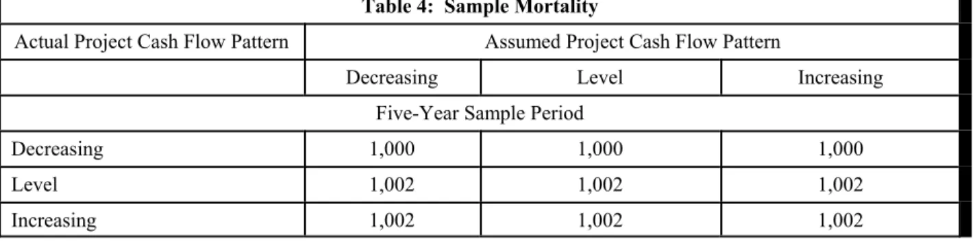
Before describing the results of the hypothesis tests, it may be helpful to point out an inherent problem associated with calculating cirr using (2) above. The calculated value of cirr is the result of an iterative process that involves substituting successive values for r in the equation and determining the closeness of the result to the observed value of CRR. When the result has converged on the observed value of CRR, defined as equality to six decimal places in the current study, the iterative process stops. In a limited number of cases, convergence could not be achieved. Table 4 indicates the sample sizes for the various combinations of assumed and actual cash flow profiles.

The first set of hypotheses concerned the percentage error with which CIRR estimates IRR. The Wilcoxon Signed Ranks Test (Gibbons, 1985) was used to determine whether or not the median percentage error was significantly different from zero. Table 5 summarizes the results of these tests. Regardless of the length of the sample period or the cash flow profile assumed, the null hypothesis was rejected at p £ .0001.

Table 4: Sample Mortality

Actual Project Cash Flow Pattern Assumed Project Cash Flow Pattern

Decreasing Level Increasing Five-Year Sample Period

Decreasing 1,000 1,000 1,000

Level 1,002 1,002 1,002

Table 4: Sample Mortality

Actual Project Cash Flow Pattern Assumed Project Cash Flow Pattern

Decreasing Level Increasing Ten-Year Sample Period

Decreasing 1,000 1,000 1,000

Level 1,002 1,002 1,002

Increasing 1,002 1,002 1,002 Fifteen-Year Sample Period

Decreasing 998 998 998

Level 998 998 998

Increasing 998 998 998

Note: In the absence of mortality, there would be 1,002 observations per cell.

Table 5: Wilcoxon Signed Ranks Test of Ho1: MPE = 0

Actual Project Cash Flow Profile Assumed Project Cash Flow Profile

Decreasing Level Increasing Five-Year Sample Period

Decreasing 180,199 134,397.5 138,657.5 (1,000) (1,000) (1,000) Level 150,320.5 100,761.5 110,775.5 (1,002) (1,002) (1,002) Increasing 10,236 -23,352.5 39,491.5 (1,002) (1,002) (1,002) Ten-Year Sample Period

Decreasing 143,388 131,328.5 140,983.5 (1,000) (1,000) (1,000) Level 138,291 123,758.5 136,202.5 (1,002) (1,002) (1,002) Increasing 112,911.5 109,686.5 131,762.5 (1,002) (1,002) (1,002)

Table 5: Wilcoxon Signed Ranks Test of Ho1: MPE = 0

Actual Project Cash Flow Profile Assumed Project Cash Flow Profile

Decreasing Level Increasing Fifteen-Year Sample Period

Decreasing 124,368.5 154,639.5 165.945.5 (998) (998) (998) Level 129,363.5 153,223.5 166,301.5 (998) (998) (998) Increasing 129,045.5 139,555 146,199.5 (998) (998) (998) Note: The first row reports the Wilcoxon S statistic, and the second row reports the number of observations. All

S statistics are significant at p # .0001.

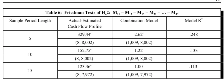
The impact of assuming an incorrect cash flow parameter when calculating CIRR is the issue addressed by the second set of hypotheses. Because each of the firms contributed an observation for each combination of assumed and actual cash flow profiles, the groups of observations are dependent. For this reason, the Friedman Test (Gibbons, 1985) was used to test the second null hypothesis. The Friedman Test is a nonparametric two-way analysis of variance. It accomplishes a test of medians for dependent samples by ranking the data within groups and treating the firm as the blocking factor. The results of the Friedman Tests are summarized in Table 6. The null hypothesis is rejected for all sample periods. In addition, the declining values of the F-statistic indicate that the impact of assuming an incorrect cash flow parameter decreases as the sample period lengthens.

Table 7 reports the results of pairwise Wilcoxon Signed Ranks Tests performed to further explore the results obtained from the Friedman Tests discussed above. All pairwise comparisons indicate a significant difference between the respective median percentage errors. Although it may seem reasonable to expect using an assumed cash flow profile that is consistent with the actual profile will generally produce a lower median percentage error, such a pattern is not evident in the results of the pairwise comparisons. For example, when the actual cash flow profile is level, one might expect that cirr₂, which is based on an assumption of a level cash flow profile, would estimate IRR with less error than either of the two alternative formulations. Similarly, it would be reasonable to expect cirr₁, which is based on the assumption of a decreasing cash profile, to contain less estimation error than the alternative formulations when the actual cash flow profile is decreasing. In fact, a consistent pattern emerges in which cirr₁ contains the highest measurement error and

cirr3 contains the lowest measurement error, regardless of the actual cash flow profile or length of sample period. Although the combination of actual and assumed cash flow profile influences the percentage error with which CIRR estimates IRR, the relationship between the combination and the amount of estimation error is not consistent with expectations.

Table 6: Friedman Tests of Ho2: M11 = M12 = M13 = M21 = … = M33

Sample Period Length Actual-Estimated Cash Flow Profile

Combination Model Model R2

5 329.44 c _2.62c _.248 (8, 8,002) (1,009, 8,002) 10 152.75 c _1.22c _.133 (8, 8,002) (1,009, 8,002) 15 123.46 c _{1.00 .113} (8, 7,972) (1,009, 7,972)

Note: The first row of each cell containing F statistic information is the F statistic, and the second row of the same cells reports the numerator and denominator degrees of freedom.

a _{p # .10} b _{p # .05} c _{p # .01}

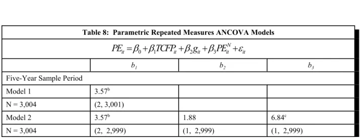
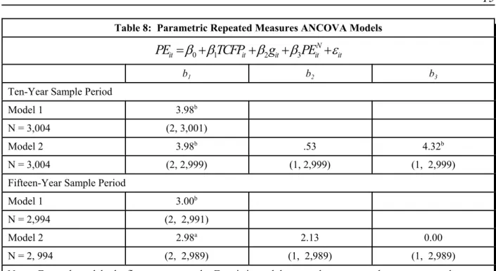
The third set of hypotheses concerned the impact of assuming an incorrect cash flow profile on the estimation error in CIRR while controlling for growth and the percentage error in estimated life of the firm’s composite project. Parametric repeated measures ANCOVA analyses were used to test the third null hypothesis for two reasons. First, the dependent variable for the model, cirr, included three observations for each of the simulated firms. By adopting a repeated measures approach, the dependency in these observations could be exploited to reduce experiment-wide error. (Wilkes Lambda tests of overall significance of the repeated factor (firm) indicated that the repeated factor was significant in all models for the ten- and fifteen-year sample periods. Such was not the case for the five-fifteen-year sample period.) Second, parametric ANCOVA techniques are more accessible than their non-parametric alternatives. Moreover, given the size of the sample, the distribution of the errors in the model was judged to be of limited grounds for concern. Table 8 presents the results of the ANCOVA analyses.

Several important inferences can be drawn from the repeated measures ANCOVA results reported in Table 8. First, the firm’s actual cash flow profile (TCFP) contributed significantly to the model’s ability to explain the error with which CIRR estimated IRR, regardless of the sample period used. Additionally, the significance of actual cash flow profile appeared to be unaffected by the inclusion of growth or project life estimation error. This evidence of model stability provides limited assurance that any interactions among the explanatory variables may be of little significance. Second, estimation error in the life of the firm’s composite project contributed significantly in the five- and ten-year sample periods. Finally, growth does not improve the ability to predict the estimation error in CIRR regardless of the length of the sample period. For the sample of simulated firms used in the current study, growth shows little relationship to the estimation error in CIRR.

Table 7: Wilcoxon Pairwise Comparisons of Percentage Errors

First Variable Compared Decreasing Actual Cash

Flow Profile

Level Actual Cash Flow Profile

Increasing Actual Cash Flow Profile Second

Variable Compared

cirr1 cirr2 cirr1 cirr2 cirr1 cirr2

Five-Year Sample Period cirr2 150,187 143,678.5 123,902.5 (1,000) (1,002) (1,002) cirr3 145,670 133,385 142,666.5 138,799.5 121,297.5 112,519.5 (1,000) (1,000) (1,002) (1,002) (1,002) (1,002)

Ten-Year Sample Period

cirr2 90,857 122,347.5 105,513.5 (1,000) (1,002) (1,002) cirr3 87,151 78,361.5 120,626.5 114,271 101,385.5 87,517 (1,000) (1,000) (1,002) (1,002) (1,002) (1,002)

Fifteen-Year Sample Period

cirr2 62,821.5 132,856.5 142,439.5 (998) (998) (998) cirr3 60,014.5 51.905.5 130.421.5 121,213.5 138,327.5 123,669 (998) (998) (998) (998) (998) (998) Note: The first row reports the Wilcoxon S statistic, and the second row reports the number of observations. All

S statistics are significant at p # .0001.

Table 8: Parametric Repeated Measures ANCOVA Models

it N it it it it

TCFP

g

PE

PE

=

β

+

β

+

β

+

β

+

ε

Five-Year Sample Period

Model 1 3.57b

N = 3,004 (2, 3,001)

Model 2 3.57b _{1.88 6.84}c

Table 8: Parametric Repeated Measures ANCOVA Models it N it it it it

TCFP

g

PE

PE

=

β

+

β

+

β

+

β

+

ε

Ten-Year Sample Period

Model 1 3.98b

N = 3,004 (2, 3,001)

Model 2 3.98b _{.53 4.32}b

N = 3,004 (2, 2,999) (1, 2,999) (1, 2,999) Fifteen-Year Sample Period

Model 1 3.00b

N = 2,994 (2, 2,991)

Model 2 2.98a _{2.13 0.00}

N = 2, 994 (2, 2,989) (1, 2,989) (1, 2,989) Notes: For each model, the first row reports the F statistic, and the second row reports the numerator and denominator degrees of freedom.

a _{p # .10} b _{p # .05} c _{p # .01}

CONCLUSION

The CIRR provides decision makers with a profitability measure that addresses many of the identified weaknesses of the ARR. It incorporates growth, inflation, the life of the firm’s composite project, and the shape of the firm’s cash flow profile. Although its calculation is more difficult, the CIRR’s greater construct validity may allow it to supplant the ARR in contexts where a profitability measure based on accounting information is required.

Unfortunately for users of accounting-based profitability measures, the CIRR also has been criticized. Extant analytical models indicate that CIRR may estimate IRR with error, including systematic error related to growth, because of its reliance on an assumed value for the firm’s cash flow profile. Moreover, CIRR relies on assumed values for another unobservable parameter, the life of the firm’s composite project. The inherent limitations of research approaches used to investigate the properties of CIRR have prevented researchers from assessing the magnitude of the estimation error introduced by incorrect assumptions about these two unobservable parameters.

The current study employed a simulation model to overcome the limitations of previous research. By simulating the results of operations for a sample of firms, observations of the IRR, life of the composite project, and cash flow parameter were obtained to support a detailed evaluation of CIRR. The results of the current study indicate that assuming incorrect cash flow profiles affects the error with which CIRR estimates

IRR. Moreover, the nature of the effect does not appear to be consistent with expectations. The results also

indicate that assuming incorrect values for the life of the firm’s composite project will affect the estimation error in CIRR. The impact of erroneous assumed project lives appears to be more pronounced when CIRR is estimated for shorter sample periods. Growth did not significantly influence the estimation error in CIRR for the sample of simulated firms.

The results of the current study support prior research, which suggests that sensitivity analyses may not fully compensate for the use of assumed values for unobservable parameters. Additional research is needed to identify techniques that will allow decision makers to more accurately determine the parameters needed to calculate CIRR. Also, more information is needed about the unique characteristics of the firm and its economic environment that can increase the error with which CIRR estimates IRR.

REFERENCES

Brief, R. P. (1985), ‘Limitations of Using the Cash Recovery Rate to Estimate the IRR: A Note’, Journal of Business

Finance & Accounting 12 (Autumn), 473-475.

Buijink, W. & M. Jegers (1989), ‘Accounting Rates of Return: Comment’, American Economic Review 79, 287-289. Fisher, F. M, & J. McGowan (1983), ‘On the Misuse of Accounting Rates of Return to Infer Monopoly Profits’,

American Economic Review 73 (March), 82-97.

Fritsche, S. R. & M. T. Dugan (1996), ‘Bias and Random Error in Accounting-Based Surrogates for Internal Rate of Return’, Journal of Applied Business Research 12 (Spring), 58-73.

Gibbons, J. D. (1985), Nonparametric Methods for Quantitative Analysis 2nd edition. (American Sciences Press). Gordon, L. & M. Hamer (1988), ‘Rates of Return and Cash Flow Profiles: An Extension’, Accounting Review 63

514-521.

Griner, E. H. & A. W. Stark (1988), ‘Cash Recovery Rates, Accounting Rates of Return and the Estimation of Economic Performance’, Journal of Accounting and Public Policy 7 (Winter), 293-311.

Griner, E. H. & A. W. Stark (1991), ‘On the Properties of Measurement Error in Cash-Recovery-Rate-Based Estimates of Economic Performance’, Journal of Accounting and Public Policy 10 (Fall), 207-223.

Harcourt, G. C. (1965), ‘The Accountant in a Golden Age’, Oxford Economic Papers 17 (March), 66-80.

Hubbard, C. M. & R. E. Jensen (1991), ‘Lack of Robustness and Systematic Bias in Cash Recovery Rate Methods of Deriving Internal (Economic) Rates of Return for Business Firms’, Journal of Accounting and Public Policy 10 (Fall), 225-242.

Ijiri, Y. (1979), ‘Convergence of Cash Recovery Rate’, in Y. Ijiri and A. B. Whinston (eds.), Quantitative Planning and

Control (Academic Press), 259-267.

Ijiri, Y. (1980), ‘Recovery Rate and Cash Flow Accounting’, Financial Executive 48 (March), 54-60.

Jensen, R. E. (1986), ‘The Befuddled Merchant of Venice: More on the “Misuse” of Accounting Rates of Return vis-a-vis Economic Rates of Return’, in M. Neimark, B. Merino, and T. Tinker (eds.), Advances in Public Interest

Accounting: 1 (JAI Press), 113-166.

Kerlinger, F. N. (1980), Foundations of Behavioral Research 3rd edition. (Holt, Rinehart, and Winston).

Lee, T. A. & A. W. Stark (1987), ‘Ijiri's Cash Flow Accounting and Capital Budgeting’, Accounting and Business

Research 17 (Spring), 125-132.

Livingstone, J. L. & G. L. Salamon (1970), ‘Relationship Between the Accounting and the Internal Rate of Return Measures: A Synthesis and an Analysis’, Journal of Accounting Research 8 (Autumn), 199-216.

Luckett, P. (1984), ‘ARR vs. IRR: A Review and Analysis’, Journal of Business Finance & Accounting 11, 213-231. Rivett, P. (1980), Model Building for Decision Analysis (John Wiley & Sons, Ltd).

Robert Morris Associates (1995), Key Business Ratios (Robert Morris Associates).

Salamon, G. (1982), ‘Cash Recovery Rates and Measures of Firm Profitability’, Accounting Review 57, 292-302. Salamon, G.(1985), ‘Accounting Rates of Return’, American Economic Review 75 (June), 495-504.

Salamon, G. (1988), ‘On the Validity of Accounting Rates of Return in Cross-Sectional Analysis: Theory, Evidence, and Implications’, Journal of Accounting and Public Policy 7 (Winter), 267-292.

Schwert, G. W. (1981), ‘Using Financial Data to Measure the Effects of Regulation’, Journal of Law and Economics 24 (April), 121-158.

Solomon, E. (1966), ‘Return on Investment: The Relation of Book-Yield to True Yield’, in R. K. Jaedicke, Y. Ijiri, and O. Nielsen (eds.), Research in Accounting Measurement (American Accounting Association), 232-244. Stark, A. W. (1989), ‘On Testing the Assumptions of the Cash Recovery Rate Approach to the Estimation of Economic

Performance’, Accounting and Business Research 19 (Summer), 227-285.

Stark, A. W., H. M. Thomas & I. D. Watson (1992), ‘On the Practical Importance of Systematic Error in Conditional IRRs’, Journal of Business Finance & Accounting 19 (April), 407-424.

Stauffer, T. R. (1971), The Measurement of Corporate Rates of Return: A Generalized Formulation’, Bell Journal of

Economics and Management Science 2 (Autumn), 434-469.

EXECUTIVE COMPENSATION SCHEMES IN THE

BANKING INDUSTRY: A COMPARATIVE STUDY

BETWEEN A DEVELOPED COUNTRY AND

AN EMERGING ECONOMY

Nelson Waweru, York University

Patrice Gélinas, York University

Enrico Uliana, University of Cape Town

ABSTRACT

This paper examined the level and structure of compensation schemes of directors (both executive and non executives) and other named officers in the banking industries of Canada and South Africa. We found a significant relationship between the CEO compensation and the market value of the firm. In addition the study examined the differences between the two countries, and the relationship between compensation schemes and the value of the firm. We found significant differences in the compensation structures and levels between the two countries.

INTRODUCTION

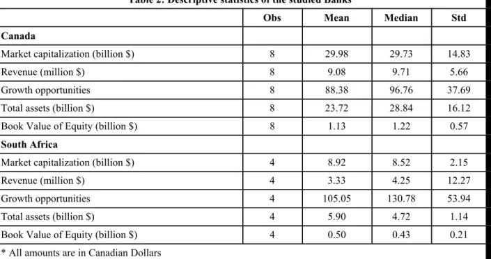
This paper examines the executive compensation schemes and practices of banks operating in Canada (a developed country) and South Africa (an emerging economy). In both countries a relatively small number of large banks dominate the national market, making the banking sector a unique research context and an interesting first step in the comparison of compensation paid in each country. Using a population of eight major publicly-traded banks in Canada and the four main banks in South Africa, we investigate the structure and level of executive compensation, defined as the sum of salary, annual bonus, the values of executive stock options and long term incentive plans (LTIPs). We discriminate between banks operating in Canada and those operating in South Africa and use contingency theory of management accounting to explain the differences. The term developing countries has been defined in a variety of ways by different authors mainly based on: 1) geographical location and 2) economic development. For example, Perera (1989) defines developing countries as those countries in the so-called Third World. Third World refers to those countries that do not belong to the Western world centered in the U.S.A, or the Eastern world with the former USSR as a centre. Wallace (1990) defines developing countries as those in the mid-stream of development and refers to an amorphous and heterogeneous group of countries mostly found in Africa, Asia, Latin America, the Middle East and the Oceanic.

South Africa is identified to represent developing countries since although classified so by the United Nations (2001) and the World Bank (2000), it lies on the upper income bracket of such countries. South Africa falls between both a developed and a third world country making it a good subject for examining the way in which compensation schemes are used in a developing country. South Africa is a developing country

to the extent that it is an exporter of raw materials rather than finished goods; the economy is heavily tied to one raw material, namely gold. South Africa has accelerated its privatization program with up to $24 billion of government assets to be released for divestiture (ADB, 2000).

The paper proceeds as follows; Section 2 describes the study theoretical framework. Section 3 describes the data and the methodology. Section 4 presents the results while section 5 discusses the results and presents a conclusion of the study.

THEORETICAL FRAMEWORK

Agency theory predicts that performance measures used for incentive purposes determine the direction of effort by the agent and that the incentive weight determines the amount of effort provided by the agent. The conventional theoretical framework for understanding reward contracts is in agency theory (Lambert 2001). Consequently the use of incentive contracts will lead to higher effort levels and increased performance on those dimensions that are being measured (Moers and Peek, 2000). The main prediction of the agency model is that pay should be sensitive to firm performance in order to induce managers to exert effort and thereby align the interests of the shareholders and managers (Jensen and Meckling 1976; Widener 2006).

Agency theory focuses on the risk characteristics of the enterprise (including any information asymmetry issues) as prime determinants of the shape and nature of reward contracts (Stathopoulos et al 2004). Emerging economy stocks are the most risky firms in our study (due to information asymmetry) and the developed economy stocks are the least risky, and so we expect to see differences between the reward contracts of South African Banks and those of the Canadian banks in our study. We expect South African bank executives to prefer a higher proportion of their compensation in long term incentives since more risk would lead to higher option values (Black and Scholes, 1973).

A similar argument could be made based on Smith and Watts (1992) who argue that a firm’s growth opportunities will have an impact on its executive compensation policy. They define growth opportunities as the ratio of book value of assets to firm value. We perceive a difference between growth opportunities in Canada and South Africa. Firms with higher growth opportunities are expected to offer more potential compensation to their managers. Firms with higher growth opportunities are also expected to offer more long term incentives than short term incentives (Bushman et al 1996). Higher possible levels of compensation are expected to motivate managers so that they can be able to exploit such future opportunities (Kato et al 2005). Conyon and Murphy (2000) argue that the generally higher compensation of US CEOs has put pressure on CEOs in the UK, Europe and elsewhere. Globalization of the market for executives has made it necessary for firms to benchmark their compensation against international companies. Further the growing influence of the shareholder value movement, has led to a greater focus on performance related compensation mechanisms, such as executive stock options. More recently, pressure on institutional investors such as unit trusts and insurance companies has increased the focus on financial performance and on executive packages (Stathopoulos et al 2004).

In some respects, Canada is to the US what South Africa is to the UK. For example, Canada is a smaller economy under the influence of the US and both countries share a history of close commercial ties. The same is true for South Africa and the UK. It is thus of interest to review prior research comparing US and UK. There are many similarities between the UK and the US in terms of their institutional framework and

the functioning of their capital and managerial labor markets. However, recent studies of compensation practices in the US and UK have yielded varying results. For example Ittner et al (2003) and Murphy (2003), report that equity-based pay is more prevalent among New Economy companies. Conyon and Murphy (2000) found substantial differences in pay practices, particularly in terms of a significantly greater use of stock options in the US than in the UK.

Contingency theory provides an explanation of why accounting systems vary between firms operating in different countries (Otley, 1980; Innes and Mitchell, 1990; Chapman, 1997; Waweru and Uliana 2005). According to Otley, (1980:413), “The contingency theory of management accounting is based on the premise that there is no universally appropriate accounting system applicable to all organizations in all circumstances. Rather contingency theory attempts to identify specific aspects of an accounting system that are associated with certain defined circumstances and to demonstrate an appropriate matching.”

According to Innes and Mitchell (1990) and Fisher (1995), the specific circumstances influencing management accounting comprise a set of contingent variables which may include but are not limited to: (1) the external environment, (2) the technology, (3) the organisation structure, (4) the age and (5) the firm’s competitive strategy and mission. These contingencies are regarded as important determinants of the design of the most appropriate management accounting system.

Demsetz and Lehn (1985) and Brickley and Dark (1987) find that the variation in ownership structure is explained in part by variation in firm characteristics such as size, location and ownership risk. Compensation practices are also heavily influenced by the regulatory framework within which the firm operates (Stathopoulos, 2004). We therefore expect the compensation practices of Canadian banks to differ from those of their counterparts in South Africa because many incentive plans rely on performance measures which emanate from the accounting systems, which are in turn contingent to country specific factors. Cultural differences between Canada and South Africa may also lead to different compensation arrangements. For example, the South African society is a high context culture with a strong sense of family while bargaining is not part of the South African business culture (Katja, 2001). In contrast Canada has a low context culture with low commitment to relationships (task more important than relationships) and very little is taken for granted during business bargaining (Hall, 1990).

Ang et al (2002) examined how US banks compensate their top management teams (i.e. the CEOs and the other top executive teams). They found that the CEOs receive not only greater pay in absolute dollars but are also rewarded more in relation to performance. However differences among the second tier executives were less clear and were generally statistically insignificant. In our study we investigated the compensation of the CEOs, other named executives and that of the non executive directors.

Chung and Pruit (1996) examined the factors that affect executive ownership, the market value of the firm and executive compensation. Their findings supported the notion that a firm’s market value, executive stock ownership and executive compensation are endogenous. Their findings are consistent with the view that the firm optimally establishes its managerial compensation plan in response to its operating environment.

Kato et al (2002) examined the adoption of stock options by Japanese firms. They reported that option plans are more likely to be adopted by firms with more growth opportunities.

To summarize, the following country specific factors are expected to create differences in the compensation schemes of the two countries:

a) Size: Canadian banks are larger in size than their South African counterparts. Canadian bank executives are therefore expected to receive higher compensation.

b) Technology: The level of technological development in Canada is higher than in South Africa. Information processing costs are therefore lower in Canada than in South Africa. Information processing costs will affect the nature of performance measures used in the determination of compensation schemes/levels.

c) Human resources: Like most developing countries, South Africa suffers from the problem of shortage of skilled human resources (Waweru, Hoque and Uliana, 2004). The shortage of skilled manpower in South Africa is expected to lead to higher demand for executives which would result to higher compensation levels.

d) Risk: Being an emerging economy, South Africa experiences higher information asymmetry than Canada. Higher risk would theoretically lead to higher option values (Black and Scholes, 1973). We therefore expect option values to be higher in South African than in Canada. South African executives are therefore expected to prefer long term pay to short term pay.

e) Regulatory/cultural differences. Executive compensation schemes

Compensation plans are vehicles of delivery of pay to the executives in a manner that attempts to motivate them to maximize shareholder’s wealth. The primary functions of an executive compensation plan are to attract, retain and motivate executives while controlling the potential agency costs associated with the separation of management and ownership. Anyangu (2005) identified the following as the main features of management compensation schemes.

a) The plan should be easy to monitor because it is based on objective criteria easily observed by all concerned parties and incapable of being manipulated.

b) The plan should prevent excessive perquisites to management and should minimize shirking thus encouraging expenditure decisions that benefit shareholders. c) The plan should have a long horizon to match the perspective of the shareholders. d) The plan should attempt to match managers’ risk to that of shareholders while recognizing that shareholders can diversify away from idiosyncratic risk of the firm more easily than managers who have their human capital tied to the firm’s future. e) Management compensation should be tied to changes in the shareholders’ wealth and if possible to management’s specific contribution to changes in shareholders’ wealth. For example a firm can under perform relative to its competition but still experience an increase in share price simply because the market went up.