Detecting structural change when the change point is unknown

7 ^ Р Т » ? ■

~'Л Ş» ч· ^ * ' f ': ’Ä '>. * t-í-.

IP «я Î? \ 7 «í^ * 5

-D ET E C T IN G STR U C TU R A L C H A N G E W H E N THE CH ANGE POINT IS U N K N O W N

A THESIS PRESENTED B Y SIDIKA BAŞÇI

TO

THE INSTITUTE OF

ECONOMICS AND SOCIAL SCIENCES

IN PARTIAL FULFILLMENT OF THE

REQUIREMENTS

FOR THE DEGREE OF M ASTER OF

ECONOMICS

BILKENT UNIVERSITY

Ч Рк

3 ^ 3 5

t 3 S 5

I certify that I have read this thesis and in my opinion it is fully adequate, in scope and

in quality, as a thesis for the degree of Master o f Economics.

I certify that I have read this thesis and in my opinion it is fully adequate, in scope and

I certify that I have read this thesis and in my opinion it is fully adequate, in scope and

in quality, as a thesis for the degree o f Master o f Economics.

L h o k k & y j t e

Assist.Prof,Dr.ChiranjitM ukhopadhyay

Approved by the Institute o f Economics and Social Sciences

A B S T R A C T

DETECTING STRUCTURAL CHANGE WHEN THE CHANGE POINT IS

UNKNOWN

SIDIKA BAŞÇI

M ASTER OF ECONOMICS

Supervisor: Prof. Dr. Asad Zaman

May 1994

There are various tests which are used to detect structural change when the change point

is unknown. Among these widely used ones are Cumulated Sums (CUSUM) and CUSUM

o f Squares tests o f Brown, Durbin and Evans (1975), Fluctuation test o f Sen (1980) and

Ploberger, Krämer and Kontrus (1989). More recently, Andrews (1990) suggests Sup F

test and shows that it performs better than the above stated tests in terms o f power. The

problem with these tests is that they all assume stable variance although the regression

coefficients change while moving from one regime to the other. In this thesis, we relax this

assumption and suggest an alternative test which also allows heteroskedasticity. For this

aim, we follow the Bayesian approach. We also present some of the Monte Carlo study

results where we find that Bayesian test has superiority over the above stated tests in

terms o f power.

Key Words: Structural Change, Unknown Change Point, Heteroskedasticity, Bayesian

Ö Z E T

DEĞİŞİM NOKTASININ BİLİNMEDİĞİ DURUMDA YAPISAL DEĞİŞİMİN

SINANMASI

SIDIKA BAŞÇI

Yüksek Lisans Tezi, İktisat Bölümü

Tez Yöneticisi: Prof. Dr. Asad Zaman

Mayıs 1994

Değişim noktasının bilinmediği durumda yapısal değişimin sınanması amacıyla kul­

lanılan pek çok farklı test vardır. Bunların arasında en çok kullanılanları Brown, Durbin

ve Evans (1975) tarafından önerilen Birikmiş Toplamlar (CUSUM) ve Birikmiş Toplamlar

Karesi, Sen (1980) ve Ploberger, Krämer and Kontrus (1989) tarafından önerilen Dal­

galanma testleridir. Daha yakın zamanda Andrews (1990) Sup F testini önermiştir ve

bu testin yukarıda belirtilen testlerden daha güçlü bir test olduğunu göstermiştir. Bütün

bu testlerde var olan problem hepsinin bir kısımdan diğer kışıma geçerken regresyon kat­

sayılarının değiştiğini varsaymasına rağmen varyansı sabit tutmalarıdır. Bu tezde, bu

varsayım hafifletiliyor ve varyans değişimini de göz önüne alan alternatif bir test öneriliyor.

Bu amaca Bayesyen yaklaşımla ulaşılıyor.Tez içerisinde, Bayesyen yaklaşımla elde edilen

testin daha güçlü olduğunu gösteren Monte Carlo çahşması sonuçları da yer almaktadır.

Anahtar Kelimeler: Yapısal Değişim, Bilinmeyen Değişim Noktası, Varyans Değişimi,

Acknowledgements

I would like to express my gratitude to Prof. Dr. Asad Zaman for his valuable supervision

and for providing me with the necessary background. Special thanks go to Assist. Prof.

Chiranjit Mukhopadhyay for his helps in camputations of the Bayesian tests. I also would

like to thank Assoc. Prof. Osman Zaim for his valuable comments. I appreciate the help

o f my sister in law, Özlem Başçı for letting me to use her computer for the simulations

which takes quite a considerable time.

I am thankful to my husband Erdem who gave strength to me at the times that I feel

Contents

3 Assessment of Loss From not Knowing the Change Point 7 3.1 Chow T e s t ... 7 3.2 Sup F Test ... 9 3.3 Assessment of L o s s ... 11 4 An Alternative Approach 13 4.1 Bayes’ T h eorem ... 13 4.2 The Model ... 14 4.3 Priors o f the M o d e l... 16

4.4 The Posterior A n a ly sis... 17

4.5 Superiority o f the Bayesian Approach ... 24

5 Monte Carlo Results 26 5.1 The Model ... 26

5.2 Finding Critical V alues... 27

5.4 Comparison of Tests Bibliography Appendix A Appendix B 39 45 52 33

1

Introduction

The concept of Structural Change has always been o f interest in economics. Before the introduction o f regression analysis to the field, structural change had been considered in a

descriptive manner. During 1950’s and 1960’s regression analysis became the principal tool

of economic data processing so structural change had a meaning o f change in some or all

of the parameters of the model. This concern mainly comes from the fact that economists

search for models to capture economic fundamentals and it is quite common to observe

occasional ’’ shocks” in the economic systems which change the underlying relationships

between variables of interest. As a result, these shocks must be considered while forming

the model. Then, detecting structural change becomes an important issue.

The first studies on this subject assume that the change point is known. Chow test

named after the famous paper Chow (1960) has lots of desirable characteristics so it is

widely used in most o f the empirical studies. Since the assumption of known change

point is not reasonable in most of the cases, the direction o f the literature turned towards

the unknown change point case. The widely accepted tests are CUSUM and CUSUM of squares tests o f Brown, Durbin and Evans (1975), fluctuation test o f Sen (1980) and Ploberger, Krämer and Kontrus (1989). More recently, Andrews (1990) suggests Sup F test and shows that it performs better than the above stated tests in terms o f power.

The problem with these tests is that they all assume stable variance for the error terms

although the regression coefficients change while moving from one regime to the other.

In fact, this is not a reasonable assumption because if the regression coefficients change

it must have some effect on the variance also so that a change of variance should occur.

In this study, we suggest an alternative test which takes into account the change in both

the regression coefficients and variance. While forming the statistic for this test, we use

Bayesian Test We use the term ” adjusted ” because it also captures the change in variance. With the same Bayesian approach, a test which considers only the change of

regression coefficients can be found. We call this test Bayesian,

The results o f the Monte Carlo study show that under the assumption o f constant

variance Bayesian and Adjusted Bayesian tests perform in a similar way and they are

both more powerful than the other tests stated above. Coming to the case of changing

variance, Adjusted Bayesian test has considerable improvement. Its power becomes much

more higher than the tests used in the literature and it is also higher than the power of

the Bayesian test.

In the second section, we do a literature survey where studies considering change point

problems and structural change are described briefly. In the third section, we explain two

tests, Chow test and Sup F test, since they are used a lot in the remaining part of the

study. In this section we also deal with the problem of loss that will occur when change

point is not known. Fourth section introduces the two alternative tests, Bayesian and

Adjusted Bayesian tests. Also, in this section, we state the reason why these two tests

perform better than the other tests existing in the literature. Finally, in the last section,

2

Literature Survey

Statisticians began to study change point problems during 1950’s with simple sequences of

independent random variables, then progressed to simple linear and multivariable regres­

sions. Page is the most important name in 1950’s who worked on this subject but after

him there was a considerable amount o f work. Page (1954, 1955, 1957) found methods for

detecting change in the distribution of a sequence o f independent random variables. These

tests are based on cumulative sums called cusums. During the same period, regression analysis were introduced as a principal tool to econometric studies so there were also at­

tempts to describe changes of economic relationships in regression framework. The change

point problem of statistics took the name o f structural change problem in economics.

There are two main approaches dealing with the problem of structural change, Bayesian

approach and Non-Bayesian approach or classical approach. In this section, we introduce

the studies that we think are important for the development of the subject under the above

given two subsections. Firstly, we consider the classical approach and then the Bayesian

approach.

2.1 Classical Approach

The most important name during 1960's is Chow. Chow (1960) proposed an F test for the

case where there are two regression regimes and the change point is known. It assumes

that there is no autocorrelation and heteroskedasticity. This test is known in economics

as the Chow test and is used extensively in empirical studies. In this study, Chow test is explained in section (3.1). Toyoda (1974) and Schmidt and Sickles (1977) demonstrated

the sensitivity o f the Chow test to heteroskedasticity. Goldfeld and Quant (1978) cor­

rected the F criteria for heteroskedasticity. McAleer and Fisher (1982) shows that Wald

(1988) shows that this test can be extended to Wald, Lagrange multiplier-like (LM-like)

and Likelihood ratio-like (LR-like) tests in general parametric models. Poirier (1976),

modeled structural change with spline functions.

For the case where change point is not known Quant (1958, 1960) searched for the

point where the likelihood ratio is the largest. In late 60’s and early 70’s Hinkley is an

important name. Hinkley (1969, 1971) studied structural change in sequences of random

variables and in linear regression models. He used likelihood ratio test to detect change

and maximum likelihood for estimating the parameters of the sequences. He also studied

the asymptotic properties o f these procedures. Hawkins (1977) and Worsley (1979) used

likelihood ratio test statistics for location o f parameters of normal population. Brown,

Durban and Evans (1975), suggests a way to test ^s^Tiether regression coefficients shifted

or not without specifying some change points. Dufour (1982), following Brown et al.

(1975) uses recursive stability analysis to examine new ideas o f structural stability with

multiple linear regression models. Leybourne and McCabe (1989), Nyblom (1989) and

Hansen (1992) suggest several additional tests for parameter instability but these tests are

designed for alternatives with stochastic trends.

More recently Andrews (1990) suggests an alternative test called Sup F test. In fact, in

the paper the asymptotic properties o f the Sup Wald, Sup LM and Sup LR tests are given

but it is also shown that these tests are extensions of Sup F teşt. That’s why in the Monte

Carlo studies Sup F test is compared to Cusum and fluctuation tests and it is shown that

the most powerful test among these is the Sup F test. Moreover although Cusum, Cusum

o f Squares and fluctuation tests have been analyzed in the context o f linear regression

model, in Andrews (1990) the results apply to general class o f models. In section (3.2)

test statistic o f Sup F test will be described. Other papers that consider tests of this form

literature. Beckman and Cook (1979) simulated a simple linear two-phase regression with

four different data set in order to estimate 90 % percentile of Sup F-distribution in each

case. They found out that larger variances lead to larger value of the Sup F statistic.

Andrews (1993) states a set of optimal change point tests assuming homoskedasticity.

2.2 Bayesian Approach

Chernoff and Zacks (1964) and Kander and Zacks (1966) studied sequences o f normal

random variables and found a Bayesian test to detect a change in mean. Bhattacharyya

and Johnson (1968) determined the sampling properties o f these tests. Bacon and Watts

(1971) introduced the transition function to model ’’ smooth ” changes in regression func­

tions. Prior to this study, the change was represented by a shift point. Bacon and Watts

found exact small-sample inferences for the parameters of the transition function and their

method was adopted in later research so the decade o f 1970’s was a time o f many Bayesian

contributions.

Holbert and Broemeling (1977) studied two-phase regression problems. They assumed

a normal distribution for the errors and also they assumed that a change occurred at

some unknown point. They estimated the parameters by finding their marginal posterior

distributions. Ferreira (1975) studied the sampling properties of the Bayes estimator of

the shift point with three different prior distributions. Chin Choy and Broemeling (1980)

is a generalization of Ferreira (1975) and Holbert and Broemeling (1977) where instead

o f the improper prior distributions, normal-gamma distributions are employed as priors.

Chin Choy and Broemeling (1980) gives a Bayesian way to detect a future shift in the

parameters o f general linear model. Tsurumi (1978), used transition function of Bacon

Booth and Smith (1982), worked on detection o f changing parameters in univariate and

multivariate normal linear models and certain autoregressive processes. They used vague,

uninformative prior distributions and derived posterior odds ratio of no change versus

change. This paper is a continuation o f Smith (1975) where work has been done with time

series processes. Holbert (1982) is related to Booth and Smith (1982) but it estimates

the parameters of the model but not test the change as in Booth and Smith (1982). It

also contains a review o f structural stability in normal sequences and two-phase regres­

sion problems. Instability is portrayed by a shift point. Hsu (1982) studied robustness

to standard assumptions in structural change models. He used exponential power class

of distributions for the error terms o f a linear model with one change and he developed

a complete posterior analysis. In fact, Hsu (1982) is an extension of Bayesian robustness

studied by Box and Tiao (1962). Diaz (1982), following Hsu (1977) used gamma sequence

and derived marginal posterior mass function of the shift point. Hinkley (1970) also in­

3

Assessment of Loss From not Knowing the Change Point

In the above section, various tests which consider structural change are mentioned. While

some o f them assume that the change point is known, some others consider it endogenously.

Since in the latter case some information is missing, namely the change point, there must

be some loss in terms of power for those tests considering the change point endogenously.

The aim of this section is to suggest a way to see the level of this loss. Andrews (1990),

suggests that the cost o f not knowing the change point can be found in terms of power by

comparing the powers o f various tests which consider the change point endogenously with

the power of Chow test. In section 5 o f Monte Carlo study, this comparison is made for

Sup F test since in Andrews (1990) it is shown that Sup F test is the most powerful test

among the tests which consider the change point endogenously. In this section, the two

tests o f interest, namely Chow test and Sup F test is described. Finally, the way to make

a comparison between them is suggested.

3.1 Chow Test

The widely used test in the literature for detecting structural change when change point

is known is Chow test named after Chow (1960). The statistic can be explained with the

following model.

Suppose we have a sequence of normally and independently distributed random vari­

ables Y = (Y i,F2, ...,1t)'. The model, under the null hypothesis of no structural change, can be written as

f f o : y = Xj3 + € (1)

where X is a T X k matrix of observations on k independent variables, /3 is a A: x 1 vector o f coefficient parameters o f the linear model, 6 is a T x 1 vector o f error terms and c ~

^t(0,(7q/7 ) . So, under the null hypothesis, the regression coefficient /3 remains unchanged for all T observations. The model, under the alternative hypothesis of structural change.

can be written as

H\ : Y[r] — ^ [r]0 i + ^[r]

Y[T-r] = ^[T^t*]P2 + ^[T-t*] (2)

where G {1 ,2 , ...,T — 1} is the known change point, (3\ and ^2 2ire A: x 1 vectors of coefficient parameters o f the linear models, lp*],Xp*j and ep*] are the parts o i Y ,X and £ up to the change point t* respectively and Y[T-t*]^^[T-t*] are the parts of y , X and e after the change point T respectively. Then we can write

y =

T [r-c]J

. X = ^[^•1 ,€ = i[t·]

iHT-t·].

In this alternative model €[<.] ~ Nf{0,<TiIt·) and e[r-i·] ~ NT-t*{0,(^ilT-t·)· So, under the alternative hypothesis, the regression coefficient /?i changes to /?2 after the t*’th ob­

servation.

Under this model the statistic for Chow test can be given as follows

_ SSE - {SSE[t.] -}- SSE[T-r])/k

~ {SSE[t>] + S S E [T -f])/ (T -2 k ) where SSE = { Y - X ^ )'{Y - X S ) - X [r]0i) 5'5£[T_t.j = (U[2’_i.] - X[T-f]P2y{Y[T-t·] - X[T-f]l32) /3 = ( X 'X ) - ^ Y 'y

/?2 = (A[V_t.]-Y[r-i·]) -Y fr.j.jy ir-i·]

(3)

(4)

(5)

(7)

(9)

This statistic has a F distribution with k and T-2k degrees of freedom. According to the

Chow test if this statistic is greater than some critical value we reject the null hypothesis

and we conclude that structural change has occurred.

3.2 Sup F Test

We now turn to the case where the change point is unknown and in this section we de­

scribe the Sup F test. As stated in section (2), there are other tests than Sup F test

which consider the change point endogenously like cusum test, cusum of squares test and

Fluctuation test. Here, we do not work on those tests because Andrews (1990) shows that

Sup F test is a more powerful test than the others. Then comparing this test with the

Chow test will give the minimum loss that can be reached.

The model for this test is the same as the one given in the above section except that

the change point is unknown, that is, t* 6 {1 ,2 ,...,T — 1} is an unknown parameter. The test statistic can be written as follows

where Ft^ = SupF = sup Ft* k<t*<T^k SSE — ( 5 5 £ ’p·] + SSE[T^t*])/^ ( 1 0 ) (11) {SSE[t*] + SSE[x_t*])/{T - 2k)

The problem with Sup F test and also the other tests considering the change point

endogenously is that change point appears only under the alternative hypothesis but not

under the nuU hypothesis as a parameter. Asymptotic analysis of such problems can be

found in Davies (1977, 1987), Andrews and Ploberger (1991), Hansen(1991) and King and

Shively (1993). They show that the asymptotic distributions differ from the standard ones.

Andrews (1990) determines the asymptotic distributions of Sup W , Sup LM and Sup LR

hypothesis of parameter instability including one time structural change. Since Sup W ,

Sup LM and Sup LR test statistics are extensions o f Sup F test statistic, same asymptotic

distribution applies for Sup F test statistic also. Moreover, Andrews (1990) compares this

test with tests such as cusum and cusum o f squares o f Brown, Durbin and Evans (1975)

and fluctuation test of Sen (1980) and Ploberger, Krämer and Kontrus (1989) in terms o f

power. It concludes that Sup F test is more powerful than aU o f the above stated tests.

For finite sample case, Seber and Wild (1989) gives the statistic for Sup F test as follows

M a xF = max Ft*

k<t*<T-k (1 2)

It states that under the null hypothesis o f parameter stability, the statistic of (12) does

not depend on the parameters /3 and (Jq, although it depends on the change point. For

this reason, the null distribution o f M a xF is independent of (3 and ctq and only depends on the matrix X of explanatory variables. Therefore, it is possible to simulate the dis­ tribution of M a xF for any particular data set and arbitrary (3 and ^ values. The critical value for a % significance level can be found from this simulation. The hypoth­ esis can be rejected if M axF is greater than this value. In section 5, where the Monte Carlo results are discussed we give 5 % critical value obtained by the mentioned simulation.

An alternative test which is equivalent to Sup F test depends on the idea o f maximizing

the likelihood function with respect to T . For fixed and given the model for the

unknown change point, the likelihood function can be written as follows

/(/3i,/52,iT i,r) = ( 2 7 r ) - ? ( a 2 ) - T e x p { - ^ ( F f , . j

- X [ T - f ] h ) } (13) For fixed t*, the maximum likelihood estimator for the variance is

„ SSEu>-\-{· SS

f (14)

Substituting (8), (9) and (14) in to (13) and then taking the logarithm gives the following

log-likelihood function.

nn rri nr

(15)

The maximum likelihood estimate of the change point can be found by maximizing (15)

over t*. Then, for that t* the F statistic o f (11) can be found. In our Monte Carlo study we find that the powers of the sup F test and this alternative test are exactly the same so

the results that exist for Sup F test in the tables are also valid for this test.

3.3 Assessment of Loss

As mentioned in section 2, there are various tests which are widely used to test structural

stability when the change point is known but it is not always possible to know the change

point. Then, one can use these tests by choosing some ad hoc change point but this has

some weakening effects on the power of the tests. One other way is to determine a suitable

change point by looking at the data but in such a case there wiU be some data-mining

problems. To avoid the stated two problems, one can use tests which consider the change

point endogenously. These tests are also given in section 2. Since these tests determine

the change point endogenously, some information is missing from the start, namely the

change point. This has a weakening effect on the power o f these tests. In this section we

try to give a way to determine the level o f loss that wdll occur in power from not knowing

the change point.

In the above two subsections, we describe two tests. The first one is the Chow test

which is very powerful when the change point is known and the other one is the Sup F

test which Andrews (1990) shows that it is a better test than the other widely used tests

in terms of power when the change point is unknown. For this reason, it is appropriate

Since power of a test is the probability o f rejecting the null hypothesis when the al­

ternative is true, what is needed to be done is to compute the values o f the statistics for

Chow test and Sup F test under the same alternative hypothesis and compare it with

the critical value in order to decide to reject the null hypothesis or not. Repeating this a

number o f times and finding the percentage o f rejection wiU give an estimate o f the power.

O f course, although we can find the critical value for Chow test from the F tables, the

critical value for Sup F test must be found by simulation as suggested by Seber and Wild

(1989). Then, finally, comparing these powers will give an idea about how much we loose

from not knowing the change point. In section 5, there are the results o f Monte Carlo

study and in tables 2 and 3 the losses from not knowing the change point can be seen. knowing the change point.

4

An Alternative Approach

In this section we present two alternative tests to the problem o f structural change with

unknown change point. Since for the calculation o f the statistics we use the fundamen­

tals of the Bayesian Approach, we call these alternative tests Bayesian Test and Adjusted Bayesian Test The first test that we consider is the Bayesian test and it assumes that the regression coefficients change from one regime to the other but variance o f the error

terms stays constant while moving from one regime to the other. The second test is the

adjusted Bayesian test and it assumes that both the regression coefficients and variance

change while moving from one regime to the other, that is, it also takes into account

the possibility of the existence o f heteroskedasticity. In fact, the assumption of the first

test seems less reasonable since it is expected that variance also changes if the regression

coefficients change.

In this section, we firstly explain Bayes’ theorem. Secondly, we give the models for

both o f the tests under consideration. Thirdly, we state the assumptions about the prior

distributions. Finally, we obtain the necessary posterior distributions and calculate the

statistics.

4.1 Bayes’ Theorem

Bayes’ theorem is explained in the following way in Zellner (1987). Let / ( y , 0 ) denote the

joint probability density function (pdf) for a random observation vector y and a parameter vector 0, also considered random. Coefficients o f a model, variances and covariances o f

disturbance terms, and so on can form the parameter vector 0. According to the usual operations with p d f’s, we have

f(e\y)f{y)

and thus

n o I y) = m f ( y I e)

fiy)

with f { y ) ^ 0. We can write this last expression as follows

/ ( » l i / ) o c / ( 0 ) / ( y |0) (16)

where / ( 0 |y) is the posterior pdf foi the parameter vector 0 given the sample information y, f(0 ) is the prior pdfiov the parameter vector 9 and f { y |9) is the likelihood function.

Equation (16) is a statement of Bayes’ theorem. Note that the joint posterior pdf has all

the prior and sample information.

4.2 The M odel

Suppose we have a sequence of normally and independently distributed random variables

Y = {Yi,Y2y The model, under the null hypothesis o f no structural change, can be written as

H o :Y = X (i + € (17)

where X is T x k matrix of observations on k independent variables, ,5 is a /: x 1 vector o f coefficient parameters of the linear model, c is a T x 1 vector o f error terms

and € ~ iVx(0,(7Q/T). So, under the null hypothesis, the regression coefficient /3 and the

variance cTq remain unchanged for all the T observations. The model, under the alternative

hypothesis of structural change, can be written as

Hi : Ip*] = X[t*]/3i + 6p*]

y[T-t*] = X[T--t*]f^2 + f[T -r] (18)

where t* G {1 ,2 , ...,T - 1}, the change point, is an unknown parameter, (3i and P2 ^.re

are the parts o f Y, X and c after the change point t’ respectively. Then we can write parts o f Y, X and € up to the change point <“ respectively and ^.nd

Y = _{,-Y =}

.-Y(r-t·]. = e[f]

Lf[r-r]J

In this alternative model

C[(.] ~ N f{0 ,a ^ lr )

(19)

if we assume that variance does not change while moving from one regime to the other.

On the other hand, if we assume that variances are different for the two regimes, that is,

there is heteroskedasticity, then we can write

€[t*] ~

(20)

So,under the alternative hypothesis, only the regression coefficient /3i changes to ^2 after

the r ’th observation if we do not consider heteroskedasticity. On the other hand, if we

also consider heteroskedasticity, under the alternative hypothesis fi\ changes to /?2 and ^11 changes to a jj after the t*’th observation.

Under this model the probability density function o f F = (^1 ,^ 2» —» F j)' given /?,

Ho is

— i—rrv _ (21)

/ ( F I l3 ,a lH o ) = { 2 7 r a l r ^ / h x p { - ^ [ { Y - X /? )'(F - X /3)]},

the probability density function o f F = (F i,F2, ...»Ft)' given /?i, /?2, <^1, t*, H\ is

f{Y\|Зг,|3^,<^lt\Hг) = ( 2 ;r a ? ) - ^ /2 e x p { - ^ [ ( F [ i .j - A > ] A ) '( r p ., - Xp.]/?i) + (^ [T -i·] - X [T -f]h )'0 " [T -f] - ^[T-f]l^2)]} (22)

and the probability density function o f F = {Y^,Y2, given /?i, ^2^ IS T - t * /(5^ I/3i,/32,<^?i,cTi2,/’ , / f i ) = (2;r) ^ (ctij) 2 (23) -¿CTji ~ : ; ^ [ ( ^ [ r - i · ] - ^[T-f]ß2)'{y[T-t·] - -''[T-f*1^2)]} •^"12

4 .3 Priors of the M odel

We take a diffuse prior for all the parameters as described below.

(i) t* is uniformly distributed over {1 ,2 ,...,T ' — 1}

(ii) The conditional distribution of ¡3 given cTq and Hq is 3t(/? |<Tq,Ho)oc 1.

(iii) The conditional distribution of /?,· given cTj , t* and Hi, i= l,2 , is ir{(3i \ a {, t*, Hi) oc 1.

(iv) The conditional distribution of /3,· given o’i i,o ’i2, t* and .ffi, i= l,2 , is 7t(^,· |(Ti i,(t^2^ ^“ 1 -^1)

1

.

(v) The marginal distribution o f given Hq is t^{<Tq | ifo ) oc 1 /o"o·

(vi) The marginal distribution o f cr^ given Hi is 7r(aj | iTj) a 1/crJ. ^

(vii) The marginal distribution o f crh given i* and Hq is 7r(£r ? i l t ^ Hq^ (X l/cTjj. Similarly the marginal distribution o f a^2 given T and Hi is i^{(Ji2 \ (x l/(Ji2·

(viii) The prior distribution o f the null hypothesis is 7r(iTo) = and the prior distribution

o f the alternative hypothesis is '¡^{Hi) = ttj

^Marginal distribution of the variance is independent of the change point t* because it is assumed that variance does not change while passing from one regime to the other.

4.4 The Posterior Analysis

T h e o r e m 1 If the model given for no heteroskedasticity case in section (^-2) holds and unknown^ then under the prior distributions (i)-(iii), (v)^ (vi) and (viii) given in section (4-3)

(i) The joint probability density function o f Y and Hq is

/ ( y , ^ o ) o c x o - T - k

7T 2 { S S E ) ^

(ii) The joint probability density function o f Y and Hi is T - l

(r - i l l ? - »

I'

r(i-A)

(5 5 £ [i., + 5 5 % _ t . ] ) T - ^

(Hi) The posterior probability density function of Hq is

f{Y ,H o) iriHo I Y ) <x

f{Y) (iv) The posterior probability density function of Hi is

f{Y ,H i) ^{Hi I Y ) a

f(Y) where

f i Y ) = f{Y ,H o ) + f{Y ,H i),

SSE = { Y - X 0 Y {Y - X fi)

SSE[x_t»] = (y [r-i·] - X[T-f]i^2)'iY[T-f] - X[T -t*]h)

/3 = (X'X)-^Y'y,

Proof:

(i) The joint probability density function o f Y and Hq can be written as follows:

f{Y ,H o) = x { H o ) x f ( Y \ H o )

= ^01 J f{Y \ 13, ctI Ho) X 7t(^ I a l Ho)

XTc{<To I Ho)d/3d(To (35)

Since f { Y I P,aQ,Ho) is as in (21) and ir{0 |(Tq,Ho) is proportional to 1 from (ii) in section (4.3)

f { Y \ l3,(To,Ho) X iriP \ao,Ho) oc {2Ticro)

x [ ( y - X / 3 ) ' ( y - X ^ ) ] } (36)

Since 0 is as in (32), we can write

(Y - X 0 )\ Y - X 0 ) = ( y - X 0 )\ Y - X P ) + (/? - p y {X 'X ){P - 0) (37)

Substituting (37) in (36) gives

/ ( y 1/3,(To,/fo) X 7t(^ I oc {2tt(7o)~'^^'^ X e x p { - - ^ [ { S S E ) + { P - P ) ' { X ' X ) { P - P ) ] } (38)

where SSE is the sum o f squared errors given in (29). Substituting (38) in (35) and

taking the integral o f it with respect to f3 gives

f{Y ,H o ) ( X ir o j |Ho)d(7l (39)

Since 7r(c7o

1

Ho)

(ii) The joint probability density function o f Y and Hi can be written as follows:

f{Y ,H i) = 7 r { H i ) x f { Y \ H i ) T—1

f ( Y I 0i,l32,<7i,i‘ ,H i) X k{Pi I (t1j ’ ,Hi)

X7r(/?2 I al^t'^Hi) X Ti((ri I Hi)d0id02d(Tf (41)

where p<. = 1 /(T — 1) Vt* € {1 ,2 , ...,T - 1} since i* is assumed to be uniform

from (i) in section (4.3). Moreover, since f ( Y \ /3i,02,<^i,t“‘,H i) is as in (22) and 7r(/?i,| ( 7 j , r , i f i ) , i = 1 , 2 are proportional to 1 from (iii) in section (4.3)

f { Y I l3i,P 2,crlt\H i) X Tr(/5i | a i r , H i) x ;r(/i2 | a l r , H i )

1

« { 2 K a l ) - ^ f h x p { - ^ [ { y \ r ] - X[,.]/3i)'(F(,.] - A'[,.,/?i) +(^[T-i·] - X[T-f]ld2)'{Y[T-t·] - A '[r -f]/?2)]}

Since (ii and 02 are as in (33) and (34) respectively, we can write

(42)

(y[,.) - A [,.j/3i)'(y[,.] - A [,.jA ) = 5 5 £ [,.] + ( A - A )'(A f,.jX [i.])(/3 i - 0 i) (43)

(y [T -i·] - X[T-f]ld2)'{Y[T-t·] - -^'[r-i*]/^2) = 5 '5 £ ’[7’ _t*] + (,/?2 - P2Y

iXlT-aV^lT-r])

(/?2 - P2) (44)

where SSE[t»] and SSE[x_f] are the sum o f squared residuals for the part before the change point t* and after it respectively as given in (30) and (31). Substituting (43) and (44) in (42) gives

f { Y I l3i,l32,alr,Hi) X ir(0i | a l t \ H i ) x x(P2 I <^lt\Hi)

1

a i‘2Tral '^^'^€xp{—^ [S S E [t.] + SSE[T-f] + {l3 i- l3 in X l i,] X [ f ]) {l 3 i -3 i)

Substituting (45) in (41) and taking the integral with respect to /?i and /?2 gives 1 f

(X T T i^ ^ /(27rai)~^2 | Afj.jAp.j | ^| Ap-_^.]A[j_i.] |2

^ f = i ·'

ex p {—-^^[SSE[t·] + SSE^T^t·]} x ^(^1 I Ih)da\ (46) Since 7r((Tj I ^1) a I /ctj from (vi) in section (4.3), equation (46) can be rewritten as

oc x i — ^ ^ /(27r)-iT -<-')(cr2)-(7-*+i) I A"[,.]A[,.j |~2

X I A [V _,.]A '[r-i.] e x p {--^ [S S E [t,] + 5 5 % _ < .]}d a J (47)

Taking the integral with respect to <7^ gives

1

( r - l ) 7 r ( 2 - ' ‘-)^t'x

r ( f - f c )

(48) ( 5 5 jEfi*] + 5 5 jE'ix.i.]) 2 ^

Items (iii) and (iv) are obvious since conditional distribution of some random variable

on some other random variable is equal to the joint distribution of them divided by the

marginal distribution of the random variable which is conditioned on. □

The posterior odds in favor o f Hq when there is no heteroskedasticity denoted by A'o is given by A 0 = ^ (^ 0 I Y) IY ) m H o ) f(Y ,H i) 2T0 Ia"a'|-i/2 r(V ^ ) ---- rnE---r - rnE---r - (SSE)-^ (49)

Now, if A"o is smaller than some critical value then the null hypothesis o f no structural

Thursby (1992) compares the widely used Chow test, explained in section (3), with

some other tests which also capture heteroskedasticity. He presents some evidence that

the loss from using any of the tests capturing heteroskedasticity rather than the Chow

test when homoskedasticity holds is minor compared to the loss from inappropriate use

o f the Chow test. Following this result, we present another Bayesian test which capture

heteroskedasticity. The Monte Carlo results given in section (5) present the evidence that

our results are parallel to the conclusion obtained by Thursby (1992). That is our test

which is adjusted to heteroskedasticity performs well in case o f homoskedasticity, too. In

the following theorem, we present the Bayesian test adjusted to heteroskedasticity.

T h e o r e m 2 If the model given for heteroskedasticity case in section (4-3) holds and and (7^2 unknown^ then under the prior distributions (i), (ii), (iv), (v)j (vii) and (viii) given in section (4-3)

(i) The joint probability density function o f Y and Hq is

A ".Y 1-1/2 r ( 3 ^ )

/(y,^o)oc7To^ T - k ^ ^ ^ T - k

7T 2 (SSE) 2

(50)

(ii) The joint probability density function o f Y and Hi is T - l

/ ( y , ^ i ) oc ^1 _{xITT E I l‘ ^l ^ [T -r ]-Y [r -r ] r "}

(51)

(Hi) The posterior probability density function of Hq is f{Y,Ho) Tt{Ho I Y) oc

m

(52)

(iv) The posterior probability density function of Hi is f{Y ,H i) ^ Hi I Y) a

f{Y)

Proof:

(i) The proof is as given in theorem 4.1 part (i).

(ii) The joint probability density function o f Y and H\ can be written as follows:

f{Y ,H r) = 7 r ( i f i ) x / ( r | i fi ) r - l

= J J j f ( Y \ ß u ß 2, ( r l , a j ^ , t \ H r )

x w { ß i I X T{ß2 |

x ir{a li I X 7r(<Ti2 11 ", Hi)dßidß2da^-^dcr^2 (54)

where p<· = 1 /(T - 1) Vi* G { 1 ,2 ,...,T — 1} since i* is cissumed to be uniform from

(i) in section (4.3). Moreover, since f { Y |ß i,ß2-,(^h,<^i2'>i“ ^Hi) is as in (23) and

Tr(ßi,\ H\),i = 1 , 2 are proportional to 1 from (iv) in section (4.3)

f{Y I ßl-,ß2,(rh,(rl2X , Hl ) X T^ißl I <Tli,(rl2,t*,Hi) X 1t{ß2\a j j , -ö^i) oc {2T^)-'^/\al,rT(al2) - ^ e x p { - ^ [ { Y { , . ^ - X[,.,/3i)'(y[,.] - X[t.]/?i)]

Z(7ii

2-[(T[x_<.] - X[T-t']ß2)'{Y[T-t·] - X[T-t*]ß2)]} (55)

¿a^2

Since ßi and /?2 are as in (33) and (34) respectively, we can write

(Tf,., - X[t,]ß,y{Y[r] - X [r]ßi) = SSE[t,] + (/?i - /3 i)'(X f,.]X [t.])(A - /?\) (56)

(T[X_i.] - X [T -f]ß2)'{Y[T-f] - X[T-f\ß2) = SSE[x_t*\ + {ß2 - ß2)' {X[T-v-\^[T-t·])

iß2 - ß2) (57)

where and SSE[x^t·] the sum o f squared residuals for the part before the change point i* and after it respectively as given in (30) and (31). Substituting

(56) and (57) in (55) gives

« { 2 7 c ) - ' ^ l \ c \ y - ^ { a \ ^ r ^ e x p { - ^ [ S S E [ t . } + (^x - A y(A 7,.,X [x.])(/?i - ^ 0 ]

Z(7u

- : ^ [ 5 5 % _ x . , + (/?2 - ^ 2 ){X [T -r ]X [T -r ]m - ^2)]}(58)

¿0-^2

Substituting (58) in (54) and taking the integral with respect to ¡3\ and (32 gives

^ t* = l ''

X I ^^[r-c]-^[r-<·] I ^ -^55£^[i·] - — ‘‘ ^11 ^^12

X7t((7i i I

t’ , Hi )

Since 7t(<72i I r , i T i ) (X 1/trfi and 7r(i7i2 I oc (vii) in section (4.3),

equation (59) can be rewritten as

T - l J i Y .n ,) K ^ ^

^ t*=l

^ I -^7i*]-^[<·] I ^ ^ I ^^[r-t*]-^[T-<·] 1 ^

'11 ^*^12

Taking the integral with respect to a\^ and a\2 gives

T-i ^1 XZIT E I l ' ' l -’ fi T - .- i - V - i · ] t*^k\'rrT-t*^k X T ( ^ ) r (_{t * - k T^t*-k} (60) (61)

Items (iii) and (iv) are obvious since conditional distribution of some random variable

on some other random variable is equal to the joint distribution of them divided by the

marginal distribution of the random variable which is conditioned on. □

The posterior odds in favor o f Hq when there is heteroskedasticity denoted by Kq is given by

, w{Ho I Y )

'10 ¡X^X^-l/2 r ( ^ ) ^ --- {SSE)~T-(62) r p i- i T t*-fe T -r*-fc s s E Z j ::r "(i*l

^^^[T-Now, if is smaller than some critical value then the null hypothesis o f no structural

change can be rejected.

4.5 Superiority of the Bayesian Approach

In section 5, where the results o f Monte Carlo study are presented, it can be seen that

Bayesian tests obtained above have superiority over the Sup F test in terms of power. In

this subsection, we try to explain the reason of this better performance. For this aim, we

need the concept o f anciUarity so we begin by defining what it means.

The formal definition for anciUarity in Zaman (1994) is as foUows. ’’ Given observations

A"i, ...,X n with density f^ (xi^ X2^ ^ statistic 5 ( X i , A ' n ) is said to be ancillary

(for the parameter 9) if its distribution does not depend on 0.” This means that the dis­ tribution o f an ancillary statistic contains no information about the parameter. In some

sense it is the opposite o f sufficient statistic where in the latter case statistic contains aU

the available information in the sample about the parameter.

Maximum likelihood estimator is not a sufficient statistic. For this reason, Cobb (1978)

suggests that basing the inferences on its sampling distribution can be made more infor­

mative by conditioning on the values o f appropriate ancillary statistic. This comes from

the fact that ancillary statistic is independent o f the parameter of interest so it only adds

noise to the experiment. In section 3, we see that Sup F test is not obtained by condition­

Cobb (1978) shows that conditional sampling distribution and the Bayesian posterior

distribution o f the change point coincides implying the equivalence o f the conditional in­

ferences and Bayesian inferences. This means that ancillary information is automatically

used by the Bayesian test. Typically, for Bayesian tests to be superior some additional

valid prior information is necessary but in this case since Sup F test do not use ancillary

information Bayesian test becomes much more powerful.

Automatic use of ancillary information becomes more clear for the case of Adjusted

Bayesian test. While it captures the change o f variance from the observations, Sup F test

can not do this. As a result, as can be seen from the Monte Carlo results there is around

50 % improvement for sample size 30 and it increases with the sample size since ancillary information increases with sample size.

5

Monte Carlo Results

This section presents Monte Carlo results regarding the finite sample power properties of

the tests discussed in the above sections. The computer program that is used is Gauss-

386i VM Version 3.1.1. Firstly, the model used in this Monte Carlo study is described.

Then, the procedures for finding the critical values o f the three tests, Sup F, Bayesian and

Adjusted Bayesian tests, are explained. Thirdly, the way to find the powers of the four

tests, Chow test. Sup F test, Bayesian test and Adjusted Bayesian test, are described.

Finally several comparisons are made among the powers o f these tests.

5.1 The M odel

Suppose we have a sequence of normally and independently distributed random variables

V = (Yi, Y2, ···? Yt)^ The model under the nuU hypothesis of no structural change, can be given as follows

J i o :y = Xj3 + € (63)

where X is a T x 2 matrix o f observations on 2 independent variables defined as =

— = 1,2...T. /3 is a 2 X 1 vector of coefficient parameters of the linear model wffiich is a zero vector, c is a T x 1 vector of error terms and e ^ Nt(0 ,It)·

The model under the alternative hypothesis o f structural change can be given as

H i ■

X [f]^ i

Y [ T - f ] = X [ T - f ] 0 2 + e(r-<·] (64)

where t* 6 [0.15T,0.85T] ^ , the change point, is an unknown parameter, (3i and /?2 are 2 x 1 vectors o f coefficient parameters o f the linear models, and are the

parts o f y , X and e up to the change point i* respectively and y [ r - f ]7^ [r -t·] ^[T-t·] * Since the model is discrete, only the integers belonging to the interval are considered.

are the parts o f Y, X and e after the change point respectively. Then we can write

Y = ■ >(<·] ■,A ' = ■ ■. e = ■ e(f] ■ /(r -t ·].

In this alternative model ~ and ~ iV T _ r ( 0 ,/T - r )· The interval

for the change point is taken as [0.15T,0.85T] because in most o f the studies where the

problem o f structural change is the concern this interval is used (e.g. Kontrus (1984),

Krämer and Sonnberger (1986), Andrews (1990)). When heteroskedasticity exists the as­

sumptions about the distributions of the error terms change. In this study, we assume that

~ iV t*(0 ,/r) and ~ NT^t*(0j2lT-t*) under the alternative hypothesis when there is heteroskedasticity. That is, the variance change from 1 to 2 after the change point

o f

5.2 Finding Critical Values

The first step on the way to obtain powers is to find the critical values. In this study,

we find the critical values for three different tests, the Sup F test, Bayesian test and the

Adjusted Bayesian test. We do not find the critical values for the Chow test because it

has F distribution as described in section (3) so the critical values can be obtained from

the tables which give critical values for F distribution. We find critical values for 5 %

significance level and for sample sizes 30,60,120 and 240. For each of the four sample sizes

5000 repetitions are made. We also find critical value for Sup F test for sample size 2000 in

order to compare it with the critical value that is found asymptotically in Andrews (1990).

Under the model given in (5.1), we firstly consider the Sup F test described in section

(3) which can be restated for the finite sample case as

Fjnax — max F'l*

where

Ft> = SSE —

( 5 5 £ ’[t·] + 55£'[7’_i»])/A:

(66)

(55£'(,.] + 5 5 £ [ r . , . ] ) / ( r - 2 / : )

and SSE^t*] and SSE[x^f*] are the sum of squared errors for the parts before the change point t* and after it respectively. SSE is the sum o f squared errors for the whole observa­ tions.

The second test that is considered is the Bayesian test. We can rewrite the statistic as

follows An = \X'X\-U^ T — k (SSE)-^ ^0.85T ^ (67)

There are two differences of the above statistic from the given one in equation (49) in

section (4.4). The first one is that constant terms do not appear in this one. The reason of

omiting the constant terms is to make computations much more faster with the computer

since their existence does not effect the results. The second difference is that the interval

for the change point is restricted to [0.15T,0.85T] in this case.

The last test that is considered is the Adjusted Bayesian test. As described in section

(4), the difference from the Bayesian test is that this test takes into account heteroskedas-

ticity also. We can rewrite the statistic as follows

rrh _ — \ X > X \ - l/2 (SSE)-T-V -0.85T 2-jt*=Q.15T (68)

Once again, for the ease of computer computations the constant terms do not appear in the

formula given above. Also, the interval for the change point is restricted to [0.15T,0.85T].

The procedure to find the critical values o f the above mentioned three tests can be

1. Form a Tx2 matrix of independent variables X as given in section (5.1).

2. Generate randomly a T x l vector of error terms € which is distributed normally with

mean zero and variance one. The vector o f dependent variables Y will be equal to e

since it is assumed that /3 is a zero vector for the model.

3. Calculate the statistics of (65), (67) and (68) for the tests Sup F, Bayesian and

Adjusted Bayesian respectively with the data Y and X ,

4. Repeat (2)-(3) a number of times which is the Monte Carlo sample size (MCSS).

Then, M CSSxl vectors of maximum F, Kq and will be obtained. Order the elements o f these vectors from lowest to the highest. Then get the (0.95 x T ) ’th

element of the ordered vector as the 5 % critical value for sample size T for Sup F

test and (0.05 x T ) ’th element for the Bayesian and Adjusted Bayesian tests.

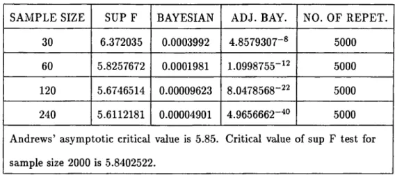
The 5 % critical values obtained for Sup F, Bayesian and Adjusted Bayesian tests

by the above procedure can be seen in the second, third and fourth columns of table

1 respectively. Andrews (1990), found the asymptotic critical value for Sup F test as

5.85 for 5% significance level. From table 1, it can be seen that the critical value that

we find for sample size 2000 is 5.8402522 which is very close to Andrews’ asymptotic value.

5.3 Finding The Powers of the Tests

After the first step o f finding critical values, the second step is finding the powers of the

tests. As stated before, the power o f a test can be defined as the probability of rejecting

the null hypothesis when the alternative hypothesis is true. Then what is needed to be

done is to define an alternative hypothesis and then to find the value of statistic under

that alternative hypothesis and finally compare that value with the critical value in order

to decide whether to reject the nuU hypothesis or not. Repeating this procedure a number

power of the test.

Then, on the way to obtaining powers the first step is to form the alternative hypothesis.

Firstly, we consider the case where there is no heteroskedasticity. There are two things to

decide on. The first one is the place of the change point. In this study, tw^o different change

points are considered, ^ X T and | x T. Secondly, the values o f regression coefficients, /?i

and /?2, are to be decided on. The noncentrality parameter denoted by 6 covers both of the things to decide on where it can be given as

— (/^1 “ + i^[T-t*]^[T-t*]) ) (01 ■” /^2) (69)

For this reason, it is appropriate to obtain power curves by finding the power for each

value of 6. As can be seen, i = 0 /?i = /?2· Then, for a fixed change point, 8

equals to zero means there is no structural change at the given point implying that power

equals to the significance level. As the difference between /?i and /?2 increases the value

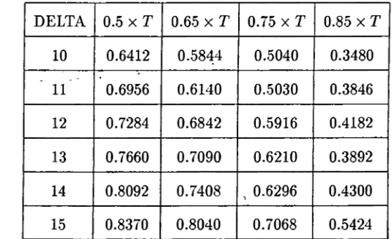
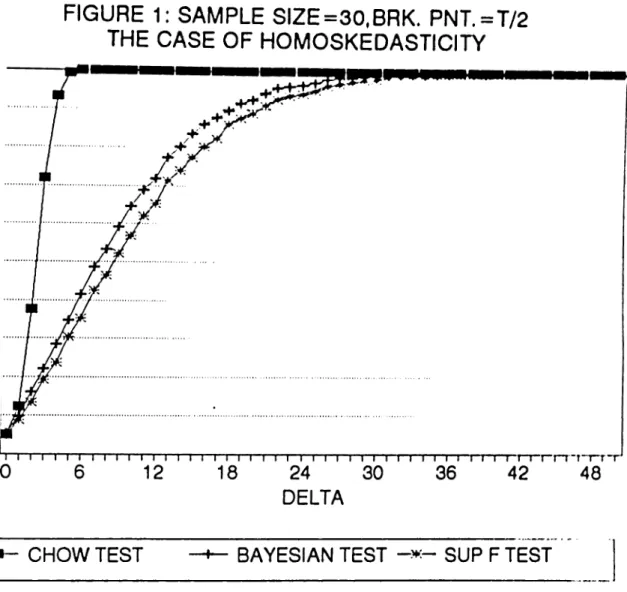
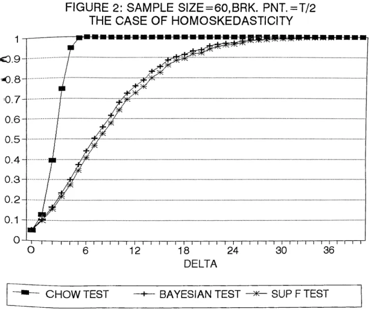
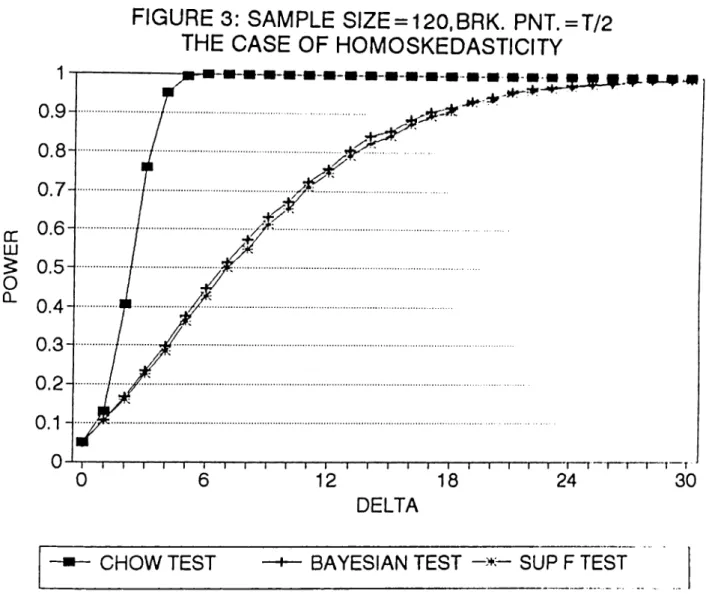
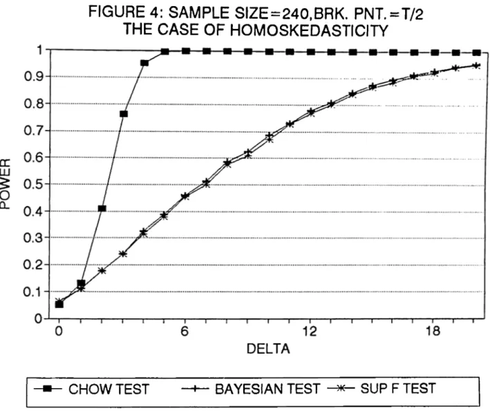
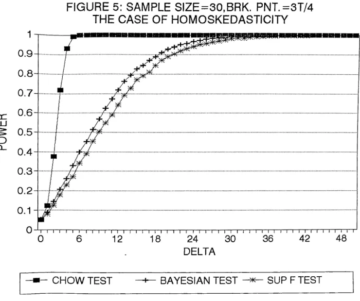
o f 6 will also increase implying an increase in power since the alternative hypothesis gets stronger with coefficients o f parameters apart from each other. In figures (1) to (20), the

power curves can be seen where on the horizontal axis there is 8 (where 8 ranges between zero and some value depending on the sample size ) and on the vertical axis there is power.

When there is heteroskedasticity, the change o f variance must also take place while

forming the alternative hypothesis. In this Monte Carlo study, we assume that for each

8 variance changes from one to two while moving from one regime to the other as can be seen from the model in section (5.1). In this case, i = 0 does not mean that the alternative

hypothesis coincides with the null hypothesis because under null hypothesis variance is

^The upper value of 6 decrease as the sample size increase cis can be seen from the figures. With high sample sizes it takes a long time for computer to compute powers and since as S increase powers get close to one asymptotically, the powers obtzdned for high values of 6 are not that important. As a result, in order to save time we decided not to obtain powers for high values of 8 when the sample size is large.

constant over the whole data but ^ = 0 does not mean a stable variance. As a result,

when (5 = 0 power of the tests does not equal to the significance level. This can be seen

in figures (9) to (14).

As stated in section (3), Chow test has F distribution . There is a special command in

Gauss which gives the area under the F distribution up to a given point. The things to be

given as inputs are degrees of freedom and noncentrality parameter. In this Monte Carlo

study to find the power of the Chow test we firstly get the critical value for 5 % from the F distribution tables. Then, we give degrees of freedom and noncentrality parameter

as inputs to the computer. Then computer forms the distribution under the alternative

hypothesis ( if w^e give i = 0, then it is under the nuU hypothesis ) and finds the area

up to the given critical value. One minus this area gives the probability o f rejecting the

alternative hypothesis so it gives the power o f the test. We repeated this for different

values o f delta and for sample sizes 30, 60, 120 and 240 in order to find the power curves.

In figures (1) to (8) the curves can be seen.

The procedure to find the powers of the Sup F, Bayesian and Adjusted Bayesian tests

given some change point t* and some S = 6o can be described as follows:

1. Form a Tx2 matrix o f independent variables X as given in section (5.1).

2. Generate randomly /?i and /?2 such that 6 = 6q given the change point t*.

, 3. Generate randomly a T x l vector o f error terms e which is distributed normally with mean zero and variance one under the assumption of homoskedasticity. Under the

assumption of heteroskedasticity generate randomly a T x l vector o f error terms 6[^*]

which is distributed normally with mean zero and variance one for the first part of

the data and generate randomly a (T - /* )x l vector of error terms which is

distributed normally with mean zero and variance two for the second part o f the

4. Obtain the dependent variable Y as below

Y =

_X[T-t*]p2. + €

when there is the homoskedasticity assumption. Obtain the dependent variable Y

as below

Y = 4 -₁ ■ f [ i * ] ■

when there is heteroskedasticity assumption.

5. Calculate the statistics o f (65), (67) and (68) for the tests Sup F, Bayesian and

Adjusted Bayesian respectively with the data Y and X .

6. Repeat (3)-(5) a number of times which is the Monte Carlo sample size. Then, a

M CSSxl vectors of Sup F, Kq and Kq values will be obtained. Calculate the number o f times each value is greater than the critical value obtained for each test. Then

divide this number to the Monte Carlo sample size in order to obtain an estimate of

the probability of rejecting the null hypothesis.

Repeating this procedure for different values o f starting from <5 = 0 and increasing

it , the power curve of the tests can be found. In figures (1) to (4) the power curves

of Sup F and Bayesian tests for the assumed alternative change point o f ^ x T and

T = 30,60,120,240 can be seen. In figures (5) to (8) the power curves o f the tests, this time for the assumed alternative change point of | X T and for same sample sizes, can

be seen. In each o f them there is the assumption o f homoskedasticity. The MCSS for each

o f the four sample sizes is 5000. Figures (9) to (14) are found under the assumption of

heteroskedasticity. The power curves of Adjusted Bayesian test, Bayesian test and Sup F

test can be seen. Figures (9) to (11) are for the assumed alternative change point o f | x T

for T = 30,60,120. In figures (12) to (14) the power curves this time for the assumed alternative change point o f | x T with same sample sizes as above can be seen. The

homoskedasticity and show the power curves o f Sup F, Bayesian and Adjusted Bayesian

tests. The first three of them assume the alternative change point as ^ x T and the last

three o f the assume alternative change point as | x T.

5.4 Comparison of Tests

In this section, some comparisons between the tests are made. Firstly, a power comparison

is made in order to find out how much we loose from not knowing the change point. As

stated in chapter (3), this loss can be found by comparing the power o f the test which

considers the change point endogenously with the power of the Chow test where change

point is assumed to be known. In our case, powers o f the Sup F test and Bayesian test

are compared to the power o f the Chow test. In figures (1) to (8), we see that power

curves o f Chow test are higher than the power curves o f both Sup F test and Bayesian

test as expected. What we do is to take the difference between power o f Chow test and

the powers of the Sup F and Bayesian tests for each 6, Then, we take the maximum of these differences so that we can indicate the loss from not knowing the change point by

this maximum difference.

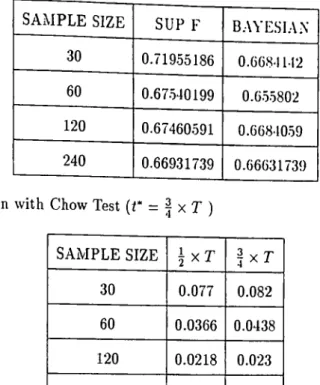
In table 2, the losses from not knowing the change point for the assumed alternative

change point of ^ x T can be seen. In second column of the table, the losses from not

knowing the change point for Sup F test can be seen. The loss is highest for sample size

30 and it decreases as the sample size increases. It starts with a maximum loss o f around

69 % and diminishes to a maximum loss o f around 64 % as we move to sample size 240. In the third column o f the table there are the losses from not knowing the change point for

Bayesian test. The losses for Bayesian test are lower than the ones for Sup F test for each

sample size. It starts with a maximum loss of around 65 % and diminishes to a maximum

more powerful test than the Sup F test. The maximum losses for each test seem to get

closer as the sample size increases leading one to think that the two tests converge to each

other.

In table 3, the losses from not knowing the change point for the assumed alternative

change point of | x T can be seen. Once again, the maximum loss is more for the Sup

F test for each sample size implying that Bayesian test is more powerful. Comparing

the results given in table 2 and table 3, we see that the maximum losses increased as we

changed the assumed alternative change point from ^ x T to | X T for both o f the tests.

This coincides with the results of Andrews (1990) for Sup F test since there it is written

that the power o f Sup F test is greatest when change occurs in the middle of the sample

and lowest when it occurs early or late in the sample.

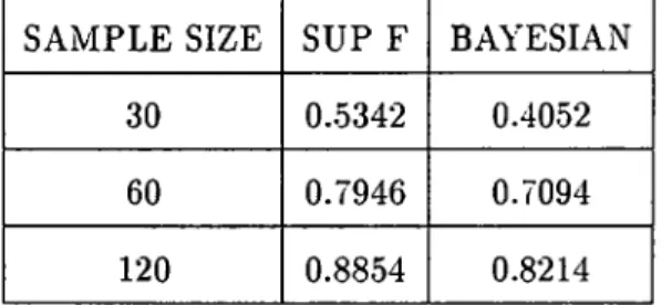
A better way to see which test is more powerful is o f course to compare their powers

with each other. From figures (1) to (8) we can see that the power curves o f the Bayesian

test is higher than the power curves of the Sup F test. Also, in table 4, there exists the

maximum o f the differences in powers of the Bayesian test and the Sup F test. In the first

column, we can see the maximum of the differences for the assumed alternative change

point o f I X T. For each sample size Bayesian test is more powerful than the Sup F test

but there is a decrease in difference as the sample size increase. This indicates that as

the sample size increase the two tests converge to each other but for small sample sizes

Bayesian test gives better results. Same kind o f results appear for the assumed alternative

change point o f | x T, which can be seen in the second column o f table 4. Once again

Bayesian test is more powerful than the Sup F test and also the two tests converge to each

other. Comparing the results o f the two cases we see that Bayesian test is more powerful

for the change point of | X T for each sample size. This implies that Bayesian test is even