The impact of uncertainty on investment : overview

THE IMPACT OF UNCERTAINTY ON INVESTMENT: OVERVIEW A Master’s Thesis by ERDAL YILMAZ Department of Economics Bilkent University Ankara September 2009

To my parents, especially to my brother Dr. Akın YILMAZ, his son A. Baran and, his daughter Yağmur.

THE IMPACT OF UNCERTAINTY ON INVESTMENT: OVERVIEW

The Institute of Economics and Social Sciences of

Bilkent University

by

ERDAL YILMAZ

In Partial Fulfillment of the Requirements for the Degree of MASTER OF ARTS in THE DEPARTMENT OF ECONOMICS BĐLKENT UNIVERSITY ANKARA September 2009

I certify that I have read this thesis and have found that it is fully adequate, in scope and in quality, as a thesis for the degree of Master of Arts in Economics.

--- Asst. Prof. Dr. Taner Yiğit Supervisor

I certify that I have read this thesis and have found that it is fully adequate, in scope and in quality, as a thesis for the degree of Master of Arts in Economics

---

Assoc. Prof. Dr. Fatma Taşkın Examining Committee Member

I certify that I have read this thesis and have found that it is fully adequate, in scope and in quality, as a thesis for the degree of Master of Arts in Economics.

---

Asst. Prof. Dr. Ebru Güven Solakoğlu Examining Committee Member

Approval of the Institute of Economics and Social Sciences

--- Prof. Dr. Erdal Erel Director

ABSTRACT

THE IMPACT OF UNCERTAINTY ON INVESTMENT: OVERVIEW

Yılmaz, Erdal

M.A., Department of Economics Supervisor: Asst. Prof. Dr. Taner Yiğit

September 2009

Common consensus in the real option literature is that there is a negative relationship between uncertainty and investment. One of the explanations can be stated that the increased in uncertainty leads to move up the value of waiting and consequently has an adverse effect on investment. Contrary to the existing theory, Sarkar (2000) and Gryglewicz et all (2006) find that this negative relationship is not always correct. The former paper demonstrates that an increase in uncertainty can actually hasten the probability of making an investment under certain condition (when project life is short and level of uncertainty is low) and hence uncertainty has a positive effect on investment. Result of the latter paper is exceptional in the sense that uncertainty may accelerate irreversible investment without building on the convexity of the marginal product of capital. In this thesis, we compare these two papers and investigate whether they support each other or not in the framework of real option theory. Moreover, we made some numerical simulations in order to understand clearly impact of other variables on investment along with uncertainty.

ÖZET

BELĐRSĐZLĐĞĐN YATIRIMLAR ÜZERĐNE ETKĐSĐ: GENEL BĐR BAKIŞ

Yılmaz, ERDAL

Yüksek Lisans, Ekonomi Bölümü Tez Yöneticisi: Yrd. Doç. Dr. Taner Yiğit

Eylül 2009

Reel opsiyon yazınında genel kabul görmüş görüşlerden biri, yatırımlarla belirsizlik arasında ters yönlü ilişki olduğudur. Belirsizlikteki artışın opsiyonun bekleme değerini artırarak yatırımlar üzerinde azaltıcı etkiye yol açtığı, bu duruma getirilen açıklamalardan biridir. Varolan yazının aksine, Sarkar (2000) ve Gryglewicz vd (2006) belirsizlik ve yatırımlar arasındaki negatif ilişkinin her zaman doğru olmadığını bulgulamışlardır. Birinci çalışma bazı koşullar altında (kısa ömürlü projeler ve belirsizliğin sınırlı olduğu) aslında belirsiziliklerin yatırm yapma olasılığını hızlandırdığını göstermiştir. Sermayenin marjinal hasılasının dışbükey olmaksızın bile belirsizliklerin yatırımları hızlandırabileceği bulgusu ikinci çalışmayı yatırım ve belirsizlik yazınında benzersiz kılmaktadır. Bu tezde, bu iki çalışmanın sonuçları karşılaştırılmakta ve birbirlerini destekleyip desteklemediği reel opsiyon çerçevesinde araştırılmaktadır. Belirsizlikle birlikte diğer değişkenlerin yatırım üzerine etkisini daha iyi anlayabilmek için çalışma bazı simülasyonlarla desteklenmiştir.

TABLE OF CONTENTS ABSTRACT ... iii ÖZET ...iv TABLE OF CONTENTS ...v CHAPTER I:

INTRODUCTION

...1

CHAPTER II:

REVIEW OF THE THEORIES FOR UNCERTAINTY AND

INVESTMENT

...5

CHAPTER III:

ILLUSTRATION OF PRICE UNCERTAINTY FOR

LASTING TWO PERIODS IN THE CONTEXT OF NET PRESENT

VALUE (NPV) AND REAL OPTION

...12

CHAPTER IV:

METHODOLOGY: CONTINGENT CLAIMS ANALYSIS

....20

CHAPTER V:

ECONOMIC ANALYSIS OF THE NON-MONOTONICITY

RESULT

...31

5.1 Economic interpretation of the impact of uncertainty on investment...31

5.2 Consistency of Parameters ...35

CHAPTER VI:

CONCLUSION

...39

SELECT BIBLIOGRAPHY

...41

CHAPTER I

INTRODUCTION

The neo-classical theory of investment emphasizes the importance of simple net present value (NPV) rule. According to this rule, a firm should invest in a project as long as the NPV is positive. That is, the present value of the expected stream of revenues that this project will generate should be greater than its cost. However, the classical theory neglects three main characteristics associated with investment decision, namely, irreversibility, uncertainty, and timing of investment. These characteristics imply that a firm can postpone investment to obtain more information about future. The possibility of delaying an irreversible investment project can lead to better investment decisions. This is the main theme of “the real option” approach, which was first developed by McDonald and Siegel (1986). The standard theory of the real options approach to investment is clearly explained in Dixit and Pindyck (1994). Moreover, in this `real options” approach, the investment opportunity (wait to invest) plays important role for investing a new projects and is viewed as an option to invest, which must be exercised optimally.

For an infinite-horizon setting, this policy can be described as follows: a firm should invest if the level of revenues (or NPV of project), say Q, exceeds some critical value Q*. This critical value Q*, naturally hinges on the parameters of the economy, particularly the level of uncertainty or the volatility of the project being considered. In terms of option theory, the investment rule can be equivalently stated as follows: a firm should invest when the value of the project is equal to its cost plus the opportunity cost of investing now. In the financial options literature, it has been shown that a higher level of uncertainty increases option value, and this leads to a more distant critical value for option exercise (for American options). Consistent with this intuition, the real options literature also predicts a negative relationship between uncertainty and investment, since greater uncertainty increases the value of the option to wait. As pointed out by Sarkar (2000), one finds repeated references to the negative investment–uncertainty relationship in the literature. He gives some examples:

“…this leads to the important implication that an increase in uncertainty raises the option value and thereby discourages new investment” (Mauer and Ott, 1995, p. 582); “…the recent literature on irreversible investment has shown that increase in uncertainty lowers investment” ( Caballero, 1991, p. 279);

and “…based on previous findings by researchers of an inverse relationship between uncertainty and investment” ( Metcalf and Hassett, 1995, p. 1472). Thus the general prediction of the real options literature is that a higher level of uncertainty will have a negative effect on investment.

Contrary to existing literature, Sarkar (2000) and Gryglewicz et all (2006)

claim that investments may be accelerated by increased uncertainty. They show that this particularly happens at low levels of uncertainty and when project life is short. Gryglewicz et all (2006) examine the impact of uncertainty on investment in three categories; discounting effect, volatility effect, and convenience yield effect. The first effect is related to discount rate via the risk premium component. Increase in uncertainty raises the discount rate, which results in reducing the net present value (NPV) of the investment and thus raises the investment threshold. The second effect is related to the value of the option to wait. In a sense that higher uncertainty increases the upside potential payoff from the option, leaving the downside payoff unchanged at zero (since the option will not be exercised at low payoff values). This increased option value implies that the firm has more incentive to wait, which also increases the investment threshold. Last effect author called convenience yield effect. The increase of asset riskiness raises the discount rate and thus also the conveniences yield of the investment opportunity. This decreases the value of waiting, so that it is more attractive to invest earlier resulting in a lower investment threshold. The contribution of this paper is related to the last channel of impact. It will be shown that last effect can in fact dominate, under some special condition; the first two affects and therefore uncertainty can speed up investment in case the uncertainty level is low and the project life is short1. So, changing the project life from infinite to finite can imply a negative

1

Sarkar (2000)analyzes the effects of the various parameters on investment and uncertainty relationship. Sarkar’s arguments can be summarized (i) the current level of uncertainty (σ) is low, (ii) the market price of risk (λ) is high, (iii) the correlation of return of the project with the market

relationship between uncertainty and the value of waiting, which reverses the basic real options result. Last but not least, this paper also supports Sarkar (2000) papers arguments, namely: the uncertainty–investment relationship is more likely to be positive when (i) the current level of uncertainty σ is low, (ii) project life (T) is short.

After giving brief introduction, the structure of my thesis will be as follows. In the next section, we will focus on related literature in order to show the importance of these two papers. This is followed by illustration example of NPV and real option. In the fourth section, we will solve this differential equation subject to the value matching and smooth pasting conditions at the investment trigger Q* and a zero value condition at Q=0. The derivations are standard and are omitted in these papers. We would like to emphasize the contingent claim analysis as a methodology used in real option and economic analysis of the non- monotonic results. Then we would like to check consistency of parameter that used in numerical example and make a comparison between Gryglewicz’s et all (2006) paper and Sarkar’s (2000) paper. In addition to this, we will make some numerical simulation in order to observe the impact of other variables on investment. Last part, we can conclude and propose some recommendation for future research topics and give way to our limitations.

in Q (µ) is low, and (vi) project life (T) is short. He also finds that the trigger Q* is always an increasing function of σ, as predicted.

CHAPTER II

REVIEW OF THE THEORIES FOR UNCERTAINTY AND

INVESTMENT

The decision of firms for investment is one of the important issues in economic literature. In particular, how firms form their decision under uncertainty has been investigate intensively in the literature since last two decades. The following chapter will be explored on the literature that looks at the relationship between investment and uncertainty. We will also incorporate this literature with the papers that we compare. Therefore, we will present a review and a discussion of the literature taking into account investment and uncertainty with the different strand.

There is no consensus on the exact nature of the relationship between investment and uncertainty. In general, different effects of uncertainty are highlighted by distinct theories. Some theories demonstrate the negative relationship and some theories present evidence for a positive one. According to Leahy and Whited (1995), investment under uncertainty has two dimensions. First,

they make a distinction between theories that analyze the firm in isolation and emphasize the variance in the firm’s environment. The authors focus on the theories that investigate the firm in relation to other firms and stress the covariance in returns between investment projects. With regard to the first theories, uncertainty itself plays key role for investment, whereas in the latter case uncertainty matters only if it affects covariance. Second, they can make a distinction between theories that claim that the marginal revenue product of capital (MRPC) is convex in some random variable, and theories that predict MPRC is concave. In contrast with the latter case, in the former case high variance of the random variable will encourage investment. In all of the theories that explore the impact of uncertainty on investment, covariance plays a key role. The importance of covariance investigated by Craine (1998) in the context of capital asset pricing (CAPM). According to CAPM

) ) ( ( ) (R_i R_{f i} E R_M R_f E = +β − where; ) (R_i

E is the expected rate of return on investment,

f

R is the risk-free rate of interest such as central bank interest rate,

i

β

is ( the beta coefficient) is the sensitivity of the investment returns to market returns, or also

) ( ) , ( M M i i R Var R R Cov =

β

, ) (RM

E(R_M)−R_f is sometimes known as the market premium or risk premium (the difference between the expected market rate of return and the risk-free rate of return.

The expected rate of return on an investment should be positively related to that investment’s risk, which, in turn, is measured by numerator of

β

_i (the covariance of its returns with the market as a whole). The higher covariance is the higher the riskiness of investment, an increase the expected rate of return on investment and reducing the level of capital stock. The CAPM predicts that the greater the covariance of returns the less the incentive to investment.

In general, firms invest less in the times when there is high uncertainty, that is, uncertainty discourages investment decision. The seminal papers of Brennan and Schwartz (1985), McDonald and Siegel (1986) and Paddock, Siegel and Smith (1988) were pioneer to build up an innovatory approach to the investment under uncertainty problem. This approach indicates the weakness of the NPV criterion for investment decision and suggested the view of an investment as a real option, analogous to the financial option theory of Black, Scholes and Merton (1973). The conclusion of the early models was that the uncertainty plays an important role— much more important than that of the discount factor in the NPV model—in investment decision making. The opportunity cost—the value of waiting to invest—raises the investment threshold and thus, depresses actual investment.

As also stated in the introduction chapter, the criterion for investment can be determined by the NPV approach. If NPV is positive then firms can take an investment decision. The NPV principle leads to two approaches. The first

followed Jorgenson (1963) compares the per-period value of capital marginal product and the per-period user costs that can be calculated from the input price, interest rates, and applicable taxes. The second, formulated by Tobin (1969), compares the capitalized value of the marginal investment to its replacement cost. However, the opportunity to delay project and irreversibility of investment make the model based on NPV criterion incorrect. After incorporating uncertainty in assessing irreversible investment in natural resources, Brennan and Swartz (1985) used the option pricing theory built up by Black and Scholes and Merton (1973). McDonald and Siegel (1986) identified the value of delaying the irreversible project when there is an uncertainty and they found the optimal timing of such investment. Real option framework for assessing the natural resources assets is developed by Tourinho (1979) and Paddock, Siegel and Smith (1988). Since then, the real options literature has grown. An outstanding survey and collection of theoretical models is investigated in Dixit and Pindyck (1994). Schwartz and Trigeorgis (2004) present a wide-ranging collected works of classical and recent theoretical papers.

The main assumption of real options model for the stochastic variable (such as project value) is based on a geometric Brownian motion (GBM) process. In order to describe long-term equilibrium, mean-reverting processes are more suitable contrary to GBM. A GMB process as an approximation of a mean-reverting process is examined by Metcalf and Hassett (1995). They argue that mean reversion has two opposing effects on investment under uncertainty: Mean reversion not only reduces the probability of reaching the investment threshold but

also investment threshold itself. Sarkar (2003) supports that the two effects cancel out only if the project’s risk is not correlated with the market or/and investors are risk neutral. By introducing systematic risk into the Hassett and Metcalf (1995) model, Sarkar (2003) showed that a geometric Brownian process cannot approximate a mean reverting process, and that the speed of mean reversion has effect on the probability of investing (and the investment-uncertainty relationship). Sarkar demonstrates that mean reversion will increase the project value and will decrease the option value under the assumption that revenues are stochastic. Thus, mean reversion will increase the probability of investing and will alleviate the investment-uncertainty relationship.

According to Antoshin (2006), the studies of Zeira (1990) and Nakamura (1999) indicate that a high level of firm risk aversion reinforces the negative effect of uncertainty on investment. On the other hand, a firm can be risk-seeking if the potential losses are small. This means that the investment-uncertainty relationship is positive at times of low uncertainty. This argument is also supported by Gryglewicz, Huisman, and Kort (2006). By accounting for systematic risk, Sarkar (2000) shows that uncertainty increases both the investment threshold and the probability of hitting the investment threshold. He suggests that for low-growth small firms, whose risk is highly correlated with the market, the investment-uncertainty relationship can be positive at times of low investment-uncertainty. In addition, French and Sichel (1993) suggest that firms can treat negative and positive shocks asymmetrically. If negative shocks prevail at times of high uncertainty and

positive ones at times of low uncertainty, uncertainty effects are opposite under low and high uncertainties.

Literature on capital imperfections does not explicitly incorporate uncertainty into the models. On the other hand, nearly all-real option models assume that the firm has unlimited access to finance resources. One of the rare attempts to bring these two lines of research together is made in Boyle and Guthrie (2003). They assign uncertainty not only to project value, but also to cash flows and allow external financing to be a notable proportion of the project value. In the framework of their real option model, cash has two opposite effects on investment: 1) a larger amount of cash enables realization of a larger number of investment opportunities; 2) under uncertainty, a heightened level of cash increases the value of waiting because the funds will still be available in the future. Thus, in the presence of cash flow uncertainty, liquidity has an ambiguous effect on the investment-uncertainty relationship: low liquidity depresses investment under uncertainty even further, through the costs of borrowing, and at the same time, low liquidity persuades the firm to take the investment opportunity now, because the prospects of project financing in the future are uncertain as noted by Antoshin (2006).

Bar-Ilan and Strange (1996) analyze the effects of investment lags. With respect to them, these lags lessen the disincentive effect of uncertainty on investment and tend to reduce inertia. For some parameter values, an increase in uncertainty can actually accelerate investment, a result contrary to that found in papers without investment lags. The policy implications of their results are worth

to discuss: projects with different investment lags respond to uncertainty differently. With a short lag, an increase in uncertainty delays investment. Thus, the volatility of the economic environment is a significant impediment to investment. They show that with a longer lag, an increase in uncertainty may encourage investment.

In the following chapter we will give an example in order to understand intuitively basic concept of NPV and real option.

CHAPTER III

ILLUSTRATION OF PRICE UNCERTAINTY FOR LASTING

TWO PERIODS IN THE CONTEXT OF NET PRESENT

VALUE (NPV) AND REAL OPTION

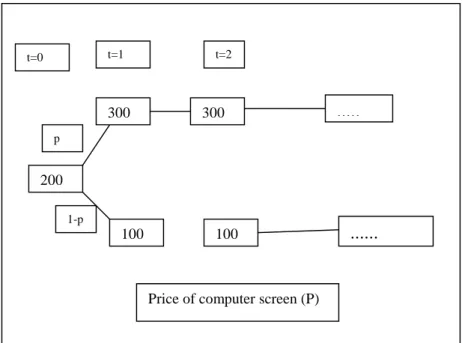
2

In order to understand the real option, it is a good starting point to examine a firm that is trying to decide whether to make an investment in a computer screen factory. One of the investment decision characteristics is irreversibility that means the factory can only produce computer screen, and should the market for computer screen vanish, the firm can not disinvest and consequently the expenditure are sunk costs. Hence the firm is not able to recover its expenditure. Dixit and Pindyck (1994) assume without loss of generality that the factory can be built instantly, at a cost I, and will produce one computer screen per year forever, and the operating cost is zero. This assumption also implies that the project generates a steam of cash flow equals to the price of output. At time 0, the price of computer screen is $200, but the following year it is assumed that price will change upward and downward with an equal probability (p=0.5). Therefore, with probability p, price

2

of computer screen will go up to $300, and with probability (1-p), it will fall to $100. The price will then remain at this new level forever (see Figure 3.1). The probabilities of price (p) change and factory cost (I) are important determinants of investment decision. We will see this later.

Figure 3.1: Price of Computer Screen

The additional assumption that they make is to assume that risk over future price of computer screen is completely independent from what happens the overall economy. Consequently, the firm should take risk-free interest rate in order to discount future cash flows, and they assume that risk-free interest rate is 10 percent.

In order to illustrate concept of NPV and real option, they assume that

I=$1600 and p=0.5. It is worth to raise the question that this is a good investment

given these values. Should the firm invest now, or would it be better to wait a year and see whether the price of computer screen goes up or down? Suppose

200

300

100

300

Price of computer screen (P) 100 t=0 ... ... t=1 t=2 p 1-p

investment decision is taken to invest now. Calculating the net present value of this investment in the standard way. Furthermore, the expected future price of computer screen is always $200 in our example.

(

1

)

( ) 0,5*300 0,5*100 $200 ) ( ) ( 1 1 1 = + + − + = + = + t DOWN UP t t P pE P p E P E 600 $ 2200 1600 ) 1 . 0 1 ( 200 -1600 NPV0 0 = + − = + + =

∑

∞ = t t

(1)

It appears that the NPV of this project is positive((NPV=)$600>0). The current value of computer screen factory, which they denote by V0, is equal to $2200, which exceeds the $1600 cost of the factory. According to NPV, theory the future cash flows of an investment project are estimated and if there is uncertainty about those cash flow the expected value determined. The expected cash flows are discounted at the cost of capital for the corporation and the results summed. If the NPV is positive the project is worthwhile and should be pursued. If it is negative the project should be turned down. If the NPV is zero it does not matter to the corporation whether the project is accepted or rejected. Therefore, a firm considered in our case should invest.

The conclusion drawn above is incorrect, since it ignores one of the main characteristics of investment, timing of investment. In other words, the computations above disregard a cost -the opportunity cost of investing now, rather than waiting and keeping open possibility of not investing should the price fall. In order to make it clear, let us make above computation for the NPV of this project a second time, rather than investing now, a firm will wait one year and then makes

an investment if computer screen price increases (price of computer screen =$300, noting that only investing if price of computer screen increases is in fact ex-post optimal). NPV turns out to be calculated as follows:

773 $ 1 . 1 850 ) 1 . 0 1 ( 300 ) 1 . 0 1 ( 1600 ) 5 . 0 ( 0 1  = =      + + + − =

_∑

∞ = t t NPV (2)

It is worth to note that in year 0 above example, there is no investment; consequently there is no revenue and no expenditure in year 0. In the next year, in case only price rise to $300, the $1600 is spent. This happens with probability 0.5. Therefore, if a firm waits a year before taking the decision on whether to invest in the factory, the project’s NPV today is $773, whereas it is only $600 if a firm invests a year 0. It is obvious that it is better to wait a year than to invest year 0.

Note that if a firm’s only choices were to invest today or never invest, a firm invests today in above example since NPV is positive. In that case there is no option to wait a year, hence no opportunity cost to kill such an option, so the standard NPV rule applies. Two things are needed to introduce an opportunity cost into the NPV computation – irreversibility, and the ability to invest in the future as an alternative today. The less time there is to delay, and the greater the cost of delaying, the less will irreversibility affect the investment decision.

How much is it worth to have the flexibility to make the investment decision next year, rather than having to invest either now or never? (a firm knows that having this flexibility is some of value, because a firm waits rather than invest now). The question is then what is the value of this ‘flexibility option’? The

answer is simple to calculate; it is just the difference between the two NPV’s, that is, NPV1- NPV0 ($773-$600= $173). Put it differently, the firm is ready to pay $173 more for an investment opportunity in case of flexibility instead of only invest now. In sum, the firm is better off waiting until next year to take a decision for investment. As it is shown by above example, two important of investment characteristics play a key role when a firm makes an investment decision, irreversibility and possibility to postpone. Furthermore, above example also indicates the weakness of standard neoclassical investment model (NPV value approach). This can be explained due the fact that irreversible investment opportunity is much like a financial option, that is, a firm has an opportunity to invest holding an ‘option’ that is analogous to a financial call option. In sense that a call option gives the right but not obligation for some specified time (at some future time) to pay exercise price and in return buy an asset that has some value. Furthermore, exercising the option is also irreversible; despite the fact that an asset can be sold to another investor, one cannot recover the option or the money that was paid to exercise it. A call option to invest is valuable in part because the future value of an asset obtained by investing is uncertain. In this context, the investment rule can be equivalently stated as follows: invest when the value of the project exceeds its cost by an amount equal to the option value of waiting to invest.

It is worthwhile to reexamine above example in the context of real option.

Let F1 be the value option next year. There are two possibilities of price

( )

1.1 $1700 300 1600 0 1 =− +

∑

= ∞ = t t F

However, in case of price fall to $100, the option is not exercised. It means 0

1 =

F . In order to compute the value of the option today F , we should form a 0

portfolio with two components: first component is the investment opportunity itself and second component has a certain amount of output. The portfolio is risk-free that assumption is needed for no arbitrage condition. Therefore, the value of the portfolio today can be computed as follows:

0 0 0 =F −nP

ϑ

Today price is P₀ =$200, and then the value of the portfolio today is

n F₀ 200

0 = −

ϑ

. In the same manner, the value of the portfolio for next year which depend on P1can be obtained:

1 1 1 =F −nP

ϑ

The next year price is $300 in case of P1 (goes up to), then

( )

1.1 $1700 300 1600 0 1 =− +

∑

= ∞ = t t F

Consequently,

ϑ

1a =1700−300n, if price went down to $100, then F1 =0, this

case implies that option is unexercised and hence

ϑ

_1b =0−100n=−100n.n is chosen such that the portfolio

ϑ

₁ is risk-free that means we should equate

b a 1 1

ϑ

ϑ

= : n n 100 300 1700− =− ,

From above equation, we get n=8.5. We can also calculate the value of the portfolio for next year is

850 5 . 8 * 100 1 =− =−

ϑ

, or ,

ϑ

₁ =1700−300*8.5=−850.

The value of the portfolio for next year in both cases (either price up or down) is –850. Before computing the capital gain of this portfolio, we should calculate the payment that must be received by the holder of short position (option premium). Return of this portfolio can be obtained as follows:

premium option

return

portfolio_ =

ϑ

₁−

ϑ

₀ − _

Since the expected price for next year is the same as current year ($200), and the price does not change over time, the expected rate of capital gain on computer screen is zero. No rational investor would be willing to hold a long position because of no capital gain in the long term. The holder of a long position should expect to receive at least 10 percent in order to hold long position. Therefore, selling computer screen short will require a payment of

(r*P₀ =0.1*200) $20 per computer screen per year. It is worth to note that this is analogous to selling short a dividend paying stock; the short position requires payment of the dividend, no rational investor will hold the offsetting long position without receiving that dividend. We obtained the short position of 8.5 unit of computer screen previously in our portfolio and we easily can calculate the option premium as follows 170 $ 5 . 8 * 20 * _

_ premium=required return n= =

It is time now to compute the capital gain of holding this portfolio over the year: premium option return portfolio_ =

ϑ

1−

ϑ

0 − _ 170 ) ( 170 _{1 0 0} 0 1 −

ϑ

− =

ϑ

− F −nP −

ϑ

170 200 * 5 . 8 850− ₀ + − − = F 0 680−F =

Since there is no arbitrage and the above return is risk-free, any capital gain must equal to 10 percent of the initial portfolio, that is,

) 1700 ( * 1 . 0 680−F₀ = F₀ −

We can obtain that F₀ =$773. That is the opportunity cost of investing today. It is also obvious that this is the same value that we determine before the computing the NPV of the investment under the assumption that we will follow the optimal strategy of waiting a year before deciding whether to invest. In the next section we will focus on computational technique used in real option, namely contingent claim analysis, in a greater detail.

CHAPTER IV

METHODOLOGY: CONTINGENT CLAIMS ANALYSIS

There are basically two techniques in the real options theory in order to calculate the value of waiting to invest (investment opportunity); dynamic programming and contingent claims analysis (Dixit and Pindyck[1994]). Although these two techniques are strongly associated with each other, and lead to yield identical outcome in many applications, two techniques differ from each other due to the fact that they have different assumptions about financial markets, and discount rates that firms use to value future cash flows according to Dixit and Pindyck (1994). Furthermore, the discount rate is determined endogenously as an implication of the overall equilibrium in capital markets in the contingent claims analysis (CCM) as compared to dynamic programming and hence CCM suggests a better dealt with the discount factor. To summarize why we prefer use of contingent claims analysis of real investment opportunities, the assumption of uncertainty affecting the discount rate and convenience yield appears to be the most plausible one. This arguments is parallel to Gryglewicz et all (2006).

On the other hand, one of the core assumptions in the CCM is that existing assets with a price that is perfectly correlated with Q so that uncertainty over future values of Q can be replicated by existing assets must span the stochastic variations in Q. With this assumption, CCM allows to make analysis the equilibrium impact of the systematic risk on the discount rate, and, on the value of investment option and, the investment policy by using the intertemporal CAPM of Merton (1973) as pointed out by Gryglewicz et all (2006). Using the spanning technique, let P be the price of the asset that is perfectly correlated with Q. Let

PM

ρ

be the correlation of P with market portfolio M, then,

ρ

_PM=

ρ

_QM. Since P is perfectly correlated with Q, P is assumed to evolve the same way:

t t t t Qdt Qdz dQ =

µ

+

σ

(3) t t t t Pdt Pdz dP =

π

+

σ

(4)

where µ is the drift parameter or the expected percentage rate of change in Q (the growth rate of Q),

σ

is the volatility (uncertainty) of the process and dz is _t

the increment of a standard Brownian Motion process which is log-normally distributed.

π

is risk-adjusted rate of return on this asset. By the Capital Asset Pricing Model (CAPM),

π

also reflects the asset’s systematic risk. The

π

is given by:

where

(

)

M

M r

r

σ

λ = − is the aggregate market price of risk. r_Mis the expected return on the market which can also be considered as return of the whole market portfolio that provides availability of diversification. r is risk-free interest rate and assumed to be exogenous. The risk premium is determined by the covariance between rM and r . It is assumed that

π

>µ in order to guarantee that

a firm makes invest in the project. Convenience yield of the investment opportunity is described as the difference between

π

, the expected return of the project, and µ, the expected percentage rate of change in Q. The difference is shown by δ or put it differently, which is an opportunity cost of delaying investing in the project and keeping the option to invest alive. And therefore, δ satisfies:

µ

σ

λρ

µ

π

δ

= − =r+ PM − (6)

In case of δ =0, that is π =µ, then this implies that there would be no opportunity cost to keeping the option alive, and the firm never invest in this project. Therefore, it is worth to analyze the case where δ >0, which is said before this assumption ensures that the investment is ever undertaken; otherwise it is never optimal to exercise the option. We will make this point more clear later. The level of uncertainty faced by the firm is measured by the volatility parameter

σ

. From (6) we obtain that a change in σ results in a change of

π

, which must lead to an adjustment of either µ or δ or both. In general, this relation depends on what is assumed to be an endogenous parameter affected by changes in volatility. A certain guideline in this respect could be Pindyck (2004), which relates commodity

inventories, spot and future prices and the level of volatility. The model is estimated for several commodities and the results show that a volatility shock has a significant effect on the convenience yield and only a small effect on the price. Consistent with this evidence, it also seems to be more common in the related literature on the investment–uncertainty relationship to assume that µ is fixed and δ changes with

σ

(e.g., [Sarkar, 2000] and [Sarkar, 2003]) as presented and pointed out by Gryglewicz et all (2006). We follow Gryglewicz et all (2006) assumptions.

It is also obvious under the above assumption that in case of δ is very large which implies the opportunity cost of waiting is large, thus the value option will be very small (from equation 6). Thus µ (the expected percentage rate of change in Q) then can be expressed as:

























=

Q

dQ

E

dt

*

1

µ

₍₇₎

and if we plug 7 into 6, δ can be expressed as a function of Q:

            − = Q dQ E dt Q) 1 * ( π δ (8)

It is worth to focus on the value of the project, denoted by V(Q), before

policy. The project value is a function of the stochastic revenues and changes over time and depends on the current realization of Q. The project value (V(Q)) can be

obtained by the expected present value of the revenue stream discounted by the risk-adjusted discount rate. If the project has a finite life of T years, then the project value at the time of the investment as formulated by Gryglewicz et all (2006) is

µ

σ

λρ

σ λρ µ π π − + − = =       = =

_∫

−

_∫

− − − + PM T r t T t t t T r e Q Qd e Q Q d Q e E Q V PM t ( ) 0 ) ( 0 0 1 ) ( ₍₉₎

Before the project is installed, the firm holds an option to invest. The option is held until the stochastic revenue flow reaches a sufficiently high level at which it is optimal to exercise the option and invest. The option value (F(Q)) can

be found by constructing a risk-free portfolio, determining its expected rate of return, and equating that return to the risk free rate of interest rate, r. To construct such a portfolio, consider holding an option to invest, which is worth F (Q).

Assume short position of N =F'(Q) units of the project. In order to compute value of this portfolio, we use standard approach (Dixit and Pindyck(1994), ch 5) 3 and the value of portfolio is given by:

) ( * ) ( ' Q F Q Q F w= − (10) dQ Q dF Q Q dF Q dF dw= ( )− '( )* − '( )* (11) 3

where dQ dF Q F'( )=

The composition of the portfolio will be changed from one short interval of time to the because of the fact that the portfolio that is constructed is a dynamic portfolio. However, over each short interval length dt , N is held as a fix.

This short position in this portfolio will require a payment of '( )

Q QF

δ

dollars to holder of the long position every time period. As the total expected return on the project that can be obtained from equation 6 is equal to expected rate of capital gain plus the dividend rate (π =δ +µ) and consequently an investor holding a long position in this option will claim the risk-adjusted return as follows:

3 2 1 3 2 1 3 2 1 gain capital stream dividend urn edtotalret riskadjust Q Q Q _ _ * * * δ µ π = + (12)

where δ*Qrefers to dividend stream and µ*Q the growth of the firm’s project (capital gain). On the other hand, the total return from holding the portfolio over a short time interval dt is given by

dt Q QF

dw−δ '( ) (13) If we plug equation (11) into equation 13 and, it is worth to note that we

assume that N =F'(Q) does not change over time dt , therefore, in the above equation the term dF'(Q)Q is omitted in the equation 11, therefore, we

get following expression;

dt Q QF dQ Q F Q dF( )− '( ) −δ '( ) (14)

In order to get an

expression for dF , it necessitates making use of Ito’s lemma:

2 '' ' ) )( ( 2 1 ) (Q dQ F Q dQ F dF = + (15) where 2 2 '' ) ( dQ F d Q F =

In order to get last term in equation 15, we take square of equation 3 and get the following equations:

(dQ)2 =(µQdt)2 +2µσdtdz+(σQdz)2 (16)

As dz is the increment of Wiener process and satisfied the following conditions:

And dz2 =dt, dt2 ≈0

Second term is also close to zero and it vanishes in the equation 16, therefore we end up: 2 2 ) ( ) (dQ = σQdz (17) or (dQ)2 =σ2Q2dt The total return on the portfolio can be expressed.

dt Q QF dQ Q F ( )( ) ( ) 2 1 '' 2 −δ ' (!8)

Again substituting equation 17 into 18,

dt Q QF dt Q F Q ( ) ( ) 2 1σ2 2 '' −δ ' (19)

In order to satisfy no arbitrage condition, equation (19) must be equal to

dt

Q

QF

Q

F

r

rwdt

(

=

(

(

)

−

'

(

))

. If we equate this expression with the total risk-free return on total portfolio, we get the following expression,

[

F Q QF Q

]

dt r dt Q QF dt Q F Q ( ) ( ) ( ) ( ) 2 1σ2 2 '' −δ ' = − ' (20)

Dividing both side of equation 20 by dt and

rearranging the above equation, which yields the second order differential equation that F (Q), must satisfy:

0 ) ( ) ( ) ( ) ( 2 1 2 2 '' + − ' − = Q rF Q QF r Q F Q δ σ (21)

F (Q) also satisfies the following boundary conditions: 0 ) 0 ( = F (22) F(Q*)=Q*−I (23) _F'_(Q*)=_{1 (24)}

Again Q represents value of the project at which it is optimal to invest* 4.

Condition (22) states that when Q=0, the value of the option to invest has no value. Equation (23) is the value-matching condition that is upon investing; the firm receives a net payoff Q*−I. Rewriting (23) as I =Q*−F(Q*) which implies that when the firm invests in the project, it gets the value Q , but gives up

the opportunity to investF(Q).

4

The critical value Q is obtained when this net gain * Q*−F(Q*) is equal to the direct cost of I (investment). Put it differently, the value of the project Q *

(Q*=I +F(Q*)) is set equal the direct cost of investment, I , plus the opportunity cost F(Q*) . Equation (24) is the smooth-pasting condition. That is, if F(Q)

were not continuous and smooth at the critical value Q , it is better for firm to *

wait t∆ to observe next step of Q . To solve for F(Q) we must solve equation 21 subject to the boundary conditions (22,23 and 24). McDonald and Siegel (1986) suggested that the solution that satisfies the condition (22) must take the form5:

β AQ Q

F( )= (25) Condition (23) and (24) can be used to solve for A which is a constant to be determined, and for optimal value of Q , * β is a known constant whose value depends on the parameter;

σ

, r and, δ of equation (21), where β >1.

To obtain value of A and Q , we substitute equation (24) into (23) and (24) so *

that I Q AQ Q F( *)= *β = *− (26)

And then, from equation 26, we get

β * * Q I Q A= − (27)

By equation (24), F'(Q)= AβQ*(β−1) =1, using (27) to substitute for A we obtain:

5 1 2 2 1 ) (Q AQβ A Qβ

F = + Since boundary condition (22) is F(0)=0 which implies that

. 0

2 =

1 * 1 _=      − Q I β or Q _I      − = 1 * β β (28)

Substituting (28) into (27) in order to obtain a value for A as

(

)

( ) (β ) β β β β β β ββ ββ ββ ββ 1 1 1 )) ) ) 1 ( (( ) 1 ) 1 ( ( )) ) ) 1 ( (( ) ) 1 ( ( − − − = − − − = − − − = I I I I I I A (29)

In order to find β, we should take the derivatives of equation 25 and we end up the following equations:

) 1 ( ' ) (Q = AβQ β− F (30) F''(Q)= Aβ

(

β −1

)

Q(β−2) (31)

If we plug, (30) and (31) into the second differential equation (equation 21), we end up with the following quadratic equation:

(

1

)

( ) 0 2 1 2 − + − − = r r δ β β β σ ₍₃₂₎

We are looking for the positive root (β >1) of quadratic equation 32 Then we obtainβ as follows in terms parameter,

(

)

(

)

(

(

)

)

2 _1. 2 1 2 1 2 2 2 2  >       +     − − + − + − + − − = σ σλρσ µ σλρσ µ β r r r r r (33) or

(

)

(

)

        +     − − + − − = ₂ 2 2 2 2 2 1 2 1 σ σ λρσ µ σ λρσ µ β r

        +     − ₋ + − − = ₂ 2 2 2 2 2 1 2 1 σ σ δ σ δ β r r r (34)

Therefore, β depends on value of the parameters;δ ,

σ

and, r . In general,

r is treated as a constant. Furthermore, we plug β in order to solve for Q* in equation 27 which yields the investment trigger:

(

)

r _e ( ) I Q λρσ_{r λρσ µ}µ_T ββ ₋ − + − − + − = 1 1 * (35) or

(

)

_e ( ) I Q δ _{δ T} ββ_{− −} − = 1 1 *

from equation 35, we can conclude that the investment trigger value hinges β,δ , r ,

σ

, and T. We will explore the relationship between trigger value of investment and relevant parameter in the following section. In particular, we are interested in more what the impact of change the level of uncertainty (

σ

) on investment.

CHAPTER V

ECONOMIC ANALYSIS OF THE NON-MONOTONICITY

RESULT

In this chapter will be related to economic analysis of non-monocity result and examining the consistency of the parameters and presenting results of our simulations.

5.1 Economic interpretation of the impact of uncertainty on investment

In this section, we will focus on and summarize Gryglewicz et all (2006). We also present an economic interpretation of the non-monotonic effect of uncertainty shown in (λρ >0). The investment trigger can be stated as

(

)

r _e ( ) I Q λρσ_{r λρσ µ}µ_T ββ ₋ − + − − + − = 1 1 *

At this point it is a good starting point to trace all the variables that are influenced by uncertainty and consider the trigger value as a function of two6 parameters: Q*(δ(σ),β(σ,δ). Then the derivative of the investment trigger with respect to σ can have three effects in the following way:

43 42 1 43 42 1 43 42 1 Effect yield e Convinienc Effect Volatility Effect g Discountin Q Q Q Q d d

σ

δ

δ

β

β

σ

β

β

σ

δ

δ

δ

σ

β

σ

δ

σ

∂ ∂ ∂ ∂ ∂ ∂ + ∂ ∂ ∂ ∂ + ∂ ∂ ∂ ∂ = * * * )) , ( ), ( ( * (36)

The three effects have a clear explanation and each has an unambiguous sign (for the case of λρ>0). The discounting effect, the first term on the right-hand side, is related to the impact of revenue uncertainty on the rate used to discount that affect the project value. An increase level of uncertainty leads to raise the discount rate via risk premium component, which decreases the NPV of the investment project. This means that it is less attractive or profitable to invest in this project, which ends up an increase of the trigger value. Therefore, it is concluded that the discounting effect is always positive.

Since the derivative of the trigger with respect to

β

has two effects due to fact

β

is a function of

σ

and δ . The first effect is called by Gryglewicz et all (2006) as volatility effect and second one is called convince yield effect. These two effects capture the impact of uncertainty on the value of the option to wait. According to Gryglewicz et all (2006), these two effects combined as the option

6

Since both

β

and δ depend on

σ

. The value of trigger investment is a function of three parameters.

effect. The volatility effect, which is characterized by the derivative,

σ

β

β

∂ ∂ ∂ ∂Q*

reflects the direct impact of uncertainty on the value of the option to wait. Higher uncertainty raises the upside potential payoff from the option, leaving the downside payoff unchanged at zero (since the option will not be exercised at low payoff values). This is the well-known positive impact of uncertainty on the option value with respect to Gryglewicz et all (2006) and Dixit and Pindyck(1994). A(n) decreased (increased) option value means that the firm has less (more) incentive to wait. This increases the opportunity cost of investing and consequently the investment trigger will increase. Hence, the effect is clearly positive.

The product

σ

δ

δ

β

β

∂ ∂ ∂ ∂ ∂ ∂Q*

in equation (36) reflects the influence of

uncertainty on the option value via the convenience yield that can be called as the convenience yield effect. Decreased uncertainty reduces the risk premium of the expected rate of return and thus also the convenience yield, which in turn drops the opportunity cost of holding the option and consequently increases its value. For this reason it is attractive to invest later, which raises the trigger.

All in all, from above discussion one can conclude that the convenience yield effect is negative, whereas the discounting and volatility effects are positive. It is obvious that, under the condition that if the convenience effect dominates the two other effects, one can observe the positive relationship between uncertainty and investment.

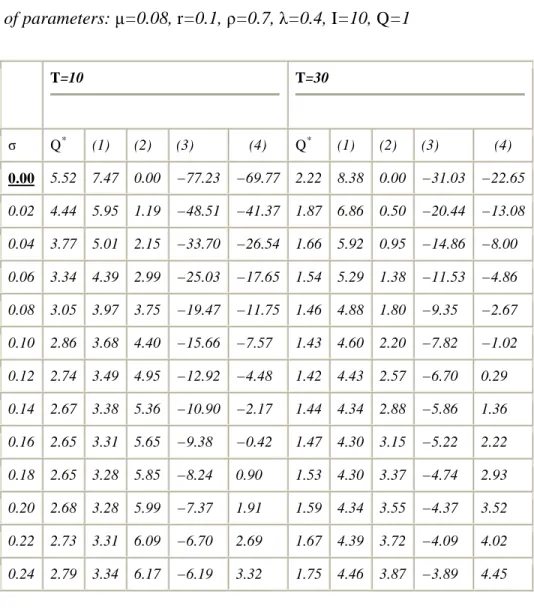
Table 5.1. The impact of uncertainty on investment

The three effects of uncertainty affecting the position of the investment trigger for the set of parameters: µ=0.08, r=0.1, ρ=0.7, λ=0.4, I=10, Q=1

T=10 T=30 σ Q* (1) (2) (3) (4) Q* (1) (2) (3) (4) 0.00 5.52 7.47 0.00 −77.23 −69.77 2.22 8.38 0.00 −31.03 −22.65 0.02 4.44 5.95 1.19 −48.51 −41.37 1.87 6.86 0.50 −20.44 −13.08 0.04 3.77 5.01 2.15 −33.70 −26.54 1.66 5.92 0.95 −14.86 −8.00 0.06 3.34 4.39 2.99 −25.03 −17.65 1.54 5.29 1.38 −11.53 −4.86 0.08 3.05 3.97 3.75 −19.47 −11.75 1.46 4.88 1.80 −9.35 −2.67 0.10 2.86 3.68 4.40 −15.66 −7.57 1.43 4.60 2.20 −7.82 −1.02 0.12 2.74 3.49 4.95 −12.92 −4.48 1.42 4.43 2.57 −6.70 0.29 0.14 2.67 3.38 5.36 −10.90 −2.17 1.44 4.34 2.88 −5.86 1.36 0.16 2.65 3.31 5.65 −9.38 −0.42 1.47 4.30 3.15 −5.22 2.22 0.18 2.65 3.28 5.85 −8.24 0.90 1.53 4.30 3.37 −4.74 2.93 0.20 2.68 3.28 5.99 −7.37 1.91 1.59 4.34 3.55 −4.37 3.52 0.22 2.73 3.31 6.09 −6.70 2.69 1.67 4.39 3.72 −4.09 4.02 0.24 2.79 3.34 6.17 −6.19 3.32 1.75 4.46 3.87 −3.89 4.45

The columns present: the discounting effect (1), the volatility effect (2), the convenience yield effect (3) and the total effect (4).

We reproduced Gryglewicz’s et all (2006) results using their method in the Table 5.1.The parameters that are used in the table taken from Sarkar (2000) He chooses these values for the following reason: ρ=0.7 reflects a projects imperfectly (but positively) correlated with market, he states that this number assigns for the

correlation is a description of the majority of the projects; and the market price of risk value (λ=0.4) is the approximate historical average (see Bodie et all., 1996, p.185). Risk-free interest rate,r is chosen as used by Dixit and Pindyck (2004),

µ

is chosen such that it must guarantee the condition δ >0.

It is worth to note that both discounting and volatility effect has positive sign independently from time horizon. The convenience yield effect is negative for all level of uncertainty that presented in our table for both short and long project life (T=10,30). However, the longer the project life, total effect takes only negative value for the low level of uncertainty. For example, when T=30, up to 0.1 level of uncertainty, total effect is negative and after this level, it turns out to be positive. This argument supports non-monotonic effect of uncertainty. Lastly, the trigger value of investment for short life project is lower than the long life of project. This finding also supports Sarkar (2000) in a sense that when project life is short, it is more likely to be positive relationship between investment and uncertainty.

5.2 Consistency of Parameters

In order to verify the consistency of parameters, we investigate the value that assign for parameters in Table 1 are consistent or not. In other words, we checked whether these parameters guarantee that and δ >0. We confirm that these parameters are consistent.

It is worth to note that we can obtain the value of

β

in previous section and we can calculate δ and

β

as follows

µ

σ

λρ

δ

=r+ PM − and        +     − ₋ + − − = ₂ 2 2 2 2 2 1 2 1

σ

σ

δ

σ

δ

β

r r r

We use above equations in order to verify consistency of parameters. For this purpose, we construct Table 5.2.

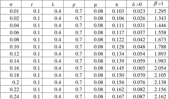
Table 5.2 Consistency of the model parameters

0

> −

=

π

µ

δ

, and,

β

>1 are the main assumption of the model. Hence it is important to verify whether the parameters that are chosen for numerical analysis satisfy

the main assumption. The assumptions are basically guaranteed that investment will

undertake. σ r λ ρ µ π δ >0

β

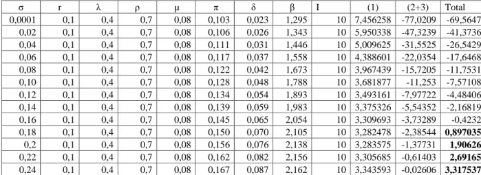
>1 0.01 0.1 0.4 0.7 0.08 0.103 0.023 1.295 0.02 0.1 0.4 0.7 0.08 0.106 0.026 1.343 0.04 0.1 0.4 0.7 0.08 0.111 0.031 1.446 0.06 0.1 0.4 0.7 0.08 0.117 0.037 1.558 0.08 0.1 0.4 0.7 0.08 0.122 0.042 1.673 0.10 0.1 0.4 0.7 0.08 0.128 0.048 1.788 0.12 0.1 0.4 0.7 0.08 0.134 0.054 1.893 0.14 0.1 0.4 0.7 0.08 0.139 0.059 1.983 0.16 0.1 0.4 0.7 0.08 0.145 0.065 2.054 0.18 0.1 0.4 0.7 0.08 0.150 0.070 2.105 0.2 0.1 0.4 0.7 0.08 0.156 0.076 2.138 0.22 0.1 0.4 0.7 0.08 0.162 0.082 2.156 0.24 0.1 0.4 0.7 0.08 0.167 0.087 2.162

Furthermore, we also check the consistency of the parameters which are not explored intensively Gryglewicz at all (2006). We construct Table 37 based on the value used by the authors. The results that we obtain from in Table 3 also verify the parameters that are chosen for numerical analysis satisfy the main assumption (

δ

=

π

−

µ

>0, and,

β

>1). We make another simulation in order to compare the Sarkar (2000) arguments with Gryglewicz at all (2006) methodology. For this purpose, we form the Table 4 (Appendix) According to Sarkar (2000) assumptions the uncertainty–investment relationship is more likely to be positive when (i) the current level of uncertainty σ is low, (ii) λ is high, (iii) ρ is high, (iv) r is high, (v) µ is low, and (vi) T is short. Taking these assumptions as a granted using Gryglewicz at all methodology, we choose the following parameters;

06 . 0

=

µ

, r =0.15,

ρ

=0.9, λ =0.7. The first thing should be worth to mention is that these two paper support each other. The difference comparing to Table 1 with Table 4 is the positive relationship between uncertainty and investment verified in the low level of uncertainty in Table 4 considered the Sarkar (2000) arguments. For example, it is important to note that up to 0.04 level of uncertainty in Table 4, we can observe positive relationship, whereas this positive relationship can be observed in Table 1 up to 0.1 level of uncertainty. Therefore, we can conclude that other variables also play important role impact of uncertainty on investment. Equally more important, the first effect (discounting effect) and β became convex function of uncertainty in Table 4. In table 5, we change the model basic parameters, (

µ

=0.04,r=0.05,

ρ

=0.01, λ =0.01) (by doing this,

we assume that the market price of risk and project return less correlated with market return and interest rate is so low, then

π

andδ became almost constant,

β

is a decreasing function of σ) and we observe that under new parameters when σ is close to zero (very low level of uncertainty) we can get positive relationship between uncertainty and investment. Therefore, we conclude that in order to examine the relationship between uncertainty and investment, an economic state (low or high interest rate area) and the characteristic of investment play also key role.

CHAPTER VI

CONCLUSION

The neo-classical theory of investment emphasizes the importance of simple net present value (NPV) rule. According to this rule, a firm should invest in a project as long as the NPV is positive. That is, the present value of the expected stream of profits that this project will generate should be greater than its cost. However, the classical theory neglects three main characteristics associated with investment decision, namely, irreversibility, uncertainty, and timing of investment.

In this thesis, we try to demonstrate bottleneck of NPV approach and briefly explain the real option approach. Moreover, we focus on contingent claims analysis (CCA)in the real options theory in order to calculate the value of waiting to invest (investment opportunity). We investigate the CCA in details. We also present the each step for calculating the opportunity to wait.

Sarkar (2000, 2003) and Gryglewicz et all (2006) papers are important in the investment under uncertainty literature in a sense that their conclusion is, on the contrary to literature, uncertainty may accelerate investment. We examine the

conclusion of the Gryglewicz et all (2006) paper and we also show the discounting and volatility effects are positive, while the convenience yield effect is negative numerically. The positive relationship between uncertainty and investment hinges only if the convenience effect is much higher than the two other effects. Furthermore, we incorporate Sarkar (2000,2003) paper parameter to check whether or not his paper supports Gryglewicz et all (2006) despite difference their theoretical framework

We also check the consistency of the parameters which is not explored intensively Gryglewicz at all (2006). We figured the value of that play critical role based on the value used by the authors. The results we obtain that also verify the parameters that are chosen for numerical analysis satisfy the main assumption (

δ

=

π

−

µ

>0, and,

β

>1). Furthermore, we investigate impact of uncertainty on investment under different economic condition. We get the conclusion after some numerical simulations that in order to examine the relationship between uncertainty and investment, an economic state (low or high interest rate area) and the characteristic of investment play also key role.

There are some limitations of thesis. If one uses the use mean-reverting process rather than GBM, this topic will be more interesting. Besides, when we change the parameters of the model why the

β

has different functional form will be appealing.

SELECT BIBLIOGRAPHY

Black, Fischer, and Myron Scholes, 1973, The pricing of options and corporate liabilities, Journal

of Political Economy 81, 637-659.

Brennan, Michael J., and Eduardo S. Schwartz, 1985, Evaluating natural resource

investments,Journal of Business 58, 133-157.

Caballero, Ricardo J., 1991, Competition and the non-Robustness of the investment-

uncertaintyrelationship, American Economic Review 81, 279-288.

Dixit and Pindyck, 1994 A.K. Dixit and R.S. Pindyck, Investment under Uncertainty,

Princeton University Press, Princeton, NJ (1994).

Leahy, John, and Toni M. Whited, 1996, The effect of uncertainty on investment: some

stylized facts, Journal of Money, Credit and Banking 28, 64-83.

McDonald, Robert and Daniel Siegel, 1986, The value of waiting to invest, Quarterly

Journal of Economics, 101, 707-728.

Merton, Robert C., 1973, The theory of rational option pricing, Bell Journal of Economics

Jorgenson, Dale W., 1963, Capital Theory and Investment Behavior, American Economic

Review 53, Papers and Proceedings of the Seventy-

Mauer, D.C. and Ott, S.H., 1995. Investment under uncertainty: the case of replacement

investment decisions. Journal of Financial and Quantitative Analysis 30, pp. 581–

606.

McDonald and Siegel, 1986 R. McDonald and D. Siegel, The value of waiting to invest,

Quarterly Journal of Economics 101 (1986), pp. 707–728

Metcalf, G.E. and Hassett, K.A., 1995. Investment under alternative return assumptions:

comparing random walks and mean reversion. Journal of Economic Dynamics and

Control 19, pp. 1471–1488.

Paddock, James L., Daniel R. Siegel, and James L. Smith, 1988, Option valuation of claims

on real ssets: the case of offshore petroleum leases, Quarterly Journal of Economics

103, 479-508.

Pindyck, 2004 R.S. Pindyck, Volatility and commodity price dynamics, Journal of Futures

Markets 24 (2004), pp. 1029–1047

Sarkar, Sudipto, 2000, On the investment-uncertainty relationship in a real options model, Journal

of Economic Dynamics and Control 24, 219-225.

Sarkar, Sudipto, 2003, The effect of mean reversion on investment under uncertainty, Journal of

Economic Dynamics and Control 28, 377-396.

Schwartz, Eduardo S., and Lenos Trigeorgis, 2004, Real Options and Investment Under

Uncertainty: Classical Readings and Recent Contributions (MIT Press, Cambridge, Massachusetts).

Tobin, James, 1969, A general equilibrium approach to monetary theory, Journal of Money, Credit

and Banking 1, 15-29.

Tourinho, Octavio A., 1979, The valuation of reserves of natural resources: an option pricing