7H« АИМУѴС НШВАВСНѴ PROCSSS
 P 9 u m T D r m л т ш ^ ш ш т o f А т м ж т
М Ш Ш Ш Т У Ш в $ У І Т і Ш
Д. 7H£SIS
^übn-îltt'dd to Шв
of ^dustrial £пді?^©а~?г»д
Дпсі tha îhstityta of Sre§lneôfing and Sclenoss
Of Bilkant Ufsîvarsity
in Partial
ш
f e 'İha Dêgiae of
vie. A »►.·>.Jv.f r „Г Îv'^V. % JV wwt >^· W '-·' · '*КііЬИау Edi
2
URHAh!
- .,, . r>Ci·''.rs
f S
5
· ¿
ta9t
THE ANALYTIC HIERARCHY PROCESS
APPLIED TO THE JUSTIFICATION OF ADVANCED
MANUFACTURING SYSTEMS
A THESIS
SUBMITTED TO THE DEPARTMENT OF INDUSTRIAL ENGINEERING AND THE INSTITUTE OF ENGINEERING AND SCIENCES
OF BILKENT UNIVERSITY
IN PARTIAL FULFILLMENT OF THE REQUIREMENTS FOR THE DEGREE OF
MASTER OF SCIENCE
By
Kubila}^ Ediz Urhan
August, 1991
T i .
M ^ íf
11
I certify that I have read this thesis and that in my opinion it is fully adequate, in scope and in quality, as a thesis for the degree of Master of Science.
Prof. Charles H. Falkner (Principal Advisor)
I certify that I have read this thesis and that in my opinion it is fully adequate, in scope and in quality, as a thesis for the degree of Master of Science.
Prof. Mehmet Akif Eyler
I certify that I have read this thesis and that in my opinion it is fully adequate, in scope and in quality, as a thesis for the degree of Master of Science.
Assist. Prof. İhsan S'abuncuoğlu
Approved for the Institute of Engineering and Sciences:
 '/ - iC
Prof. Mehmet
ABSTRACT
THE ANALYTIC HIERARCHY PROCESS
APPLIED TO THE JUSTIFICATION OF ADVANCED
MANUFACTURING SYSTEMS
Kubilay Ediz Uiiian
M.S. in Industrial Engineering
Supervisor: Prof. Charles H. Falkner
August, 1991
In this thesis, a multi-attribute decision model for the justification of advanced manufactur ing systems by use of Analytic Hierarchy Process is developed. The model constructed is a general model which can be applied to any advanced manufacturing system justification problem. In the model, cost is directly included in a single hierarchy with tlie benefits, and the final decision is given depending on the priority vector of this single hierarchy. A hypothetical cell replacement decision in a cellular manufacturing system is given to demonstrate the application of the model.
K e y w o rd s: Advanced manufacturing systems, Analytic Hierarchy Process, attributes, pairwi.se comparisons.
ÖZET
MODERN İMALAT SİSTEMLERİNİN HAKLI ÇIKARILMASINA
ANALİTİK HİYERARŞİ YÖNTEMİNİNİN UYGULANMASI
Kubilay Ediz Uıiıan
Endüstri Mühendisliği Bölümü Yüksek Lisans
Tez Yöneticisi: Prof. Charles H. Falkner
Ağustos, 1991
Bu çalışmada, modern imalat sistemlerinin “Analitik Hiyerarşi Yöntemi” vasıtasıyla haklı çıkarılma sı için çok-nitelikli bir karar modeli geliştirilmiştir. Kurulan model, her çeşit modern imalat sistemi haklı çıkartma problemine yönelik genel bir modeldir. Modelde, maliyet faydalarla birlikte, bir tek hiyerarşide kapsanmıştır. Son karar, sözü edilen tek hiyerarşinin öncelik vektörüne bağlı olarak ve rilir. Hücre tipi imalat sisteminde, bir hipotetiksel hücre yenileme kararı, modelin uygulanmasına örnek olarak verilmiştir.
A n a h ta r K e lim eler: Modern imalat sistemleri. Analitik Hiyerarşi Yöntemi, nitelikler, ikili karşı laştırmalar.
ACKNOWLEDGMENT
I am grateful to Prof. Charles li. Falkner, for his supervision, guidance, encour agement and patience during the development of this thesis. I am indebted to the members of the thesis committee: Prof. Mehmet Akif Eyler, Assist. Prof. İhsan Sabuncuoğlu for their advice.
I also wish to express my appreciation to Dr. Cemal Akyel and Noyan Narin for their comments and helps.
Contents
1 INTRODUCTION
1
2 LITERATURE REVIEW
3
3 JUSTIFICATION MODEL
6
3.1 Cost (Net Present Value-NPV) 7
3.1.1 Investment (replacement) cost 7
3.1.2 Labor c o s t ... ^ 3.1.3 Material c o s t ... S
3.1.4 Machine cost 9
3.1.5 Depreciation cost (inflow) 9
3.1.6 Tool c o s t ... ^9 3.1.7 Floor space c o s t ... ^9
3.1.8 Computer software cost H
3.1.9 Prevention c o s t ... 3.1.10 Failure C o s t ... 3.1.11 Setup Cost 3.1.12 Telle C o s t ... 3.1.13 Waiting C o s t ... 3.1.14 inventory c o s t ... vii
CONTENTS Vlll
3.2 F le x ib ility ... 14
3.2.1 Short Term F le x ib ilit y ... 16
3.2.2 Medium Term F lexibility... 19
3.2.3 Long Term Flexibility 21 3.3 Gains 22 3.3.1 Lecid T im e ... 23 3.3.2 Quality ... 25 3.3.3 Productivity... 28 3.3.4 Quality of Working L i f e ...32 3.3.5 Technological Improvement ... 32
4 APPLICATION OF THE MODEL
33
4.1 Input Data ...334.2 C alculations...37
4.3 Final Decision and Sensitivity A n a ly s is ... 44
4.3.1 Final Decision of Cell replacement Problem 44 4.3.2 Sensitivity to “Cost” 44 4.3.3 Sensitivity to “Gains” 46
5 CONCLUSIONS
48
APPENDIX A
49
A .l Alternative 1 49 A .2 Alternative 2 52 A . 3 Alternative 3 ... 53APPENDIX B
54
B . l Calculation Method of Priority V e c t o r s ... 54CONTENTS
IX
B.2 Comparison Matrices and Priorities . B.d Exj^ert Choice Output
. 55 . 62
BIBLIOGRAPHY
List of Figures
3.1 Major level attributes... 6
3.2 Flexibility attributes ... 15
3.3 Short term flexibility attributes and alternatives l e v e l ... 16
3.4 Medium term flexibility attributes and alternatives le v e l...20
3.5 Long term flexibility attributes and alternatives level 21 3.6 Gains attributes... 22
3.7 Lead time attributes and alternatives l e v e l ... 24
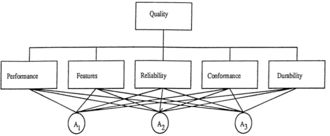
3.8 Quality attributes and alternatives le v e l... 25
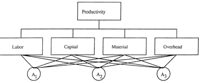
3.9 Productivity attributes and alternatives l e v e l ... 29
4.1 Ciish flow diagram of Alternative 1 ... 43
4.2 Cash flow diagram of Alternative 2 ... 43
4.3 Cash flow diagram of Alternative 3 ... 43
A .l Layout of Flexible Manufacturing Cell 50 A .2 Layout of semi-flexible c e l l ... 52
List of Tables
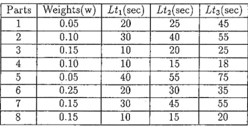
4.1 Weights and unit cell lead times of the p a r t s ... 34
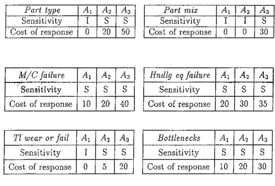
4.2 Weights and unit cumulative manufacturing lead times of the products 34 4.3 Sensitivities and cost of response'’s of alternatives to the short term changes 35 4.4 Sensitivities and cost o f response’s of alternatives to the medium term changes 35 4.5 Sensitivities and cost of response’s of alternatives to the long term changes ... 36
4.6 Annual operating costs of each alternative departm en ts... 36
4.7 Investment costs of each alternative cell during the planning horizon . 36 4.8 Market values of each alternative cell at the end of the planning horizon 37 4.9 Major level comparison m a trix ...38
4.10 Average cell lead times of the alternative s y s t e m s ... 38
4.11 Average cumulative manufacturing lead times of the alternative systems 39 4.12 Cell lead time comparison matrix of alternatives...39
4.13 Labor productivities of Ccich alternative... 40
4.14 Capital productivities of each altern ative... 40
4.15 Material productivities of each a lte r n a tiv e ... 41
4.16 Overhead productivities of each alternative... 41
4.17 Final priorities of each alternative... 44
LIST OF ТА ULFS хи
4.18 Mcijor level comparison matrix for sensitivity to cosi-first degree . . . 45
4.19 Final priorities of each alternative for sensitivity to cosi-first degree . 45 4.20 Major level comparison matrix for sensitivitj' to cosi-second degree . 45 4.21 Final priorities of each alternative for sensitivity to cosi-second degree 46 4.22 Major level comparison matrix for sensitivity to (/azns-first degree . . 46
4.23 Final priorities of each alternative for sensitivity to <
7ains-first degree
46 4.24 Major level comparison matrix for sensitivity to gains-secoud degree . 47 4.25 Final priorities of each alternative for sensitivity to ^afns-second degree 47 B .l Comparison matrix of major level a ttr ib u te s ... 55B.2 Cost comparison matrix of altern a tives... 56
B.3 Comparison matri.x of flexibility a t tr ib u te s ... 56
B.4 Comparison mati’ix of short term flexibility c h a n g e s ... 56
B.5 Part type and ¡)art mix comparison matrices of alternatives... 57
B.6 М/С failure cind handling equipment failure comparison matrices of a lte rn a tiv e s...57
B.7 Tool wear or failure and bottlenecks comparison mcitrices of alternatives 57 B.8 Comparison matrix of medium term flexibility changes...58
B.9 Demand and equipment breakdoxon comparison matrices of alternatives 58 B.IO Comparison matrix of long term flexibility changes... 58
B .l 1 New products and new raw matex'ials comparison matrices of alternatives 58 B.12 Comparison matrix of gains attributes 59 B.13 Comparison matrix of lead time a t tr ib u te s ... 59
B.14 Cell lead time and cumulative manufacturing lead time comparison matrices of alternatives... 59
B.15 Comparison matrix of quality attributes... ...60
LIST OF TABLES Xlll
B.17 Reliability and conformance comparison mati'ices of alternatives 60
B.18 Durability comp&Tison matrix of a ltern a tives... 61
B.19 Comparison matrix of productivity citirihutes... 61
B.20 Labor productivity and capital productivity comparison matrices of al ternatives ... 61
B.21 Material productivity and overhead productivity comparison matrices of alternatives...62
B.22 Quality of working life comparison matrix of a ltern a tiv es... 62
B.23 Technological improvement comparison matrix of alternatives... 62
Chapter 1
INTRODUCTION
Advanced manufacturing s}'^stems refers to Computer Integrated Manufacturing (CIM) systems and its special form Flexible Manufacturing Systems (FMS). CIM can be dciined evs “ the interaction between ]:>eople and machines with computer and information technology to integrate and automatically execute functionally related development and manufacturing tasks” [22]. FMS can be defined as “an opera tions network that combines numerically controlled equipment, automated material handling, and computer software and hardware to create an integrated system for automatic processing across work stations” [6]. These systems have many strate gic (competitive) advantages. On the other hand, they require high initial capital investment. Therefore, justification of them is very important problem for firms.
In this thesis, consideration is given to the justification of advanced manufac turing systems. Although the constructed model is general and can be applied to any kind of advanced manufacturing system justification problem, the main focus is a cell replacement (justification) problem in a cellular manufacturing system.
The model is constructed as an ai^plication of Saat5'^’s Analytic Hierarchy Pro cess (AHP) [25], [26]. The reason for using AHP is that it is difficult to measure many strategic benefits (flexibility, ciuality etc.) which are the important factors in the decision and AHP provides the ability for indirect measurement (by pairwise comparisons) on a common scale of both quantitative and subjective attributes. Thus it provides a method for combining many dimensions in a structured way.
The major strategies (the first level of the hierarchy) consist of cost, flexibility and gains. Cost is the Net Present Value (NPV) of operating and investment costs. Flexibility is the ability of the firm to cope with changes. Gains are the benefits which may result from advanced manufacturing systems other than the flexibility
CHAPTER 1. INTRODUCTION
and ^ ost related benefits.
If there i.s no mecvsure at a level except bottom (alternatives) level, benefits of each attribute at that level are provided to help decision makers make pairwise comparisons between the attributes in that level with respect to the attribute of the next higher level. If there is no measure at the alternatives level, related system parameters of each alternative to the attribute in the next higher level are provided to help decision makers make pairwise comparisons between the alternative systems with respect to that attribute.
A group of decision makers is proposed instead of a single decision maker. This group should consist of members from each level of the organization. For the pairwise comparisons, the group discusses the benefits or system parameters (alternatives level) and reaches to a consensus decision. The effects of individuals on these decisions depend on the level of the hierarchy. For example, a shop floor supervisor may be effective for the pairwise comparisons at the alternatives level, on the other hand general manager of the firm may be effective for the pairwise comparisons at the major level of the hierarchy.
This thesis consists of five chapters and two appendices. The next chapter includes the literature review. In chapter 3, the suggested AHP justification model is constructed. In chapter 4, an application of the model into a cell replacement problem in a cellular manufacturing system is provided. The last chapter presents conclusions and suggestions for further research. Appendix A includes the layouts and tli(' pro[)crti<'s of the <i.ltcm<i.liv<; systcm,s ;uid appendix II iiidude.s coiuparisou matrices, priority vectors and Expert Choice (the AHP software used) output for the application (cell replacement) problem.
Chapter 2
LITERATURE REVIEW
Justification of advanced manufacturing s3'^sterns has been a problem since the intro duction of these systems. Approaches can be categorized into two groups, namely traditional engineering economic models and multi-attribute decision models. In the literature, there are large number of papers which criticizes the deficiencies of traditional engineering economic models [3], [10], [19], [21], [24], [34] and [20]. The main points of these criticisms can be categorized as follows:
- Onl}^ short term effects are taken into account.
- Some of the benefits (especially the strategic ones) cannot be appropriately included in the evaluations because of the difficulty in quantifying many important factors.
Although many papers has been published on the deficiency of the financial measures and the need for the addition of some strategic attributes, only small number of papers which actually present a multi-attribute approach to justification have been written.
These approaches can basically be categorized into two groups; 1) Multi- Attribute Decision (Utility) Theory (M AU T) which calculates the expected utility of each alternative and selects the one with the maximum of this value, and 2) the Analytic Hierarchy Process (A liP ) which is basically designed to set priorities (by use of pairwise comparisons) for the elements in each level of the hierarchy (obtained by decomposing a complex decision problem into some levels of detail) according to their impact on the criteria or objectives of the next higher level. There are some differences between these two approaches. Firstly, M AUT is a normative pro cess, on the other hand, AHP is a descriptive theory which encompasses procedures leading to outcomes as would be ranked by a normative theory. Secondly, M AUT
CHAPTER 2. LITERATURE REVIEW
uses interval scale, however, AHP uses ratio scale. Thirdly, M AUT includes risk attitude of decision makers in the analysis. And lastl}'^, AHP has a particular way of dealing with inconsistency in judgments. Moi'eover, there are some approaches which slightly differ from these two approaches. The equivalence of most of these approaches is discussed in Falkner [14].
Sullivan [31] presents a multi-attribute decision model for making a decision between a manual or a robotic system. Draper Labs [12], Sloggy [27], Canada [7], and I'alkner and Benhajla [13] all develop multi-attribute decision models for justif3’ ing a Flexible Mivnufa.cturing Syslem.
Saatj^’s Aucil3'tic Hierarchy Process [25], [26] is applied to the justification of an FMS in Arbel and Seidman [1], Varney, Sullivan, and Cochran [32], and Srini- vasan and Millen [30] papers. Arbel and Seidman propose a performance evaluation methodology for selecting flexible manufacturing systems (FMS). In this paper, a multitude of issues relevant to the decision problem are addressed by the perfor mance evaluation framework, treating both tangible and intangible decision factors. They also present a description of one out of several real industrial application of the model. Varney, Sullivan, and Cochran discusses and applies AHP to flexible man ufacturing system justification. In this paper, it is demonstrated that important intangible benefits and costs associated with a FMS justification can be explicitly incorporated into the analysis. Both ol these papers develop separcite hierarchies for benefits and for costs. Then the priority vectors obtained from each hierarchy are used to calculate a benefit-cost ratio for each alternative as the basis for making the final decision. However, benefit-cost ratio obtained in this way has been shown to possibly result in an incorrect decision. Bernhard and Canada [2] argue the benefit-cost ratio procedure recommended by Saaty for Analytic Hierarchy Process applications having benefit and cost output vectors. In this paper, they show that this procedure does not, in general, yield an optimal solution even when benefits and costs are known with certainty and measured in dollars.
Srinivasan and Millen suggest a framework which is based on integrating a multi-attribute decision model (АИР) for evaluating qualitative data with cash flows. This is a two stage approach which considers only a hierarchy of strategic benefits and then uses the priority vector of this hierarchy to perform net present value calculations. On the other hand, in the justification model proposed in this research, cost is considered as a major attribute as well as flexibility and gains in a single hierarchy. The priority vector obtained from this hierarchy is used for the final decision.
Determination of a meaningful attribute set to use in the justification of ad vanced rncunifcicturing systems by multi-attribute decision models is an important
CHAPTER 2. LITERATURE REVIEW
problem. For example, manufacturing flexibility is a relatively new concept and be coming increasingly important Cook [11], Buzacott [5], Gustavsson [17] and others. Moreover, this concept itself is multidimensional Browne [4], Carter [8], Falkner and Benhajla [13].
There are other important factors. For instance, product quality which is again a multidimensional factor. Garvin [15] decomposes product quality into eight critical dimensions, each of which may have sets of attributes. Monetary, productivity, lead time are among the rest of the critical factors. Falkner and Benhajla [13] suggests nine major classes of potential attributes.
In the proposed justification model, some of these factors and some additional ones (quality of working life and technological iinprovemeiit) are structured into the hierarchy as major attributes. These are cost, flexibility and gains (lead time, qualit}'·, productivity, quality of working life, technological improvement).
In most of the models, Arbel-Seidman, Varne3'^-Sullivan-Cochran, Falkner and Benhajla [13], flexibility is considered among the major level attributes. Also in the proposed justification model, flexibility is considered as one of the major level attributes.
Chapter 3
JUSTIFICATION MODEL
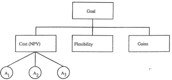
First level of the model is the “strategies” level. It consists of cost, flexibility and gains. For the pairwise comparisons at this level, the decision makers should con sider the strategic objectives of the firm and decide on the relative benefits of the attributes to those objectives via the goal. Then, they should make the pairwise com pari.sons.
Figure 3.1: Major level attributes
In the figure above, A i,A
2
, and A3
refer to the alternatives which are to be compared. They form the alternatives level (bottom level) of the hierarchy.CHAPTER 3. JUSTIFICATION MODEL
3.1
Cost (Net Present Value-NPV)
The costs of the firm affect the unit iDrices of the products, as a result profitability.
(lonscMpHiritly, iiicr<ia.s('d proiit<i.l)iIity improves tlic market sliare and compt'titiviiiiess
of the firm
Cost elements that should be considered in the analysis of advanced manufac turing systems and their estimates are provided to be able to generate cash flows over a project life. Fourteen cost elements are defined for each period during a planning horizon.
Project life is assumed to be composed of a planning horizon (N ) on which cost calculations are based. Total costs in each period of the planning horizon is considered as the cash flows over the project life. The Net Present Value (NPV) is calculated for each of the alternative manufacturing systems.
Guidelines for the decision makers to make the pairwise comparisons between the alternative systems are as follows. First, they should consider the NPV of each alternative system. Then, they should decide on the lowest (possible) value and the highest value for NPV. Finally, the}^ should make the pairwise comparisons.
Since the alternative systems other than the existing system are not opera tional, computer simulation of the manufacturing system may be used as a tool for the collection of cost related datii.
Because of the thorough treatment of cost in Son and Park [29] and refined in Son [28], the following notation and description are for the most part taken directly from these papers. In both papers, opportunity costs are included to represent the consideration of flexibility issues. Flexibility is treated differently in this model and discussed later.
3.1.1
Investment (replacement) cost
The investment cost for an alternative system is the cost of replacing the whole (or a part of, e.g., old machines) manufacturing system and making it operational. It
be calculated as
A"3
where:
INVt = investment cost of the manufacturing system at year t, L {k,t) = number of manufacturing equipment k replaced at year t,
= cost of acquiring a unit of mamil'acturing ccpiipinciit k, Cn{k) = cost of installing a unit of manufacturing equipment k,
Co{t) = cost of preparing (integrating, testing, etc.) the system for the regular production at year
Cp{t) = opportunity cost of lost productive value during the replacement peri od at year t,
Cr = current (year 0) market value of the system. It is zero for the alterna tive systems other than the existing one,
KS = total number of pieces of manufacturing equipment.
3.1.2
Labor cost
Labor cost is the cost of direct and indirect labor. It includes wages, salaries, and fringes benefits. It may be defined as
CHAPTER 3. JUSTIFICATION MODEL 8
Ll L2
C'l = ^ CdTld + ^ CiUi + Cfr
d=l 1=1
where:
Cl = labor cost during a 3^’ear,
In = number of different jobs using direct labor,
¿ 2
= number of different jobs using indirect labor,Cd = wage of job d in a year,
Ci = salary of job i in a year,
Cfr = fringes for direct and indirect labor in a year,
Ud — number of direct labor units for job d,
Ui = number of indirect labor units for job i
3.1.3
Material cost
Material cost consists of all the costs related with the preparation (ordering, pur chase, and transportation) of materials (direct and indii'ect) for the production. It ma.j'· be defined as
CHAPTER 3. JUSTIFICATION MODEL
c'H = X ; a / ( i ) n j ( i ) + c ',, + a J=1
where;
Cr = material cost during a year,
Co = total material ordering cost per year, J = number of different parts,
Cd{j) — unit cost of direct material for part j,
f^d{j) — amount of direct materials used for pa-rt j per j^ear,
Cid = indirect material cost except tools per year.
3.1.4 Machine cost
Machine cost consists of utility, maintenance, repair, insurance, and property tax costs for manufacturing equipment. It may be defined as
K3
Cm — + Cr{k)Tr{k) + ah\ + bE\^
k=l
where:
Cm = machine cost during a year,
Cu{k) = utility cost of machine k per unit time,
Cmt{k) = maintenance cost (including lost productive value) of machine k per unit time,
Cr{k) = repair cost (including lost productive value) of machine k per unit time,
Tm{k) = total machine time of machine k per year,
Trnt(k) = total maintenance time of machine k per
5^ear,
Tr{k) = total repair time of machine k per year,
a = insurance premium rate,
b = property tax rate,
Fk = first cost (initial investment) for machine k.
3.1.5
Depreciation cost (inflow)
Depreciation cost refers to the recovery cost of manufacturing equipment and facil ities. It is the only element which is inflow to the cash flow analysis. It may be
CHAPTERS. JUSTIFICATION MODEL 10 defined as Kl D C = rr Cd{k) ¿=1 where;
D C = depreciation cost during a year,
rx — tax rate,
Cd{k) — annual depreciation cost of asset k,
Jv4 = number of assets.
3.1.6
Tool cost
Tool cost consists of cost of maintenance (labor cost) for the cutting tools and costs of cutting tools in case of replacement due to wear and breakage. Using the regular tool changes principle (i.e. assuming a useful tool life and regularl}^ changing a tool before it reaches its average tool life), tool cost may be defined as
M
C't = ^ cti{m){n^{m) + nb(m)}
m=l
where:
Ct = tool cost during a year,
Cti{m) = unit cost of tool type m,
n^(m) = number of worn tools of type m per year,
ni)(m) = number of broken tools of type m per year, M = number of different tools.
3.1.7
Floor space cost
Floor space cost consists of utilities, maintenance, repair, insurance, and property tax costs of manufacturing floor space. It may be defined as
Cs = CspSm
where:
Cs = floor space cost during a year,
Csp = space cost per square foot per year,
CHAPTER 3. JUSTIFICATION MODEL 11
3.1.8
Computer software cost
Compviter software cost is the cost associated with maintaining computer softwares. For a planning horizon, it may be defined as
s
Csw — ^ ^
s=l
where:
Csw — computer software cost during a year,
Cms{s) = membership fee of software type s per year,
Tisyj(s) = number of software type s,
S = number of different software programs.
3.1.9
Prevention cost
Prevention cost refers to the cost of inspecting and correcting in-process quality problems before final inspection. It consists of appraisal and prevention costs. It may be defined as
J K1
j=l k=l
where:
Cp — prevention cost during a year,
Cp{j, k) = prevention cost of part j for machine k per year (see Son [28] for a de tailed calculation procedure),
K1 = number of machines except material handling systems and computers.
3.1.10
Failure Cost
Failure cost refers to the cost of loss that results from failure of finished products to satisfy quality standards set by both the firm and customers. It consists of internal and external failure costs. It may be defined as
Cf =
CHAPTER 3. JUSTIFICATION MODEL 12
where:
Cp = failure cost during a year,
Cf(j) = failure cost of part
Qj — amount of part j produced per year,
+ fi'’[p]{(l - ei - C2)ct + (1 - e2)(l - w)Cs + tiC a }
(assuming Cg — Cb)
where:
Cg — cost of reworking a good part because of misclassification,
Cb = cost of reworking a bad (defective) part,
Cs = cost of scrapping a defective part that could not be restored,
Ca = cost of accepting a defective part,
p = proportion defective of a part.
Cl = error rate of misclassifying a good part into defective (type I error), C
2
= error rate of misclassifjdng a defective part into good (type II error),■w = rate of restoring a defect to a good part.
3.1.11
Setup Cost
Setup cost refers to the preparation cost of machines for the production runs. It may be defined as
K2
A = Y^C,u{h) k=l
where:
A = setup cost during a year,
Csu{k) = setup cost for machine k per year,
K2 = number of machiires excluding computers.
Relations between the K 1,K 2^K 3,K 4l values can be summarized as follows: /\3 = /ti4—(number of buildings)
/v2 = Jv3—(number of computers )= /0 + (n u m b e r of material hcindling sys tems).
e n A PTER 3. JUSTWJCATION MODEL 13
3.1.12
Idle Cost
Idle cost is the opportunity cost of lost avciilable time of mcinufacturing equipment. It may be defined as
K2
Cl = i/e(A;)(l - Uk)
k=l
where:
(7/ = idle cost during a year,
Uk = utilization of ma.chine k,
Ue{k) = opportunity cost (idle cost) of machine k per year.
3.1.13
Waiting Cost
Waiting cost is the cost associated with the work-in-process inventory (W IP). It may be defined as J -P>+i J Cw = ~ 1) — Pj -H l)n (j, Pj -f 1)] j=l p=0 j=l where: C w = P,· = TUJ,p) n {j,p) {n {j.p -
1
) - n {j,p )} n ■)waiting cost during a year, number of processes for part y,
cumulative waiting time of part j up to process p, number of raw materials for part j that have entered the manufacturing area per yca.r=l''Kj,
number of part j that completed process p per year, amount of WIP (end of year) between processes p-1 and p,
{j, Pj
1
) = total number of finished parts j per yea,v—Qj,opportunity cost (waiting cost) per unit time.
k'u, =
3.1.14
Inventory cost
Inventory cost refers to the costs related with inventory existence and stockouts. In tills element, consideration of inventory is in terms of raw material and finished
CHAPTER 3. JUSTIFICATION MODEL 14
products (VVIP inventory is considered in waiting cost element). It may be defined as
C,J = CspSt + ^ ?7ra.T[0, (c,.m (j){7o„,(i) + Uj - Wj] + Csj{j){Ios + Qj - ^ i ) ) ]
j=i
J
+ ^
max[0, {cbm{j){Wj - Uj - Iom{j)]+
Cbj{j){Dj - Qj - Ioj{j)])]where: Ch Cjp Si U: D , Iorn{j) ^sm { j ) ^bm (J ) C 6 / ( i ) J = 1
= inventoiy cost during a year,
= space cost per square foot per year, = warehouse space,
= amount of raw materials obtained from suppliers per year, = demand rate for part j per year,
= initial inventory of raw materials for part j,
= initial inventory of finished part j,
= cost of Ccinying a unit of raw material of part j per year, = cost of carrying a unit of product of part j per year, = shortage cost of a unit of raw material of part j per year, = shortage cost of a unit of finished product of pcirt j per year.
3.2
Flexibility
In the context of manufacturing systems, flexibility can be defined as the “ ability to cope with changes” (Mandelbaum [23]). The benefit from flexibility is the enhance ment of the firm’s ability to better cope with uncertaint}'·. This results in the ability to respond to customer needs ahead of competition consistently and predictably and to respond rapidly to nuirket change with respect to: product mix, product volume and product change.
To evaluate the flexibility of the alternative manufacturing systems, the nature of the changes and disturbances with which the systems should be able to cope must be considered. Tliese changes become the biisis for tlie evaluation of the cdteriiative manufacturing systems.
In this research, time scale decomposition was chosen to be utilized for struc turing changes. In the manufacturing literature, Gustav.sson [17] appears to be the first to recognize the importance of time scales to the understanding of flexibility.
CHA PTER 3. JUSTIFICATION MODEL 15
Recently, Carter [8] argued that “different types of flexibility irnpa.ct production in different time frames” . However, Gupta and Buzacott [16] argue that a variation of the above principle where changes not types of flexibility are categorized according to time frames has the advantage that changes which take effect over different time scales often differ in their scope as well. For instance, short term changes affect the cells, medium term changes affect the department and long term changes affect the firm.
Simplifying assumptions of the time scale decomposition which is proposed by Gupta and Buzacott [16] can be provided as follows:
1. All state variables at time scales higher than that of the current subproblem may be assumed to be constant.
2. All changes in state variables at time scales lower thiin that of the current subproblem may be aggregated.
These assumptions are considered by decision makers while making the pair wise comparisons related with flexibility attributes. For example, while considering a short term change (e.g., calculating the “cost of response” terms for each alterna tive system), decision makers may assume the state variables at medium and long term time frames as constant. And, while considering a long term change, decision makers may aggregate all changes in state variables at short and medium term time frames.
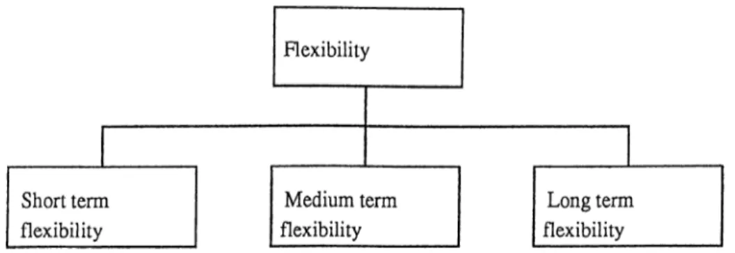
Figure 3.2: Flexibility attributes
B}'^ using decomposition of changes according to time scales, three categories of changes may be identified, namely, short term, medium term and long term changes. Ability to cope with these categories of changes will determine the short term, medium term and long term flexibilities which are the attributes of “flexibility” . For making the pairwise comparisons among these attributes, guidelines for the decision makers are as follows. First of all, they should consider the benefits of each attribute to “flexibility” by considering the benefit information provided under each one. Secondly, they should think of loosing a “specified level” (e.g., a specified
CHAPTER 3. J USTIFICATION MODEL 16
percent) of one of these attributes for a fixed period of time. After passing the above two steps for each attribute, they should judge the relative importances (opportunity losts in the second step) of these attributes to the “flexibilit}'^” . Finally, they should make the pairwise comparisons.
Similar guidelines are followed for the pairwise comparisons among the at tributes of short, medium and long term flexibilities.
3,2.1
Short Term Flexibility
Short Term Flexibility (STF) is the abilit}^ to cope with short term changes. Short term changes may be cifectivc for a period of a few minutes to a few hours, individu ally, each short term change affects the system less significantly (only the individual cells) than medium or long term clmnges. On the other hand, short term changes occur very frequently and their collective action may result in significant production losses if the system does not respond effectively. Therefore, benefit of coping with these changes is to protect the cells from production losses.
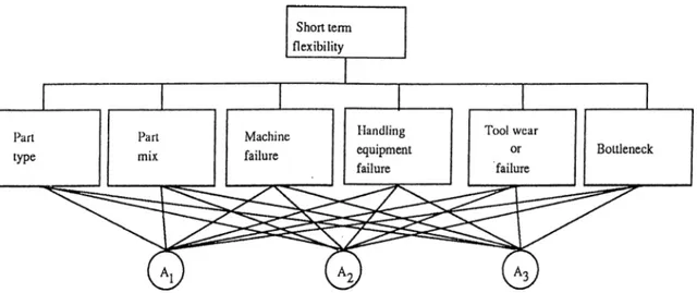
STF can be separated into six attributes (changes), namely, “part type” , “part m ix” , “machine failure” , “handling equipment failure” , “tool wear or failure” , and “bottlenecks” .
Figure 3.3; Short term flexibility attributes and alternatives level
As it is mentioned earlier, flexibility definition includes the term ^^abiliti/\ For the alternatives level pairwise comparisons, this term will be separated into “sensi tivity” and “stability” terms. As described in Gupta and Buzacott [16] “sensitivity” relates to the degree of change tolerated before a deterioration in performance takes
CHAPTER 3. JUSTIFICATION MODEL 17
place. If a S
3^stem is sensitive to a change, then its “stability” relates to the mag
nitude of each disturbance for which it can meet performance levels expected of it in a reasonable time. In other words, while sensitivity determines whether or not a response is needed, stability determines whether or not a system is capable of responding given that a response is needed.Pairwise comparisons in the alternatives level will depend on the “cost of re sponse” values of the changes which have the following equation:
= P{ uj ) + i — 1, , m j = l ,. ., n
where:
c{i,j) = estimated cost of response of alternative i to change j,
p { i j ) = estimated cost of production loss of alternative i during the time of response to change j,
r( i , j ) = estimated expenses (other than production loss) for the response of alternative i to change j,
m = number of alternative systems,
n = total number of changes.
Simulation can be used as a tool for the determination of estimated costs in the above equation.
Following this definition, each of the attributes (changes) of STF will be con sidered in detail as follows:
“Part tj'pe” is related with the change in the type of part being produced at a machine that requires no new setup of the tool magazine, jigs and fixtures. This change may affect the processing times of the parts (as a result, it may cause to the bottleneck of the machine), therefore rescheduling of machines in the cell level may be required to cope with this change. Coping with this change brings the benefit of protecting productivities and production rates of the cells.
Related system parameters are capabilities of machines (e.g., average number of processes that the machines can perform) and degree of integration of the system to provide easy scheduling. For making the pairwise comparisons at the alternatives level of this change (attribute), guidelines for the decision makers are as follows. First of all, decision makers should consider the related system parameters to realize the capabilities of the alternative systems in terms of the change. Secondly, they should judge (subjectively) the sensitivity of each alternative system (i.e. alternative cell, since the change affects the cells individually, there is no difference between the
Cl IA PTFAl 3. .WSriFICATION MODFI. 18
alternatives in terms of the cells other than the cell under consideration. Therefore, it is cnougli to compare the alternative codls at tliis level ). The sy.stcm which is insensitive to the change hcis zero “cost of response” . If a system is sensitive to the change, then decision makers should consider the stability of that system. If it is unstable (i.e. incapable of coping with the change in a reasonable time), then it is assigned very high (e.g., M) “cost of response” value. Otherwise, its cost of response is calculated. After having the “cost of responses” calculated for each alternative system, decision makers should decide on the lowest (possible) and highest value of “cost of response” for the change. As the final step, they should make the pairwise comparisons.
Similar guidelines are followed for all the pairwise comparisons at the alterna tives level of flexibilities (short, medium,long). However, in medium and long term changes, alternative systems refers to alternative departments (since the medium term changes affect the department) which are the departments including alterna tive cells and alternative firms (since the long term changes affect the firm) which are the firms including alternative cells, respectively.
“Part mix” is related with the changes in part mix at a machine. These changes may result in the new setup of the tool magazine, jigs and fixtures. It may affect the processing and setup times of the machine, as a result rescheduling of machines at the cell level may be required to cope with this change. Coping with this change brings the benefit of easier routing of the parts in the cells.
Related system parameters are the capabilities of machines (average number of operations that the machines can perform, average setup (time) requirements between the operations etc.).
“Machine failure” is the third change (attribute) of STF. Changing the routings of the parts to the alternative machines (as a result rescheduling of the alternative machines and the material handling equipment) may be required to cope with this change. Coping with this change brings the benefit of protecting the production rates of the parts processed on the machine.
Related system parameters are average number of processes that the machines can perform and ease of scheduling of machines and material handling equipment.
“Handling equipment failure” is the fourth change (attribute) of STF. During the repair time, allocation of new material handling equipment or rescheduling of other existing handling equipment may be required to cope with this change. Coping with this change brings the benefit of protecting the production rate of the cell which has handling equipment failure.
CHAPTER 3. JUSTIFICATION MODEL 19
Related system lijarameters are the average number of material handling equip ment in the cells, their ease of scheduling and opportunity of alternative handling eciuipment.
“Tool wear or failure” is the fifth change (attribute) of STF. During the re placement time, changing the routings of the parts related to the machine which needs its tools to be replaced (as a result rescheduling of the alternative machines and the material handling equipment) may be required to cope with this change. Coping with this change brings the benefit of protecting the production rates of the parts related with the machine which has tool wear or failure.
Related system parameters are average number of processes that the machines can perform and ease of scheduling of machines and material handling equipment.
“Bottlenecks” results when there becomes a contention among the common users of a resource (e.g., for raw materials, pallets, machines, material handling equipment, and tools). Alternative resources for the common users (e.g., alternative machines is a solution for the bottleneck of a machine) may be required to cope with this change. Coping with this change brings the benefit of productivity improvement in the cells.
The following ¡procedure is used to determine the “cost of response” terms of the alternative systems for the “bottlenecks” . First, for each alternative system, “cost of response” for the bottleneck of each resource (e.g., raw materials, pallets, machines etc.) is determined by assuming each of these bottlenecks as single changes. Secondly, average of these “cost of response” terms is obtained for each alternative system. Finally, these averages are considered as the “cost of response” terms of the alternative systems for the “bottlenecks” .
Related system parameters are the parameters (e.g., average number of pro cesses that the machines can perform) that determines the capabilities of the alter native systems (ease of systems) in providing alternative resources.
3.2.2
Medium Term Flexibility
Medium Term Flexibility (M TF) is the ability to cope with medium term changes. Changes belonging to this category may have a time scale ranging from a few days to a few months. These changes are mostly department related changes, i.e. each one affects the department as a whole. They can be coped with by the integrated efforts of the department resources. Individually, each medium terra change occurs less frequently, but may affect the system more significantly than short term changes.
CHAPTER 3. JUSTIFICATION MODEL 20
Benefits oi coping with these changes are to protect the production rate of the department and respond to the medium term market fluctuations.
MTF can be separated into two atti-il)utes (cliariges), namely, “demand” and “equipment breakdown” .
Figure 3.4: Medium term flexibility attributes and alternatives level
Each one of these attributes will be considered in detail as follows:
“Demand” is related with the change (increase) in the demand for certain products (as a result, parts related with the department) where the production capacity and the long term average demand do not change. Such changes may be caused by lorccast errors or by market lluctuations. Increasing the production rates of the cells (critical cells) which are related to the products may be required. This mciy be accomplished by allocating noncritical parts to the noncritical (other less utilized) cells to increase the availability of the critical cells for the products under consideration. The benefits of coping with this change are to protect the firm from profit loss aird customer goodwill loss.
Related system parameters are the utilizations of the resources in the cells, and ease of allocating parts from one cell to another (depends on the parameters like number of processes that the machines can perform, ease of scheduling the machines and material handling equipment etc.).
“Equipment breakdown” is related with major machine or handling equipment breakdowns (e.g., major machine may be a heat treatment msichine and major handling equipment may be an intercellular material handling equipment). During the breakdown period, allocation of alternative equipment may be required to cope with this change. The benefit of coping with this change is to protect the production
CHAPTER 3. JUSTIFICATION MODEL 21
oi the depcirtineiit and as a result the production of all products dependent on the department. At the end, the firm is protected from profit loss and customer goodwill loss.
The related system parameter is the availability of alternative major equipment resources in the department.
3.2.3
Long Term Flexibility
Long Term Flexibility (LTF) is the ability to cope with long term changes. Long term changes occur infrequently. However, they have very significant effects and may be effective over a period ranging from a few months to a few years. These changes affect the firm. They can be coped with by the efforts of all the departments and the firm. The benefit of coping with these changes is to increase the competitive power of the firm.
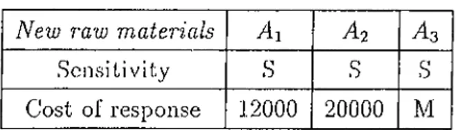
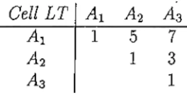
LTF can be separated into two attributes (changes), namely, “new products” and “new raw’ materials” .
Long-term flexibility
New New raw
products materials'
Figure 3.5: Long term flexibility attributes and alternatives level
Each one of these attributes will be considered in detail as follows:
First one is introduction of “new products” (as a result, introduction of new parts to the department). Allocation of parts (related to the department) of new products to the cells or new part-family formation may be required to cope wdth this change. The benefit of coping with this change is to respond to the market changes (competitive advantage).
CHAPTER 3. JUSTIFICATION MODEL 22
Related system parameters are utilizations of the cells, capacity of the cells and average number of processes that can be performed in the cells.
Second attribute (change) is the development of “new raw materials” . Re designing the products with regard to new raw materials and allocating the depart ment related parts to the cells (or new part-family formation) maj^ be requii'ed to cope with this change.
The benefits of coping with this change are opportunities of product quality increases and cost reductions which result in competitive advantage.
Related S
5'stem parameters and guidelines for the decision makers to make the
pairwise comparisons at the alternatives level of the change are the same as that of “new products” .3.3
Gains
These are the benefits (that may be gained from the advanced manufcicturing sys tems) other than the benefits related with “flexibility” and “cost” (NPV). They improve the profitability, market share and competitiveness of the firm.
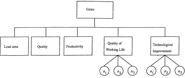
Figure 3.6: Gains attributes
“ Gains” attribute can be separated into five attributes, namely lead time, productivity, quality of working life, and technology. For making the pairwise com parisons among these attributes, guidelines for the decision makers arc as follows. First of till, they must consider the benefits of each attribute to “gains” by consid ering the benefit information provided under each one. Secondly, they should think
CHA PI.'ER 3. J USTIFICATION MODEL 23
oi losing a “specified level” (e.g a specified percent) of one of these attributes. After passing the above two steps for each attribute, they should think of the relative im portances (opportunity losts in the second step) of these attidbutes to the “gains” . Finally, they should make the pairwise comparisons.
3.3.1
Lead Time
Jotii.1 lead time is tlie time which ehipses between the moment an item is ordei’ed (make-to-order or make-to-stock) and the time it is available for use. Lead time has the following elements:
Lead time = generating paperwork -f purchasing -f- setting-up -1- waiting
+ queuing -1- processing + movement
“Generating papei'work” includes determining requirements, linking into the control systems and ordering; “purchasing” is the time it takes for an item to be delivered from a supplier; “setting-up” is the time involved in setting up the set of processes for completing the particular operation(s); “processing” is the actual time that the job is being worked on; “movement” is the time that a job spends in transit from one process to the next; “waiting” is the time that a job waits before being moved to the next process; “queuing” is the time that a job is waiting to be worked on because another job is already being worked on in that process [18]. Since the first two of these elements have the same values in all of the alternative systems, they do not affect the judgments in the pairwise comparisons. Therefore, lead time will be considered in terms of the last five elements.
Under this attribute, we will consider “intangible” benefits from improved lead time. First one is related with quality. Quality is enhanced by the rapid identification and correction of problems before too many defective subassemblies and/or finished products are built. Low lead time result in rapid detection and correction of quality problems.
Second one is the reduction in the response time to the market. With a short lea.d time, it is easier to respond to changes in the market.
Lastly, a set of benefits results through the shortening of planning horizon. First of all with a shorter phinning horizon, there can be less reliance on forecasts and more on confirmed customer orders. Thus, a company can approach being a make-to-order company if it previously is a made-to-stock. Second, by forecasting over a shorter horizon, the accuracy of the forecast is likely to improve. This will lead to better balanced and lower inventories (tlie quantitative benefits of this inventory
CHAPTER 3. JUSTIFICATION MODEL 24
reduction and balance are included in the cost attribute). Further, shorter planning horizons with more reliance on accepted customer orders and better forecast accu racy can improve the stability in manufacturing schedules (a highly desirable feature in Production Planning and Control systems). This results in fewer opportunities for scheduling of open orders and therefore, creates a less “nervous” sj'^stem [33].
Since two of the alternative systems (except the existing one) are not op erational, simulation can be used for the estimation of lead times (both cell and cumulative manufacturing) of each system. An easier method would be to sum the estimated values (if such estimates arc available) of the five elements mentioned above.
Lecid time can be separated into two attributes, namely cell lead time and cumulative manufacturing lead time. The cumulative manufacturing lead time can be reduced if parts produced in the cell being considered are “bottlenecks” with respect to end product delivery. If this is not the case, onl}'^ local benefits (like rapid detection cind correction of cell quality problems) will be achieved from cell lead time reduction.
Figure 3.7: Lead time attributes and alternatives level
For making the pairwise comparisons among these attributes, guidelines for the decision makers are as follows. Firstly, they should consider the benefit that results from cell lead time reduction. This is the first benefit mentioned above which affects only the cell. Secondly, they should consider the benefits that result from the cumulative manufacturing lead time reduction. These are all of the benefits mentioned above. Thirdl)q they should think of losing a “specified level” of one of these attributes. After passing the above steps for each attribute, they should think of the relative importances (opportunity losts) of these attributes to the “lead time” .
Cl I A PTER 3. J USTIFICA TION MODEL 25
Finally, they should makci the:: pairwise coinparisoiis.
Alternatives level pairwise comparisons for each attribute depend on the lead time estimates. Guidelines for the decision makers are as follows. First, they should consider the value of the related lead time estimate (cell lead time or cumulative manufacturing lead time) for each one of the alternative systems. Then, they should decide on the lowest (possible) value and the highest value of this lead time. Finally, they should make the pairwise comparisons.
3.3.2
Quality
Product cpiality is rapidly becoming an important competitive issue. David A. Garvin [15] suggests that the quality should be broken down into manageable parts to consider it as a strategy. He proposes eight critical dimensions or categories of quality that can serve as a framework lor strcitegic anaH'sis : performance, featui-es, reliability, conformance, durabilitj'^, servicability, aesthetics, and perceived quality. The first five of these critical dimensions will be considered under our quality at tribute. The others do not significantly depend on the type of alternative system; therefore, they do not affect our decision.
Figure 3.8: Quality attributes and alternatives level
Under this attribute, we will consider “intangible” benefits from improved quality. Which quality attributes are more important than the others depends on the strategy of the firm.
Improved quality provides benefits for the firm. The first one Is related to market share. The relationship between qualit)'· and market share is likely to depend
CHAPTER 3. JUSTIFICATION MODEL 26
on how quality is defined. If a high-qualit}' product is one with superior performance or a large number of features, it will generally be more expensive and will sell in smaller volumes. But if quality is defined as fitness for use, superior aesthetics, or improved conformance , it need not be accompaiiio'd liy proiniiim prices. In tha.t case, quality and market share are likely to be correlated positively.
The second benefit is related to profitabilitjc Improved quality may lead to higher profitability in two ways. The first is through the market: improvements in performance, features, or other dimensions of quality lead to increased sales and a larger market share or, alternatively, to less elastic demand and higher prices. If the cost of achieving quality gains is outweighted by the increases in the contribution to profit then the firm should undertake these gains. Qualit}' improvements may also affect profitcibility through cost. Fewer defects or field failures result in lower manufacturing and service costs. As long as these gains exceed any increase in expenditui'es by the firm on defect prevention, profitability will improve.
As it was mentioned earlier, “quality” attributes considered in our model are performance, features, reliability, conformance and durability. For making the pair wise comparisons among these attributes, guidelines for the decision makers are the same as tliat of “gains” .
Each of these attributes is discussed below:
Performance refers to the primary operating characteristics (objective charac teristics) of a product. Performance of a product provides benefits to the consumers. Therefore, if the objective characteristics of a product can better satisfy consumers, it may result in improvement in the market share of the firm.
The capabilities of machines and material handling system (primary and sec ondary) of the cell may cause a difference in the performances of the products processed by the alternative systems. They can provide capabilities to make designs which may improve the objective characteristics (as a result, perforrmmee) of tlie products. Tiierefore, these capabilities of the alternative systems are considered as the performance related S
3'’stem parameters. Guidelines for the decision makers
to make the pairwise comparisons at the alternatives level of “performance” are as follows. First of all, they should consider the related system parameters to realize the capabilities of the alternative systems in terms of the “performance” . Secondly, they should judge on the relative importances of the alternative systems in providing more design capabilities which means better objective characteristics. Finally, they should make the pairwise comparisons.CHAPTER 3. JUSTJEICATION MODEL 27
whistles” of the products; those characteristics that supplement their basic func tioning. The benefits related w’ith performance are also valid for this attribute.
Again the capabilities of machines and material handling s}^stem of the cell may allow for designs which offer more features to the consumei's. Therefore, features related system parameters and guidelines for the decision makers are the same as that of “performance” .
Reliability is the probability of product’s failure within a specified period of time. It is difficult to measure reliability quantitatively. Because all quantitative measures recjuire a product to be in use for a specified period or to be subjected to a life testing program. However, e.xcept for the existing alternative system, there is no usage or test data.
Reliability is essential for every product. It becomes more important to con sumers as downtime and maintenance become more expensive.
An automated alternative system has the advantage of less human error. Hu man errors which can not be determined by the inspection tests ma}'^ result during material handling (causing damages in the product during its transportation be tween workstations) and loading-unloading operations (causing damages because of wrong adjustments etc). As a result, the system which uses more human effort produces less reliable products.
By increasing the capabilities of machines, material handling system, inspec tion modules, degree of automation, and degree of integration of the cell; design opportunities which may offer more reliable products to the consumers are gained. Therefore, these capabilities of the alternative s3^stems are considered as the relia bility related system parameters. Guidelines for the decision makers are as follows. First of all, they should consider the related system parameters to realize tlie ca pabilities of the alternative systems in terms of the “reliability” . Secondl}', they should judge on the relative importances of the alternative systems in providing less human errors and more design capabilities which means better reliabilitje Finally, they should make the pairwise comparisons.
Conformance is the degree to which a product’s design and operating charac teristics match established standards. Benefits of having conformance to the estab lished standards are to decrease the service call intensity (because of inconformance to the standards, not because of breakdowns-unreliability) which means better cus tomer satisfaction and defect rates in the factory (included in the cost attribute).
Conformance of the system depends on the capabilities of the machines, mate rial handling systems (primary and secondary), and inspection processes of the cell.