Improving the accuracy of indoor positioning system

For this purpose, the test area has been divided into grids and an extensive process has been carried out to determine an average path loss index value based on RSSI

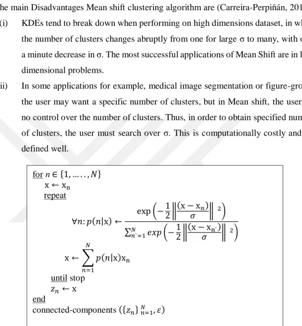
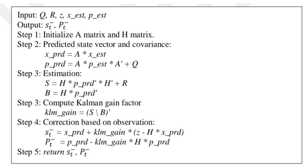
These methods are K-means, fuzzy c-means, and mean shift for clustering, the Kalman filter, and finally, the average silhouette method to initialize the optimal number of

In the study of Yang et al (8) natural killer cell cytotoxicity and the T-cell subpopulations of CD3+ CD25+ and CD3+HLA-DR+ were increased significantly after 6 months

The theory regarding mechanism of hematocrit in CHD is limited. Hematocrit, the proportion of the total blood volume occupied by red blood cells, is a major determinant

Figure 11-23a Molecular Biology of the Cell (© Garland Science 2008) K+ Kanalları: Na+ kanalları ile benzer çapta olmalarına rağmen 10.000 kat daha iyi iletir.. Tek bir amino asit

Figure 15-52 Molecular Biology of the Cell (© Garland Science 2008) 59 Reseptör Tirozin Kinazlar: En büyük ligand grubunu Efrinler oluşturur, Eph reseptörlerine bağlanırlar!.

Mix granules under 1.00 mm sieve (less than 1.00 mm) and repeat the above procedure to calculate the bulk volume (V k ), bulk density ( k ) and tapped density ( v ) HI

Each repeater used in the GPS based indoor positioning system is composed of a directional receiver antenna, an LNA block, an additional amplifier for loss