Başlık: Estimation of time varying parameters in an optimal control problemYazar(lar):ÖZBEK, Levent; KÖKSAL BABACAN, Esin Cilt: 64 Sayı: 2 Sayfa: 111-121 DOI: 10.1501/Commua1_0000000738 Yayın Tarihi: 2015 PDF

Volume 64, Number 2, Pages 111-121 (2015) DOI: 10.1501/commua1-2_0000000738 ISSN 1303-5991

Received by the Editors: September 05, 2015; Accepted: December 22, 2015.

Key words: Non-linear state space models, Extended Kalman filter, Optimal linear regulator

1_{Ozlale (2003) and Salemi (1995) are some of the exceptions in this context.}

© 2015 Ankara University ESTIMATION OF TIME VARYING PARAMETERS IN AN OPTIMAL

CONTROL PROBLEM

LEVENT ÖZBEK and ESIN KÖKSAL BABACAN

ABSTRACT. In this paper, we employ a non-linear state space model and the extended Kalman filter to simultaneously estimate the time-varying parameters in an optimal control problem, where the objective (loss) function is quadratic. Our methodology also allows us to derive the difference between the optimal control and the observed control variable. A simulation exercise based on a simple intertemporal model shows that the estimated parameter values are very close to their population values, which provide further support for the estimation methodology introduced in this paper.

1. INTRODUCTION

Although there has been an ever-growing increase in the number of studies, which utilize optimal control techniques in economics, the literature is relatively silent in the estimation of the parameters in an optimal control set-up 1 _{. In other words, given the observation, state and}

the control variables, developing estimation techniques for the parameters of a system needs to be explored in details.

Especially when the parameters in an optimal control problem are assumed to vary over time, which is a general characteristic of the models that employ large data sets, estimation of the time-varying parameters become even more important and complex.

This study tries to fulfill the above-mentioned gap in the literature by introducing an estimation algorithm for the time-varying parameters of an optimal linear regulator problem, which has a quadratic objective (loss) function and a linear system of constraints. As it will be clearer, estimating the state vector and the time-varying parameters simultaneously will cause a linearity in the system, which leads us to cast the model in a state space form and employ a non-linear filter, namely the extended Kalman filter. This algorithm is very useful method to parameter estimation in nonlinear state-space models but very small using in economic literature. In economic literature, Grillenzoni (1993), Bacchetta and Gerlac (1997), Ozbek and Ozlale (2005) used this method in their studies.

In order to test the estimation accuracy of the above mentioned method, we also conduct a simulation exercise and estimate the parameters for a simple intertemporal consumption-saving model of a representative household. The exercise shows that the estimated parameters using the non-linear state space framework and the extended Kalman filter are very close to their generated population values, supporting the estimation method introduced in this paper. The outline of the paper is as follows. First, we briefly introduce the linear and the non-linear state space models, which are frequently used in an optimal control framework. Then, we will define the optimal control problem, for which we show the estimation methodology of the parameters. The simulation exercise follows. Finally, the last section concludes the paper.

2. THE LINEAR DISCRETE-TIME STATE SPACE MODEL A linear state space model can be defined as:

1= n n n n n n n x_  x B u G w (1)

, =

n n n n n n

x

 

y H x



v

(2)

where xn nis the state vector, m n

y

 

is the observation vector and un r is the control variable vector. In addition, n and Hnshow the nn dimensional transition matrix and the mn dimensional observation matrix, respectively. Finally, wn n and

m n

v

 

represent the zero-mean white noise processes, which are the disturbance terms of the model. The assumptions about these white noise processes can be written as:

 

n

0

E v



(3)

 

n

0

E w



(4) n j n nj E v v_  _ R (5) n j n nj E w w_  _ Q (6) 0 n j E v w_  _ (7)

 

0 0 E x x (8)



( 0 0)( 0 0)



0 E x x x x  P (9)

 

0 n

0

E x w

 

(10)

 

0 n

0

E x v

 

(11)

It is further assumed that for n0,1, 2,...the matrices n,H Qn, n and Rn are known with certainty. Given these conditions and the observation vector

Y

n





y y

0

, ,...,

1

y

n



, the Kalman

filter, which is stated in Kalman (1960), emerges as a possible algorithm to estimate the state vector

x

n (see Appendix 1).

3. NON-LINEAR STATE SPACE MODELS AND THE EXTENDED KALMAN FILTER

On the other hand, a non-linear state space model can be represented as:

 

 

1

( )

n n n n n n

x





F



x



G



u



w

(12)

( )

n n n n

y



H



x



e

(13) where, F G, and H represent the vector-valued functions. In addition,

w

n and

e

n are the white noise processes with covariance matrices,

R

1

 



n and

R

2

 



n , respectively. The vector

n



represents the time varying parameter vector to be estimated. It is important to note that, the time varying parameters and the state vector is in multiplicative form, which rules out the assumption of linearity and makes it necessary to use the extended Kalman filter, as mentioned in Ljung and Söderström(1985) (see Appendix 2).

4. THE OPTIMAL CONTROL PROBLEM

Finally, the form of the dynamic quadratic loss function, for which the parameters will be estimated, can be defined as:



' ' '



0 1 1 0 =E n 2 , 0 1 N n n n n n n n J  x R x u Q u x Wu       



(14) The problem of determining the control sequence

u





u u

0

, ,...,

1

u

N1



is known as the

discounted stochastic regulator problem. In the above function, R1 and Q1 are non-negative symmetric matrices and.



is discount factor. As stated in Ljungqvist and Sargent (2000) an explicit solution of the above form is given as:

n n n

u

 

F x

(15)

 





1



 



1 ' 1 1 ' 1 1 ' n n n F  Q B P _ B  B P _  W (16)      







 





 



1 1 1 1 1 1 1 1 1 ' ' ' ' ' n n n n n P R P W P B Q B P B B P W                 (17)

When the state vector is unknown, the Kalman filter is executed to estimate the state vector, which leads us to obtain u_n F x_n n.

5. ESTIMATION OF THE PARAMETERS AND THE STATE VARIABLES IN THE CONTROL PROBLEM

This section introduces the methodology to estimate the parameters in the above mentioned optimal control problem. We start by assuming that the representative agent or the policymaker minimizes the loss function by using the control variable

u

_n, which is obtained from the control algorithm, defined by equations (15) to (17). Then, in order to estimate the parameters, we proceed as follows:

Let

e

_n be the difference (control error) between the observed control variable and the optimal control variable, which is obtained from the solution of the control problem. Formally;

optimal observed

n n n

u



u



e

Then, in the Kalman filtering algorithm, the estimate for the state vector can be stated as:

1 1 1

1 1 1

ˆ

_{n n n}

ˆ

_{n n n n}

x

_

 

_

x

_{ }



B e

_{ } which can also be written as:

1 1 1 1

1 1 1

ˆn n n ˆn n n ( optimaln observedn ) x   x  B u u

Since the optimal feedback rule for the linear regulator is 1

ˆ

1 1

n n n n

u

 

F x

_{  } We can write the equation for the state vector as:

1 1 1 1 1 1 1 1 1 1 ˆ ˆ ˆ observed n n n n n n n n n n n x    x  BF x   B u  (18) 1 1 1 1 1 1 1 1 ˆn n ( n n n )ˆn n n nobserved x     BF x  B u  (19)

For simplicity, let An1 ( n1Bn1Fn1). Then, the problem reduces down to obtaining the elements of

A

n1 at each step. Since the matrix

A

n1 includes parameters to be estimated, the

model can be cast in a non-linear state space model, where the extended Kalman filter is used. As a result, both the optimal control sequence and the time-varying parameters in the model are simultaneously obtained.

6. APPLICATION OF THE METHODOLOGY

In the previous sections, we showed how the parameters in an optimal linear regulator problem can be estimated. In this section, we apply our methodology to an optimal control problem, which includes a linear quadratic loss function and linear constraints.

For application purposes, we focus on the consumption and saving decision of a representative household, who is assumed to face the following loss function Ljungqvist and Sargent (2000)







2 2



1 n n n n c b i      



(20)

where

c

_nand

i

_nare consumption and investment at time n, respectively. Thus, at each period, the representative household has to make a choice between present and future consumption. The economy is characterized by the following system of equations:

1 1 1 2 1 n n n n n n n n n n

c

i

ra

y

a

a

i

y



y



y

  

 



 





(21)

In the above system,

a y

n

,

n, r denote the accumulated asset, the exogenous labor income and the interest rate, respectively. The parameters of the model are assumed to be as b0, 0. Finally, the control variable

u

n can be written as

i

n



a

n1



a

n. The system of equations can be cast in the state space form as follows Ljungqvist et al (2001):

1 1 1 2 1 1 0 0 0 1 0 0 0 0 1 0 0 0 1 0 0 0 1 1 0 n n n n n n n n a a y y u w y y                        _     _{ }                                 (22)

As it can be seen in (22), the state vector includes unknown parameters to be estimated. On the other hand, in order to incorporate the loss function into the state space form, the matrices R Q1, 1 and W should be defined as follows:

2 1 1 0 1 0 , 1 , 1 0 ' 0 0 0 0 0 ^ 2 r r br r b R Q W r b br b b          _{ }    _  _         (23)

Accordingly, we can write:





2 2 ' ' '

1 1 2

n n n n n n n n

c b i x R x u Q u  x Wu (24) It should be remarked that R Q1, 1 and W also include some unknown parameters to be estimated. Finally, the observation equation will be as:

1 0 0 0 0 1 0 0

n n n

z _ _x v

  (25) Before running the optimal control algorithm and the extended Kalman filter, let the population parameters take the following values



 

1

,

2

, , ,

r b

 

 

1.2, 0.3, 0.05,30,1







and discount factor

1

 . Then, the parameters in the state space model and the loss function can be estimated by using the extended Kalman filter, which is also shown in Appendix 2. Figure 1 compares the actual and the estimated values of the variables in the observation matrix. As it can be seen, these two series are almost identical.

Figure 1: Comparison of the estimated and the actual values of the observation matrix ( Actual: Blue, Estimate: Red)

In addition, Figure 2 shows how observed and the estimated control variable path evolve over time. Due to insufficient number of observations, the extended Kalman filter, which is a recursive algorithm, provides inaccurate result at the very first phase of the sample. However, as the number of observations increases, the two series become almost identical. Such a finding leads us to conclude that, as long as there is sufficient number of observations, the extended Kalman filter provides accurate estimates.

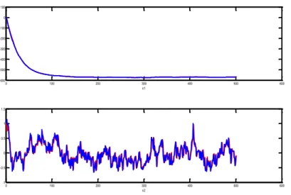
Other than comparison of the observation and the control variables, it is also important to see whether the estimated parameters converge to their population values. Figure 3 states that the estimated parameters in the exogenous labor income process, which follows AR(2), converge to their parameter values, which are 1.2 and -0.3, respectively.

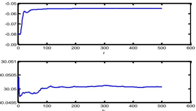
The estimated values for the real interest rate and the targeted consumption in the loss function can be seen in Figure 4. As it can be seen, while the interest rate is not very close, the targeted consumption is almost identical with its population value.

0 100 200 300 400 500 600 -600 -500 -400 -300 -200 -100 0 100 x1 0 100 200 300 400 500 600 -1 -0.5 0 0.5 1 1.5 x2

Figure 2: Comparison of the estimated and the actual values of the control variable ( Actual: Blue, Estimate: Red)

Figure 3: The estimated parameter values in the exogenous labor income process

Figure 4: The estimated values for the real interest rate and the targeted consumption

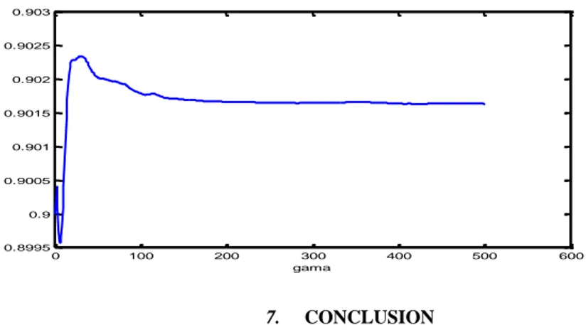
Finally, the evolution of the estimated value for the parameter in front of the investment in the loss function can be seen in Figure 5. While the population value is chosen to be as 1, the estimated value becomes steady at about 0.94, which is very close to its actual value.

0 50 100 150 200 250 300 350 400 450 500 -25 -20 -15 -10 -5 0 5

optimal control-red (observed control-blue)

0 100 200 300 400 500 600 1.1 1.15 1.2 1.25 ro1 0 100 200 300 400 500 600 -0.4 -0.35 -0.3 -0.25 -0.2 ro2 0 100 200 300 400 500 600 -0.09 -0.08 -0.07 -0.06 -0.05 r 0 100 200 300 400 500 600 30.0495 30.05 30.0505 30.051 b

Figure 5: The estimated value for the parameter in front of investment in the loss function

7. CONCLUSION

In this study, we develop a method to estimate the unknown parameters in an optimal control problem, where the objective (loss) function is quadratic and the constraints are linear. We show that, when the model is represented in state space form, the unknown parameters in the loss function and the system of equations can be simultaneously estimated by employing the extended Kalman filter.

In the second part of the paper, we conduct a simulation exercise to see the estimation accuracy of the introduced method. Using a simple intertemporal consumption-saving model for a representative household, we see that the estimated parameters are very close to the generated population values, which support our estimation method.

As a result, the estimation method, which is described in this paper, can be conveniently used for the purpose of simultaneously estimating the time-varying parameters in an optimal linear regulator problem.

Appendix 1 Kalman Filter Algorithm

Suppose that, when the observations

Y

n





y y

0

, ,...,

1

y

n



are given, forecasting the state vector

n

x

is denoted by xˆn nE x y y n 0, 1,...,ynE x Y n n, and the covariance matrix of the disturbance term is denoted by Pn nE(xnxˆn n)(xnxˆn n)Yn

In this circumstance, depending on the initial values

0 100 200 300 400 500 600 0.8995 0.9 0.9005 0.901 0.9015 0.902 0.9025 0.903 gama

0 0 1 0 0 1 ˆ P P x x    

The Kalman filter algorithm is given by the following algorithm:

1 1 1 1 1 1

ˆ

_{n n n}

ˆ

_{n n n n}

x

_

 

_

x

_{ }



B u

_{ } (A1) 1 1 ˆ ˆ _{n n n}ˆ n n n n n n x x  K _y H x  _ (A2)   1 1 1 n n n n n n n n n K P H H P H R        _  _ (A3) 



n n



 1 n n n n P  I K H P _ (A4) 1 1 1 1 1 1 n 1 1 n n n n n n n n

P

_

 

_

P

_{ }

 



_

G Q G

_{ }



_ (A5) Equation (3) is also known as the Kalman gain.

Appendix 2

Extended Kalman Filter Algorithm Suppose that

 

 

 

 

1 2 2 3 1 , , n n n n n T n n x K P n P n X K P P n P n L             _ _      

where K and P are Kalman gain and the covariance matrix of the extended state, respectively,

as stated in Ljung and Söderström (1985). Then, the updating equations will be:





1 n _n n _{n n n n n} n x F x G u K y H x (A6) 0

ˆ 0

x







1 ₁ n n L_n y_n H_n xn      _ (A7) 0 ₀  

 

 

 

 





1 1 1 2 2 12 T T T T T n n n n n n n n n n K  F P n H M P n H F P n D M P n D R S (A8)

 

 

 

 

1 2 2 3 2 T T T T T n n n n n n n n n

S



H P n H



H P n D



D P

n H



D P n D



R

(A9)

 



 

 



1 2 1 3 T T T n n n L n  P n H  P n D S (A10)





 

 

 

 

1

1

1 2 2 3 1 T T T T T T n n n n n n n n n n n

P n

 

F P n F



F P n M



M P

n F



M P n M



K S K



R

(A11)

 

1

0

0

( )

0

P

 







 

 

2

1

2 3 T n n n n n

P n

 

F P n



M P n



K S L

(A12)

 

2

0

0

P







 

3

1

3 T n n n

P n

 

P n



L S L

(A13)

 

3

0

0

P



P

Here, it is assumed that

 

n n F F 

 

n n G G  (A14)

 

n n H H 



n, n,



n n M M  x u and



, ,



 

 

M x u F x G u          _  _  (A15) and



n1, n



n D D   x

 

,

 

D x H x         _ _  (A16) REFERENCES

[1] Anderson, B.D.O. and J.B. Moore (1979), “Optimal Filtering”, Prentice Hall, 1979. [2] Bacchetta, P., Gerlach, S.(1997). “Consumption and credit constraints:international

evidence”, Journal of Monetary Economics, 40, 207-238.

[3] Favero, C. A, Rovelli, R.(2003), “Modeling and Identifying central bank preferences ”, Journal of Money , Credit and Banking, 35, 545-556.

[4] Grillenzoni C.(1993), “ARIMA Processes with ARIMA parameters”, Journal of Business and Economic Statistics, 11, 235-250.

[5] Kalman, R. E. (1960), “A new Approach to Linear Filtering and Prediction Problems”, Journal of Basic Engineering, Vol. 82; 35-45.

[6] Ljungqvist, L, H. Lustig, R. Manvelli, T.J. Sargent, S.V. Nievwerburgh, (2001), “Exercises in Recursive Macroeconomic Theory”, unpublished manuscript, Stanford University, Hoover Institution.

[7] Ljungqvist, L and T.J. Sargent (2000), “Recursive Macroeconomic Theory”, The MIT Press, Cambridge, MA.

[8] Ljung, L and T. Söderström (1985), “Theory and Practice of Recursive Identification”, The MIT Press, Cambridge, MA.

[9] Özbek, L. and M. Efe (2004), “An adaptive extended Kalman filter with application to compartment models”, Communication in Statistics, Simulation and Computation, 33:145-158.

[10] Özlale, Ü. (2003), “Price Stability US Output Stability: tales of federal reserve administrations, Journal of Economic Dynamics and Control”, 27,1595-1610.

[11] Özbek, L., Özlale, Ü.(2005), “Employing the extended Kalman Filter in measuring the output gap, Journal of Economic Dynamics and Control”, 29, 1611-1622.

[12] Salemi, M. (1995), “Revealed preference of the federal reserve: using inverse control theory to interpret the policy equation of a vector autoregression, journal of business and economic statistics”, 13, 419-433.

Current Address: Levent Özbek, Ankara University, Department of Statistics, Faculty of Science, 06100 Tandoğan, Ankara-TURKEY

E-Mail: ozbek@science.ankara.edu.tr

Current Address: Esin Köksal Babacan, Ankara University, Department of Statistics, Faculty of Science, 06100 Tandoğan, Ankara-TURKEY