The impact of small lot ordering on traffic congestion in a physical distribution system

Full Terms & Conditions of access and use can be found at

https://www.tandfonline.com/action/journalInformation?journalCode=uiie21

IIE TRANSACTIONS

ISSN: 0740-817X (Print) 1545-8830 (Online) Journal homepage: https://www.tandfonline.com/loi/uiie20

The impact of small lot ordering on traffic

congestion in a physical distribution system

KAMRAN MOINZADEH , TED KLASTORIN & EMRE BERK

To cite this article: KAMRAN MOINZADEH , TED KLASTORIN & EMRE BERK (1997) The impact of small lot ordering on traffic congestion in a physical distribution system, IIE TRANSACTIONS, 29:8, 671-679, DOI: 10.1080/07408179708966377

To link to this article: https://doi.org/10.1080/07408179708966377

Published online: 31 May 2007.

Submit your article to this journal

Article views: 64

The impact of small lot ordering on traffic congestion

in a physical distribution system

KAMRAN MOINZADEH1_{,TED KLASTORIN}1

and EMRE BERK2

1Department of Management Science. School of Business, Box 353200, University of Washington, Seattle, WA 98195-3200, USA

2Faculty of Business Administration, Bilkent University, Ankara, Turkey

Received September 1995 and accepted April 1997

In recent years, some managers and researchers have advocated reducing lot sizes by decreasing setup costs, arguing that smaller lot sizes improve quality while reducing inventory levels and associated holding costs. However, smaller lot sizes result in an increased number of shipments which, in turn, exacerbates traffic congestion. This results in longer delivery times and, thereby, higher inventory levels. In this paper we study the relation between lot sizes and traffic congestion by constructing a model with numerous retailers who share a common congested delivery road. Using a numerical example, we illustrate the model's managerial implications with respect to several factors, including lot sizes, traffic congestion, and inventory levels. Our findings suggest that in a physical distribution system, if there are a relatively large number of retailers, no single retailer has an incentive to increase batch sizes because one retailer's effect on reducing traffic congestion will be negligible. If all retailers increase their lotsizes, however, traffic congestion will be reduced and all retailers will experience lower costs.

1. Introduction

In this paper we study the relation between lot sizes and traffic congestion in a physical distribution system. The idea of reducing lot sizes has been popularized in recent years as part or the 'just-in-time' (lIT) philosophy de-veloped in the 1960s by Ohno, and first implemented by Toyota [1]. JIT proponents advocate reducing setup costs to improve flexibility and the ability to adapt quickly to changing demand. It is further argued that smaller lot sizes (ideally a batch size of one) will result in reduced inventory levels requiring less warehouse space and lower costs (see Zipkin [2] for a more comprehensive discussion of lIT philosophy and practice).

Smaller lot sizes, however, lead to more frequent shipments, which increase traffic congestion and result in longer delivery lead times and higher inventory levels. In addition, increased traffic congestion causes environ-mental degradation and negatively impacts road condi-tions and social welfare (For example, vehicle carbon dioxide emissions increased from 15% _{in 1975 to about} 20% in 1990 in Japan [3]. Also see NRC [4] for a dis-cussion of related issues in the USA.). These costs are causing managers and government agencies alike to re-consider the theory and practice of small lot ordering.

Negative consequences of lot size reduction have been described in numerous recent articles [5-8]. Referring to the Tokyo metropolitan area, Shiomi et al. [3] state bluntly that' ...the frequent movements of trucks under 0740-817X © 1997 "liE"

lIT create chronic traffic jams in large cities and pollute the environment'. Abrahams [9] quotes the director of basic chemicals at one of Japan's largest plastics manu-facturers, who stated that 'Acrylic sheet was infamous for small deliveries, even within the plastics industry. We were sometimes having to make deliveries three times a day. The costs were exorbitant. Not only did you have to cover the cost of freight, but you had to carry larger inventory too.'

In this research we study the impact of small lot or-dering on traffic congestion in a supply chain. Specifi-cally, we consider a physical distribution system with a number of retail outlets that share a common road for deliveries (the Interstate-5 corridor in the Seattle met-ropolitan area is an example of such a situation). We assume that demand at the retail outlets is random, and that fixed order costs are zero. Furthermore we assume that the speed of the delivery vehicles on the common road is a non-increasing function of the number of the vehicles on the road (i.e., the traffic density). This latter assumption implies that order lead times are random and depend on the number of vehicles on the road at any point in time.

We initially develop expressions for the operating characteristics of the system. Using these expressions, we show that when JIT ordering creates traffic congestion, the retailers can reduce their operating costs through a coordinated effort by increasing lot sizes (the solution adopted by the Japanese plastics industry). When such a

672

coordinated effort does not occur among retailers, there are implications for government agencies that can impose road fees (e.g., toll fees, usage fees, taxes). Such fees would reduce traffic congestion and its associated social, structural and environmental degradations while collect-ing money for road maintenance.

To the best of our knowledge this is the first work that studies the effect of small lot ordering on traffic conges-tion, order leadtimes and operating costs in a multi-lo-cation physical distribution system. Previous research in multi-echelon distribution system has studied systems where congestion is only a factor in the production pro-cess. In these situations, standard queueing models were used for modelling congestion [10-14]. Other related work includes studies between the batch size and pro-duction lead times in a single-facility production envi-ronment by Karmarkar [15] and Karmarkar et al. (16]. Assuming that production times are exponentially dis-tributed, the authors modelled the production facility as an M / M / I queue and showed that production leadtimes increase as smaller production batch sizes are used.

The rest of this paper is organized as follows. In Sec-tion 2 we describe the physical distribution system and outline the relations which enable us to evaluate the op-erating measures of such systems. Specifically, we initially compute the steady-state probability distribution of the order lead times for our model. Using results from multi-echelon inventory theory, we then find the probability distributions of the number of outstanding orders at each retailer and, subsequently, the. average total expected cost rate. In the Section 3 we introduce the functional relation between the speed of the vehicles on the road and the traffic density. In Section 4 we present the results of a numerical experiment that illustrates the impact of traffic congestion on lIT ordering by using the model developed in previous sections. Finally, we summarize our findings and discuss possible extensions of the basic model.

2. Specification of the physical distribution model Consider a physical distribution system consisting ofM

retailers sharing a common delivery road for their goods. Without loss of generality, we assume that all retailers (with index set 1

=

{I, ... ,

M}) .stock one product (but not necessarily the same product) and order u-nits from suppliers in integer multiples,

m.,

of a minimum allowable order quantity, bi(i E I). (The quantity b, is determined by packaging or freight considerations.) Inventories at all facilities are reviewed continuously and a

(Q,

R)ordering policy is used at each location; that is, when inventory positionI, (on-hand

+

on-order - backorders) reachesRi ,

retailer i places another order of size Qi [17], where Q,=mJb,.

Demand for the product occurs at the retailers according to a Poisson process with a mean rate Aj for

Moinzadeh

et al.

retailer i. If the retailer does not have sufficient units on hand to meet demand, a backorder occurs. For ease of exposition, we assume that retailers' orders are filled immediately by the suppliers (i.e., there are no order de-lays at the supplier). Therefore order leadtime is deter-mined only by the transit time to ship Qi units from the supplier to retailer i. To simplify the discussion, we will use Q to denote the vector of all order quantities (i.e., Q

=

(Qt,Q2, ... , QM))and R to denote the vector of all reorder points (i.e., R

=

(R1,R2,... ,RM ) ) .

To study the impact of lIT ordering, we assume that fixed order' costs are zero and that retailers order the minimum allowable batch size, b, (i.e., m,

=

1'V i E1).

This assumption is consistent with the goal of lIT or-dering [2] and the increased emphasis on EDI in supply chain management.

All orders are shipped on a common road to their re-spective retailers; the transit time on this road is denoted by the random variabler. The distance to be travelled by all vehicles on this common road is Y;vehicular speed is Un when there are n vehicles on the road (i.e., n is a measure of the traffic density). We assume that Un is a monotonically non-increasing function ofn.The common road, however, may only constitute a portion of the total distance from the suppliers to each retailer. Thus we as-sume that there is an additional distance to each retailer; this latter segment is travelled on a non-congested road and takes a known time, T; ('Vi EI). The total transit time(and, hence. the order leadtime) faced by retaileri,!i,

is then defined as t, = !

+

Ti.

2.1. Distrihution of order leadtimes

We note that traffic density is determined by the number of vehicles shipping goods to retailers as well as non-commercial traffic that may be using the common road. We will denote the average rate which th~ non-commer-cial traffic enters the common road by A; therefore the average rate of vehicle entry, A, to the common road is equal to

"'" Ai ... A= LQ.+A,

iEJ t

given that retaileri orders in batches ofQ;. If the number of retailers in the distribution system is relatively large arid/or the non-commercial traffic constitutes a significant portion of the total traffic to the road, the order arrival process to the road can be approximated by a Poisson process (see Feller [18] for a description, Albin [19] for extensive empirical tests that support the approximation, and Zipkin [10] for a general discussion and application of such an approximation). Therefore we approximate the entry of vehicles to the common road by a Poisson process with mean A.

To derive the probability distribution of the number of vehicles on the road (and, hence, the probability

distri-bution of order Jeadtimes), we let xn(t)

=

{XI(t), . . . , Xn(t)} denote the stochastic process that describes the

status of the vehicles on the common road at timet withn

vehicles on the road andx;(t)denotes the remaining dis-tance to be travelled by the ith vehicle on the road prior to t. Note that vehicles on the road are ordered on a FIFO basis; that is, 0 ~XI ~X2 ~ ... ~Xn ~ Y. We

de-rive expressions for the steady-state density of

X_{n ,Pn(XI, X2, ...}1x_{n) ,} and the steady-state probability of

havingn vehicles on the road,Pn , in the following

prop-osition.

E[b;(b; - 1)]

=

A;E(r;) ,

whereE(t;)is the second moment ofri.Itfollows that the variance ofb; can be expressed as

V(Oi)

=

(~YV(N)

+

G)

(1 -

~)E(N)

+

AiT;. (8)

Let B; and OHj denote the number of units backordered

and the number of units on-hand, respectively, at retailer

t.To evaluate the steady-state operating measures at each retailer, we note that

and

where K is a normalizing constant and is equal to

Proof: The details of the proof are described in Appendix

A. • In the absence of order costs, the expected total cost rate

TC;(Qi, R;) at each retailer is given by the sum of average holding and backorder costs

TCj(Q;,Ri )

=

h;{R; +!(Q;

+

1) - Ai[E(N)/A

+

1';l}

+

(hi

+

nj) E(B;) , (12)

If the objective is to minimizeTC(Q, R),then, for fixedQ,

the optimal reorder point at retailer i,

R;,

is the largest value ofR; that satisfies

R;+QJ 00 h

Q

L L

q;(k)

~

h.;

~.,

j=R;+l k=j+1 J

+ ,

TC(Q, R)

=

L

TC(Q;,R;). ;El

The relation between vehicular speed on a road and traffic density can be derived by considering the car-following behavior of single-driver-vehicle systems, or by directly studying the macroscopic behavior of platoons of vehicles 3. Vehicular speed on the common (congested) road £(OHj )

=

E([l; - £5;]+)

=

£(1;) - £(£5;)

+

E(B;)

=

R,

+

!(Q;

+

I) - A; [E(N)I1

+

Ii]

+

E(B;). (II)

where h; is the unit holding cost of an item at retaileriper unit time, and tt, is the unit backorder cost of an item at . retailer i per unit time. The .expected total cost rate for the system, TC(Q, R), is then the sum of the expected costs for all retailers; that is,

E(Bj )

=

E([bi - Ij]+), (9)

. where (x)+

==

max(O,x).

Since I; is uniformly distributed in [Rj

+

1,R;

+

Qi] [17],

. 1 Ri+Q, 00

E(Bi)

=

Qi

i~'1 ~(k

- j)qi(k), (10)

where q;(.) denotes the probability distribution of de-mand for retailer i.

Similarly, the expected on-hand inventory at retailer i

can be defined as follows:

(7) (6) (5) (4) (2) E(t) = E(N)/A L[A(1 - z)]= M(z) . V(r)

=

[V(N) - E{N)]/;? , E[b;J

=

(A;ll)E[N]

+

A;T; by (5). Furthermore we have (see [20]): and

It is also shown in Appendix A that the Laplace-Stieltjes transform of the travel time r of a vehicle on the common road, L(-), can be expressed in terms of the probabiJity-generating function of the number of vehicles on the common road, M(·), as follows:

K

=

{I

+

~(AY)"/[n!g

Vi]}

-1 (3)

For certain forms of Un (for example, Un= «]n for

n ~ 1, wherelXis a constant), one can obtain closed form

expressions for the steady-state probability distribution of the total travel time r of a vehicle on the common road. Furthermore, from (4), the expected value and variance of r are defined, respectively, as:

where N is the random variable denoting the number of cars on the common road.

Let l>; denote demand during leadtime at retailer i, Since demand at each retailer is assumed to be Poisson, then E[l>;] is equal to Ai E[t;] on the basis of Little's law. But t,

=

r

+

1';; therefore

Proposition 1. If limn_conu;

>

AY, then the steady-state distributions for Xn exists and

674

Moinzadeh

et al.

(13) and

{

no · ;.y( )no+1 }

E(N)=K Lng(n)(Ay)lI+ vono 2

71=0 no!f(no) (vono - lY)

(16) (15) (14) I 1 g(n)

=

n!f(n) - no!f(no) (novo)II-1l() . where Then p. _ { {(J.y)lI/[n!f(n)]}K, n - {(J.y)n

I

[no!f(no)(vono)II-1I0]}K , { 110 ( ) 110+1 } -I

K =

~

g(n) (J.Y)"

+

no!f(~)~:ono

_ J.Y)

The first two moments of the distribution of the number of vehicles on the road can then be expressed as

and

E(N2 ) = K { t n2_{g(n) (J.Y)"}

+

_J.Y(novo

+

_{J.Y)(novo)""3+} 1

} .

71=0 no!f(no) (novo - ;'Y)

(J7) Using(l6) and (17), we can calculate the mean and the variance of the number of orders outstanding at each retailer as defined by (7) and (8). Unfortunately, the specification of the probability distribution of the number of orders outstanding at each retaileri, qi('),is extremely complex when no

>

I. In this case, however, we can ap-proximate the distribution ofqi(') by using a two-par-ameter family. It can be easily shown thatE(~i)

<

V(~i)'

Therefore one alternative wilJ be to approximate the distribution ofqi(') with a negative binomial distribution with a mean and variance equal to E(b;) and V(£5;) and evaluate the operating measures of the retailers using(10) and (11). The negative binomial distribution has been previously used to approximate the steady-state distri-bution of the leadtime demand at various sites in the multi-echelon inventory literature and has been shown to be effective (see Svoronos and Zipkin [11], Graves [28]).

Furthermore, the average speed on the road is given by

1 00

V=--L

Vn P Il '

1 - Po71=1

where Vn is the vehicular speed when the traffic density is

equal to n.Note that the term 1/(1 - Po) appears because the average vehicular speed is calculated only for the in-stances when there are vehicles on the road.

The characteristics of the traffic model is illustrated in Fig. 1, which presents the relation between average speed,

V,and the road utilization ratio, p. This graph indicates that the average vehicle speed approaches zero asymp-toticaUy as the road utilization approaches unity (as ex-where Vfreeis the free, or equilibrium, vehicular speed as

the traffic density, n, approaches zero, and Vo is the speed at the critical density level no. To ensure continuity, we define

Vfree - Vo c t =

-no

Proposition 1 specifies a stability condition that must hold for a steady-state distribution for Xn to exist; that is,

lim nVIl

=

vono

>

;'Y .

11-00

11

f(n)

=

IT

(Vfree - cd) i=1

on a given road section. As Gazis et al. [21] have dem-onstrated, the two approaches yield similar speed-density relationships. The relations obtained suggest that vehicle speed on a single road at steady state is a monotonic decreasing function of traffic density.

Greenshields [22] was among the first researchers to study the empirical relation between speed and traffic density and proposed an inverse relation approximated by a linear function. In order to better capture the true traffic behavior, especially for high traffic densities, sev-eral nonlinear (polynomial, logarithmic, and exponential) relation have since been developed. The particular choice ofa relation depends on factors such as the geometry of the road segment and the nature of traffic flow. We refer the interested reader to Gazis[23], Gerlough and Huber [24] and Papageorgiou [25] for a summary of speed-density hypotheses and supporting empirical data.

As Ross [26] observed, one shortcoming of previously suggested models is that the common speed for the iso-velocic flow of traffic is either zero at some 'jam' density or approaches zero asymptotically as the traffic density increases. This assumption results in a non-ergodic queueing system in general and violates the stability condition stated in Proposition 1. Therefore we use a hybrid speed Function similar to the one defined by Smulders [27] and supported by Ross [26]. In this case, vehicle speed declines linearly asafunction of the number of cars at lower traffic density levels. If the traffic density surpasses a critical density level no, vehicle speed is re-duced in hyperbolic fashion. The assumed relation be-tween vehicle speed and traffic density can be described mathematically as

{

Vfree - anl 0

<

n ~ no;

Vn

=

_vono

I

_{n, n}

_>

_no;

On the basis of this condition, we let p denote the ratio .

lYIvono, which provides an effective measure of utiliza-tion for the common road. We use this measure in the numerical example described in the following section.

Using (13) and the results obtained in the previous section, we can determinePIl'the probability distribution of the number of vehicles on the road. Let

0.90 0.80 0.60 0 + - - -..,...--r----r-- - __- - __- 1 0.50 0.70 INC

Fig. 2. Expected total cost for JIT ordering and optimal batch ordering (T

=

0.75,b

=

10, rc/(1rt

+

h)

=

0.98).

- - - 0 - TCopt ---.- TCjlt

..

_{~ 100}

o

however, that we varied p in other numerical experi-ments; our results in all cases were similar to those re-ported here.

U sing these parameters, we examined anumber . of performance measures under various conditions; results are presented in Figs 2 and 3. In Fig. 2 we compare the expected total cost TC(Q, R) for lIT ordering (i.e., mini-mum batch sizes when

Qj

=

b,.) with optimal batch sizes for varying values of

INC.

(In this case we set

T

=

0.75,

b

=

10, and

n/{n

+

h)

=

0.98; however, similar results were found for other values of these parameters.) As the fraction of non-commercial traffic increases (i.e., as the contribution of the orders from the retailer group to the overall vehicle traffic decreases), the cost differential be-tween lIT ordering (denoted in Fig. 2 by TCjit) and op-timal lotsizing (denoted in Fig. 2 by TC'opt) diminishes. This is as expected; as the fraction of non-commercial traffic increases, the impact of increasing lotsizes on leadtimes is reduced. It should also be noted that, al-though expected total cost decreases as a function of

INC,

we are solving different inventory problems for each value of

INC.

Therefore the significance of Fig. 2 lies in the relative difference between the expected costs of JIT and optimal ordering, and not the absolute values of the total costs.

Fig. 3 illustrates the impact of lotsizing as a function of the size of the constant portion of the delivery leadtime,

T, when

INC

=

0.70, b

=

]0, and

n/(n

+

h)

=

0.98. (Again, similar results were found for other values of these parameters.) As Tincreases, the impact of lotsizing gets smaller because traffic congestion and resulting travel time play a less significant role in the overall delivery delays. This has location policy implications for both retailers and suppliers; the supplier-retailer pairs that are closer to each other experience the biggest impact of the congestion on the road. However, as the distance between suppliers and retailers increases, the time on the

con-200 ~---1.0 0.9 0.8 0.7 0.6 O-+--...----....---~-r---.----.---.I 0.5 7 0 . . . - - - . 50

Ai

=

0.99bno vo[l -

INc]/M Y

ViEI.

This value of p was chosen to highlight the traffic con-gestion effects as indicated in Fig. 1. It should be noted,

"D lD CD : 40 and CD 0) 30

e

CD > c( 20

Road utilization ratio, p

10

In order to better illustrate the tradeoffs and managerial implications between lotsizing decisions and traffic con-gestion, we present the results of a numerical experiment where we analyzed 1000 scenarios. In each scenario we assumed that M = 30 and that the retailers, having identical parameters, used equallotsizes. For all retailers

i EI, we fixed hi

=

h

=

1 and set the ratio Tr.j/(nj

+

hj)

=

n/(n

+

h) to values (0.90,0.95,0.98,0.99). Furthermore we varied the constant portion of the de-livery lead times and set

1i

=

T

=

(0.1,0.25,0.5,0.75,1.0). To allow for differences in product attributes, we varied the number of items in a minimum shipment, and set all hi

=

b

=

(1,5,10,25,50).

With respect to the common road, we set Vfree

=

70, Vo

=

60,no

=

5, and Y

=

5. To investigate the impact of non-commercial traffic on road congestion, we varied the fraction of non-commercial traffic,

INC,

on the common road from 0.50 to 0.95 in increments of 0.05. Finally, the values ofAi (average demand at the ith retailer) were set for an retailers at a value such that the road utilization ratio p= AY/vo no was 0.99 when lIT ordering was used (i.e., when

Qj

=

bi)' This implies that

I

=

O.99(no vo)/Nc/Y

pected from the stability condition). For the value of

p

=

0.99,which we use in the numerical example reported in the following section, Fig. 1 indicates that the average vehicular speed at that level of congestion is approxi-mately 10 krn/h,

4. Numerical results

Fig. 1. Average speed, ii, plotted against the road utilization ratio, p(Vfree

=

70,Vo

=

60,no

=

5, and Y

=

5).

Fig. 3. Expected delivery leadtime, E{r), plotted against the

constant leadtime, T (INC

=

0.70,b= 10,tr/{n

+

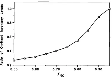
h) = 0.98).

Fig. 4. Ratio of on-hand inventory levels under lIT practice

and optimal ordering levels (T = 0.75,b= 10,n/{n

+

h)

= 0.98).

Acknowledgements

[1] Monden, Y. (1983) Toyota Production System. Industrial Engi-neering and Management Press, Norcross, GA.

[2] Zipkin, P. (1991) Does manufacturing need a JIT revolution?

Harvard Business Review,January-February. 4-10.

l3] Shiorm, E., Nomura, H" Chow, G. and Niiro, K. (1993) Physical distnbunon and transportation In the Tokyo metropolitan area.

The Logistics and Transportation Review,29 (4), 335-356. [4] NRC (1995) Expanding Metropolitan Highways: Implications for

Air Quality and Energy Use, Transportation Research Board,

National Research Council, Washington, D.C. References

M oinzadeh et al.

5. Conclusions and extensions

In this paper we studied a physical distribution system where a number of retailers share a common congested road. Assuming that order costs are negligible, we first developed a model for the traffic flow on the congested road. Using results from multi-echelon inventory theory, we derived the probability distributions of the number of outstanding orders at each retailer and, subsequently, the average total expected cost rate.

Our results indicate that ordering minimum batch sizes, even when there is no fixed cost associated with placing an order, may not be optimal in terms of minimizing total expect cost when road congestion is present. Aside from the operating cost perspective of the retailers, traffic congestion has public policy implications as well. As the traffic intensity increases due to commercial use, the travel time of all vehicles on the road increases. Other negative externalities occur such as degradation in road conditions and environmental pollution.

It is interesting to note that, if there are a relatively large number of retailers, no single retailer has an incentive to increase batch sizes because one retailer's effect on re-ducing traffic congestion is negligible. If all retailers in-crease their lotsizes, however, traffic congestion is reduced and all retailers experience lower costs. Given the envi-ronmental benefits and other externalities, this may be justification for imposing tolls on certain congested roads. The model presented in this paper could be used as a starting point for determining the magnitude of such tolls.

This research was supported in part by research grants to K.M. and T.K. from the School of Business and the Program in Engineering and Manufacturing Manage-ment (PEMM) at the University of Washington, and the Burlington Northern/Burlington Resources Foundation. Additional support was provided by a grant from the

Washington state Department of Transportation to the second author. The authors also acknowledge the anon-ymous reviewers for their helpful suggestions.

en '; _1.0 > At ..J ~ 0 0.8 E CD >

=

'a _0.6 c co X C 0 '0 0.4 ~ C; a: 0.2 0.50 0.60 0.70 o80 090 INC 676 CD .§ 0.9 ;; ra CD ...J CD 0.8 Eft co G; > cr: c _0.7 CD

•

III ~ u

=

0.6 At Eft ClI C CD 0.5

e

CD _{0.0 0.2 0.4 0.6 0.8 1.0} Q. T

gested road becomes a smaller fraction of the total lead time, thereby having a smaller impact on batching decisions.

One of the cited benefits of lIT is that it reduces inventory and associated holding costs. To investigate the impact of congestion under lIT practice, we ex-amined the on-hand inventory levels. In this case, T

=

0.75, b

=

10, and n/(n

+

h)

=

0.98. Fig. 4 illus-trates the ratio of the on-hand inventory levels under lIT practice and optimal ordering as a function of the fraction of non-commercial traffic on the congested road, INC. We note that the on-hand inventory levels are significantly lower when a retailer facing congestion deviates from lIT and orders in batch sizes larger than the minimum allowable shipment size.

[5] Jackson, T. (1991) Flexible response to delivery dilemma comes just in time. The Independent, May 10.

[6] Takada, K. (1991) Just-in-time delivery sits at the crossroads.The Daily Yomiuri, May 12.

[7] Cullison, A.E. (1992) Congested roads in Japan thwart just-in-time efficiency. Journal of Commerce, March 16.

[8] Bleakley, F. (1994) Just-in-time inventories fade in appeal as the recovery leads to rising demand. Wall Street Journal, October 25.

[9] Abrahams, P. (1994) Just in time now just too much - Japan's plastics suppliers are leading a revolt against the much praised management tool.Financial Times, March 30, p. 17.

[10] Zipkin, P. (1986) Design and control of stochastic, multi-item batch production systems. Operations Research, 34, 91-104.

(II] Svoronos, A. and Zipkin, P. (1988) Estimating the performance of multi-level inventory systems. Operations Research, 36 (1), 59-72.

[12] Deuerrneyer, B. and Schwarz, L.B. (1981) A model for the anal-ysis of system service level in warehouse/retailer distribution sys-tems: the identical retailer case, in Multilevel Production/Inventory Con trol (TIMS Studies in Management Science vol. 16), Schwarz, L.

(ed.), Elsevier, New York, pp. 163-193.

[13] Moinzadeh, K. and Lee, H.L. (1986) Batch size and stocking levels in multi-echelon repairable systems. Management Science,

32, 1567-1581.

[14] Lee, H.L. and Moinzadeh, K. (1987) Two-parameter approxi-mations for multi-echelon repairable inventory models with batch ordering policy.lIE Transactions 19 (2), 140-149.

[\5] Karmarkar, U. (1987) Lot sizes, lead times and process in-ventories.Management Science, 33, 409-418.

[16] Karmarkar, U., Kekre, S. and Kekre, S. (1985) Lotsizing in multi-item multi-machine job shops.lIE Transactions, 17, 290-298.

[17] Hadley, G.J. and Whitin, T.M. (1963) Analysis of Inventory Sys-tems, Prentice Hall, Englewood Cliffs, N.J.

[18] Feller, W. (1971) An Introduction to Probability Theory and Its Applications, vol. 2, Wiley, New York.

[19] Albin, S. (198]) On Poisson approximations for superposition arrival processes in queues. Management Science, 28, 126-137.

[20] Marshall, K.T. and Wolf, R.W. (1971) Customer average and time average queue lengths and waiting times. Journal of Applied Probability, 8, 535-542.

[21] Gazis, D.C., Herman, R.S. and Potts, R.B. (1959) Car-following theory of steady-state flow.Operations Research, 7, 499-505.

[22] Greenshields, B.D. (1934) A study of traffic capacity.Proceedings of the Highway Research Board, 14,448-474.

[23] Gazis, D.C. (ed.) (1974) Traffic Science, Wiley, New York.

[24] Gerlough, D.L. and Huber, M.J. (1975) Traffic Flow Theory.

Transportation Research Board Special Report no. J65, Wash-ington, D.C.

[25] Papageorgiou, M. (ed.) (1991)Concise Encyclopedia of Traffic and Transportation Systems, Pergamon Press, Oxford.

[26] Ross, P. (1988) Traffic dynamics. Transportation Research Board,

228,421-435.

[27] Smulders, S. (l990) Control of freeway traffic flow by variable speed signs. Transportation Research, 24B, 111-132.

[28] Graves, S.G. (1985) A multiechelon repairable inventory item with one for one replenisment. Management Science, 31,

1247-1256.

[29] Gnedenko, B. and Kovalenko, LN. (1968) Introduction to Queueing Theory, Israel Program for Scientific Translations,

Je-rusalem.

[30] Schmidt, C.P. and Nahmias, S. (1985) (S - I,S)policies for per-ishable inventory.Management Science, 31, 719-728.

[31] Moinzadeh, K. (1989) Operating characteristics of the (S - 1,S)

inventory system with partial backorders and constant resupply times. Management Science, 35, 472-477.

[32] Moinzadeh, K. and Schmidt, C.P. (199)) An (8 - 1,S)inventory system with emergency orders. Operations Research, 39, 308-321.

[33] Courant, R. and John, F. (1989) Introduction 10 Calculus and Analysis, vol. I, Springer-Verlag, New York.

[34] Stidham, S., Jr (1970)L=-tW:adiscounted analogue and a new proof.Operations Research, 20, 708-732.

[35] Cox, D.R. (1967) Renewal Theory, Methuen, London.

[36] Gross, D. and Harris, C.M. (1985) Fundamentals of Queueing Systems, Wiley, New York.

Appendix A

Proof of Proposition 1

LetPlI(t,xll • • •,xlI) denote the probability density of the

road status's being XlIat time t. We derive the system of partial differential equations and their boundary condi-tions that describe the status of the vehicles of the road. Our approach is similar to that employed by Gnedenko and Kovalenko [29], Schmidt and Nahmias [30], Mo-inzadeh [31]and Moinzadeh and Schmidt [32].

Case 1:n

=

O. Let LI

>

0 be a small number. In order to have no vehicles on the road at time t

+

LI, either there were no vehicles on the road at t and no new vehicle entered the road during (t,t

+

LI) or there was one vehicle on the road at time t travelling at a speed VI with a

re-maining distance to be travelled less than viLi.This means that by time t

+

LI, the vehicle has reached its destination and therefore left the road. Thus we have:

Po(t

+

L1, .)

=

(I - ALI)Po (t, .)

.dVI

+

(l -lL1)

J

PI(t,

o«

+

o(L1). (A I)

o

Using the integral mean value theorem ([33], pp.

139-143), we can write(AI) as:

[po(t

+

LI,') - Po(t, .)]/LI

=

-AfJo{t,·)

+

VIPI

(t,

e)

+

o(LI), where 0~ e

s

LI.

Letting LI ---+ 0 and assuming that a steady-state solution exists, we get:

(A2) Case 2: n

>

0, Xl

>

0 and X_n

<

Y. To be at X_n at time

t

+

LI, one of the following should happen:

(1) There were n vehicles on the road at time t with remaining distances to be travelled equal to (Xl

+

Llv_{n , .•.},Xn

+

Llvn ) and there were no new

entries to the road during (t,t

+

LI).

(2) There were (n

+

1) vehicles on the road at time t with remaining distances to be travelled equal to

«(,Xl

+

LlVn+l, ...,Xn

+

LlvlI+d,where 0 ~( ~ L1vn+l,

and there were no new entries to the road during

(t,t

+

11). This means that the first vehicle on the road reaches its destination and leaves the road by

678

Thus, we have: Pn(t

+

Lf,xt, ...,xn)

=

(I - l.d )Pn(t,Xl

+

LfV_{n, ...},X_n

+

.dV_n)

+

(1 - lLi)

.dVII+1

X

J

P.+I

(t.

"XI

+

LlV.+I, ... •X.

+

Llv.+tldC

+

o(Ll).

o

Using the integral mean value theorem, adding and subtracting successive terms and letting .d ~ 0 and t~ 00, we get:

,lP.(XI, . . .• x.) -

t

?~ =

V.+IP.+I(O.XI •...,x.). (A3) ;=1 UX,

Next we derive the boundary conditions for the above system of partial differential equations. Consider

[n,

(I(r), . . . ,'n(t)]to be the position of a particle at timet located in the region 0~

'I

(t)

s ...

~ 'net) ::s; Y. The motion of the particle is discontinuous when a new de-livery vehicle enters the road (a new order is placed). The boundary conditions are derived by considering such discontinuities. Define:

Qn(t,xl, ,Xn-I~Y)

=

J

7'

j

P.(t,

C... .. ,C.)dC•.. ·dC..

(A4)

.x\-/) Xn-I-[) y-/)

where {) ~0 is a small number. Qn(t,XI, ...,Xn-I,Y) re-presents the probability mass in a neighborhood of the boundary (XI, . . .,Xn-1,Y). .

Applying the mean vaJue theorem, for some

o

~ 6; ~ ~ (i

=

1, ...,n), we get:

Qn(t,xI, ...,Xn- !,Y)

=

bnpn(t,xl - £1, . . . ,Y - En)

+

o(bn). (A5)

Moinzadeh

et al.

VnPn(XI, . . . ,Xn-),Y)

=

A.pn-l (Xl, . . .,Xn-1). (A7)

Assuming that a steady-state solution exists, a solution to the above differential equations and their boundary conditions is:

whereK is the normalizing constant.

The steady-state probability of having n vehicles on the road is now obtained as

y y y

r;

=

JJ... J

P.(XI,.··.x.)dx, .. .dx2dx]

o x\ .xlt-I

(A8) Finally, the normalizing constant, K, is found

bysum-ming the probabilities to unity, which yields (3). For the steady state solution to exist, K must be finite. This in turn means that

(A9) Substituting(A7) into (3) Jim_{n_ oo}no;

>

lY as the condi-tion for the existence of the steady-state solucondi-tion. •

6. Derivation of (4)

To prove that (4) holds, we first focus on the times when a vehicle departs the road. Let:

p~D)= steady-state probability of having n

vehicles on the road as a vehicle departs the road Furthermore, Qn(t

+

b/vn,xt, .. .,Xn-I,Y) b = l -Vn xl-e5+e5(vn_d vll )

X,,_I +/)(Vn-IIv,,)

J

P.-I(t,CI,' ..• C.-I)dC.-1 ... dCI' X,,-I-e5+{)(VI l - l / vn )

Then

p(D)

n

Pr{a departure is about to occur and there are n

+

1 vehicles on the road} Pr

{a

departure is abou t to occur}

y y y

Vn+l

J

f···

J

pn+l(O,XI, ...lXn)dx, ... dx2dx.

oXI Xn

00 YY Y

E

Vi+J

J

J...

J

P;+I(0,x}, . . .,Xi)dr, ...dx2dx l

;=0 0XI x,

Using the Taylor expansion together with the mean value theorem, Qn(t

+

b/vn,Xt, ... ,Xn-I,Y) can be also written as

Qn(t

+

fJ/vn, XI, .•. ,Xn-l,Y)

=

().bn/Vn)Pn_J(XI -61, .. .,Xn-I -En-I)+o(bn) . (A6)

Equating (A5) and (A6), dividing by bn and letting t~ 00, weget:

Applying the results from Proposition 1, we get:

AVn+l[(A.y)n/

(n!

fl

Vj)]

K n

p(D)

=

1=1

=

(A.Y) K

=

Pn.

n

A

f:

Vi+1

[(AY);/

(i!

in

Vj)]

K n!

D

Vj

J=O 1=1 }

(All) Therefore we conclude that the steady-state probability-of havingnvehicles on the road at a departure point is equal to the steady-state probability of havingn vehicles on the road at an arbitrary point in time.

Because the vehicles leave the road on a FIFO basis, arrivals to the road are Poisson and, as shown in Prop-osition 1, Pn(Xl,".'Xn) is independent of (XI, ...,x_n);

then, from the law of total probability, we can express

pJD) (and thusPn) as:

00

p.

=

p(D)

=

J

p(D)dF(t)

n n nIt '

o

where p~~) denotes the steady-state probability that a departing vehicle leaves n vehicles on the road given that its travel time on the road was t time units, andF(·) is the cumulative distribution function of time spent on the road, r, by a vehicle.

Furthermore, assuming that the processXn , as defined.

before, is ergodic (that is, limn_ oono;

>

lY), as shown in

Stidham [34], Little's law must hold. Thus we conclude (Cox [35], pp. 45-46) that D

(At)n

Pnlt

=

-,-exp(-At) n. and 00

r;

=

J

(~r

exp(-At) dF(t),

o

which, following Gross and Harris ([36], pp. 272-273), results in (4).

Biographies

Kamran Moinzadeh is the Burlington Northern/Burlington Resources Professor of Manufacturing Management, Professor of Management

Science, and the co-director of Program in Engineering and Manu-facturing Management (PEMM) at the University of Washington. He received his B.A. in Computer Science from the University of Cali-fornia, San Diego, his M.S. in Operations Research, and his Ph.D. in Industrial Engineering from Stanford University. Dr Moinzadeh's

publications have appeared in Management Science, Operations Re-search, Naval Research Logistics, European Journal of Operational Research, and lIE Transactions. His research interests include pro-duction/operations management, inventory and supply chain man-agement, and quality management. Dr Moinzadeh is a member of INFORMS and lIE. He is currently the editor of the Department of Inventory inlIETransactionsand is serving as the Associate Editor for

Operations Research.He has been the consultant to Microsoft Corp., Starbucks Coffee Inc., and Boeing Computer Services.

Ted Klastorin is the Burlington Northern/Burlington Resources Pro-fessor of Operations Management and Chair of the Department of Management Science (School of Business), and Adjunct Professor in the Department of Health Services (School of Public Health and Community Medicine) at the University of Washington, Seattle, Washington. Professor Klastorin also holds an appointment as senior research fellow at the IC2 Institute, The University of Texas, Austin, TX. He holds a B.S. degree from Carnegie-Mellon University (1969) and a Ph.D. from the University of Texas at Austin (1973). Professor Klastorin's research interests include logistics, quality control/assur-ance, project management, inventory, scheduling and queuing 'prob-lems in manufacturing and service organizations. Current research projects include stochastic line balancing problems, resource allocation in project management, and the impact of the Internet on company performance. His recent articles have appeared in llE Transactions,

Journal of Applied Psychology, and Management Science. Professor

Klastorin has consulted with numerous organizations, including Boe-ing, Microsoft, and Fluke Corp. He is a member of INFORMS and lIE, and serves as a member of the editorial boards of the Journal of Manufacturing and Service Operationsand lIETransactions.

Emre Berk is Assistant Professor at the School of Business, Bilkent University, Turkey. Dr Berk received his B.Sc. in Mechanical Engi-neering at Bogazici University, Turkey and his M.Sc. in Mechanical Engineering at Washington State University. He received his M.B.A. and Ph.D. in Operations Management at University of Washington. His research interests include supply chain management and stochastic models in health care applications. He is a member of INFORMS.