FACTORY LEVEL PREVENTIVE MAINTENANCE IN
TURKISH AIR FORCE
a thesis
submitted to the department of industrial engineering
and the institute of engineering and sciences
of bilkent university
in partial fulfillment of the requirements
for the degree of
master of science
By
Nuriye ¨
Unl¨u
August 2006
I certify that I have read this thesis and that in my opinion it is fully adequate, in scope and in quality, as a thesis for the degree of Master of Science.
Prof. M. Selim Akt¨urk(Principal Advisor)
I certify that I have read this thesis and that in my opinion it is fully adequate, in scope and in quality, as a thesis for the degree of Master of Science.
Asst. Prof. Alper S¸en
I certify that I have read this thesis and that in my opinion it is fully adequate, in scope and in quality, as a thesis for the degree of Master of Science.
Asst. Prof. Yavuz G¨unalay
Approved for the Institute of Engineering and Sciences:
Prof. Mehmet Baray
ABSTRACT
FACTORY LEVEL PREVENTIVE MAINTENANCE IN
TURKISH AIR FORCE
Nuriye ¨
Unl¨u
M.S. in Industrial Engineering
Supervisor: Prof. M. Selim Akt¨urk
August 2006
In this thesis, we study the Factory Level Preventive Maintenance Problem (FLPM) experienced by Turkish Air Force (TUAF). This problem is a specific case of Nonpreemptive Resource Constrained Multiple Project Scheduling with Mode Selection (NRCMPSMS); allocation of limited resources to competing activities of multiple project of different types in which the duration of an activity is determined by the mode selection and the activity flow is dependent on the type of the project. The objective is to determine the start (finish) time and the mode of each project’s each activity so that the minimal total weighted tardiness and total incurred cost are obtained. We proposed a heuristic for this problem definition which is composed of two phases and apply it to a real life problem experienced by TUAF. In the first phase, the aim is to construct an initial schedule with minimum total weighted tardiness and in the second phase, this schedule is improved in terms of total incurred cost by the mode selection exchanges. Since the activity due date information is not available but required in prioritization of the activities, we develop five FLPM specific activity due date estimation methods. We run the proposed heuristic for three different weight
figures which are determined by the Analytic Hierarchy Process and the one being used by TUAF. In addition, we study the influence of the release and the due dates of the aircrafts on the objective functions. We propose a determination method for each of the release and the due dates that aims finding the tightness levels of these two parameters. The release date determination method that we propose relates the arrival rate of the aircrafts with the utilization of the bottleneck resource whereas the due date determination method that we propose relates the due dates of the aircrafts with the fraction of the number of tardy jobs in percentages. We investigate the performance of the activity due date estimation methods in terms of the objective functions and the computational effort required by the tightness levels of the release and the due date that are found by the determination methods that we propose.
Keywords: Resource constrained project scheduling, multiple projects, mode selection, project types, weighted tardiness.
¨
OZET
T ¨
URK HAVA KUVVETLER˙INDE FABR˙IKA SEV˙IYES˙I
KORUYUCU BAKIM
Nuriye ¨
Unl¨u
End¨ustri M¨uhenlisli˘gi Y¨uksek Lisans
Tez Y¨oneticisi: Prof. Dr. M. Selim Akt¨urk
A˘gustos 2006
Bu tezde T¨urk Hava Kuvvetleri’nin (THK) tecr¨ube etti˘gi Fabrika Seviyesi Koruyucu Bakım (FSKB) problemini ¸calı¸stık. Mod Se¸cimli, Kaynak Kısıtlı ve Kesintisiz C¸ oklu Proje C¸ izelgelemesi Probleminin ¨ozel bir hali olan bu problemde, kısıtlı kaynakların de˘gi¸sik t¨urden projelerin birbiriyle rekabet eden aktivitelerine tahsis edilmesi konu alınmı¸stır. Buna ek olarak bu problemde, aktivitelerin s¨ureleri mod se¸cimi ile belirlenmektedir ve aktivite akı¸sı proje t¨ur¨une ba˘glıdır. Bu problemde hedeflenen sonu¸c, en az a˘gırlıklı toplam gecikmeyi sa˘glayarak, her projenin her aktivitesinin ba¸slangı¸c ve biti¸s zamanını ve se¸cilen modu belirlemektir. Bu problemin ¸c¨oz¨um¨u i¸cin iki fazdan olu¸san bir sezgisel y¨ontem ¨onerdik ve bu sezgisel y¨ontemi THK’nın tecr¨ube etti˘gi bir probleme uyguladık. Birinci fazda ama¸c, minimum toplam a˘gırlıklı gecikme zamanına sahip bir ¸cizelge elde etmektir ve ikinci fazda ama¸c bu ¸cizelgeyi mod se¸cim de˘gi¸simleriyle toplam olu¸san maliyet a¸cısından iyile¸stirmektir. Aktivitelerin ¨onceliklendirilmesinin gerekmesi, ayrıca bu aktivitelerin istenilen biti¸s zamanı bilgisinin elimizde olmaması nedeniyle, FSKB’ye ¨ozel ve aktivitelerin istenilen biti¸s zamanını tahmin eden be¸s adet metod geli¸stirdik. ¨Onerilen sezgisel y¨ontemi, ikisi Analitik Hiyerar¸si
Metodu ile belirlenmi¸s ve birisi THK tarafından kullanılmakta olan ¨u¸c de˘gi¸sik a˘gırlık fig¨ur¨u i¸cin ¸calı¸stırdık. Bununla birlikte, u¸cakların bırakılma ve istenen bitme zamanı parametrelerinin hedefler ¨uzerindeki etkilerini ¸calı¸stık. Ayrıca, u¸cakların bırakılma ve istenen bitme zamanı parametrelerinin sıklık seviyelerini bulmayı ama¸clayan belirleme metodları da ¨onerdik. Onerdi˘gimiz u¸cakların¨ bırakılma zamanını belirleme metodu, u¸cakların varı¸s sıklık de˘geri ile dar bo˘gaz olan kayna˘gın kullanım oranını ili¸skilendirirken, u¸cakların istenen bitme zamanını belirleme metodu u¸cakların istenen bitme zamanlarını geciken u¸cakların y¨uzdesi ile ili¸skilendirmektedir. Aktivitelerin istenilen bitme zamanı tahmin metodlarının hedefler ve hesaplama zamanı a¸cısından performanslarını, u¸cakların bırakılma ve istenen bitme zamanları sıklık seviyelerine g¨ore ara¸stırdık.
Anahtar S¨ozc¨ukler: Kaynak kısıtlı proje ¸cizelgeleme, ¸coklu proje, mod se¸cimi, proje t¨urleri, a˘gırlıklı ge¸c kalı¸s.
ACKNOWLEDGEMENT
I would like to express my sincere gratitude to Prof. Selim Akt¨urk for his supervision and encouragement in this thesis work. I am grateful for his invaluable contribution to my graduate study. His patience and understanding let this thesis come to an end.
I am indebted to Asst. Prof. Asst. Alper S¸en and Asst. Prof. Yavuz G¨unalay for accepting to read and review this thesis and for their valuable comments and suggestions.
I would like to thank to Hakan G¨ultekin and Yavuz Bey from BCC for sharing their technical knowledge with me throughout my graduate study.
Finally, I would like to express my deepest gratitude to my son Ahmet Selim for being a well-behaved baby, my husband Mehmet for reviewing my thesis from an academician point of view, my mother Saygı and my father Alaattin for their prayers, and Meryem Hanım for looking after Ahmet Selim very well. It would be hard to bear with all this thesis time without them and their continuous morale support, love and understanding.
And to everyone, who trusted, helped and encouraged me throughout my studies.
Contents
1 Introduction 1
2 Literature Review 5
2.1 Single Project Scheduling with Limited Resources . . . 7
2.2 Resource Constrained Project Scheduling with Multiple Modes . . 12
2.3 Multiple Project Scheduling with Limited Resources . . . 19
2.4 Motivations for this study . . . 22
3 The Factory Level Preventive Maintenance Problem in Turkish Air Force 23 3.1 The Factory Level Preventive Maintenance (FLPM) Problem . . . 24
3.2 Preliminaries and Problem Definition . . . 29
3.3 Modelling the Problem . . . 31
3.4 A Heuristic Procedure for the FLPM Problem . . . 34
3.4.1 Generation of the initial feasible schedule . . . 34
3.4.2 Improvement of the initial feasible schedule . . . 41
3.5 A Numerical Example . . . 44
3.6 Conclusion . . . 55
4 Numerical Study 64 4.1 FLPM Specific Data . . . 65
4.2 Experimental Setting . . . 70
4.3 Results for the FLPM Problem Experienced by TUAF . . . 82
4.5 Results for Improvement Phase . . . 92 4.6 Analysis of Results . . . 95 4.7 Conclusion . . . 107
5 Conclusion 114
A Results, Descriptive Statistics 129
List of Figures
3.1 Precedence diagram of a F4 aircraft . . . 26
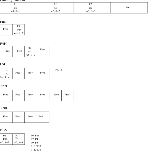
3.2 Existing work load . . . 45
3.3 The work load at t=1 . . . 57
3.4 Work load after resource assignment . . . 58
3.5 Work load at t=2 . . . 59
3.6 Initial Feasible Schedule . . . 60
3.7 The Gantt Chart before and after phase 2 for P11 . . . 61
3.8 The Gantt Chart after phase 2 . . . 62
3.9 Total incurred cost obtained after each mode selection exchange . 63 4.1 Precedence diagram of a F16 aircraft . . . 70
4.2 Existing work load in the common shelters . . . 110
4.3 Existing work load in the PAC type shelters . . . 111
4.4 Release date coefficient versus utilization level of the bottleneck shelter diagram . . . 112
4.5 Due date coefficient versus fraction of the number of tardy projects in percentage diagram . . . 113
Chapter 1
Introduction
Resource Constrained Project Scheduling (RCPS) problem has been an inter-esting topic in the past decades since it is encountered in many areas with unlimited number of problem types varying from management to operational level situations. It is concerned with the allocation of limited resources over time to perform a collection of activities as stated by Dorndorf [18]. Meanwhile, the projects consists of activities between which a precedence relationship exists. While allocating the resources, specific objectives are taken into account such as the minimization of total completion time or total cost. Assignment of limited resources to competing activities is in fact determining the exact activity start and finish times.
The mathematical model representations for the RCPS are initially formed in the mid sixties by Bowman [10] and Huber and Patterson [43]. However, the computational effort for finding an optimal solution usually grows exponentially with the problem size, thus the underlying problems are difficult to solve. Therefore, different solution procedures in the literature have been launched recently in the late nineties. Even the question for the existence of a feasible schedule can be answered with exponentially growing effort as stated by Dorndorf [18]. In practice, this problem is even more difficult to solve since the actual conditions under which a schedule will be executed change over time. According to the survey by Fox and Ringer [20], less than 5% of the time spent in practice on
scheduling is for developing new schedules, while 95% of the time spent is revising and maintaining schedules based on daily progress and changing environment. The difficulty arises because of the combinatorial nature of the problem and the difficulty in putting the schedules into practice because of the changing conditions lead the project managers to develop special case solutions. However, there are unfortunately no problem specific studies in the literature. Nevertheless, industry specific heuristics can serve as more qualified decision tools. One of the areas this situation observed is the maintenance shops of aircrafts.
In this study we will consider Factory Level Preventive Maintenance (FLPM) of the aircrafts belonging to Turkish Air Force (TUAF) and propose a new solution procedure to this real life problem. TUAF has five war aircraft configurations which are F16, F5, F4, T37, and T38. All the aircrafts of these configurations are sent to Military Supply Point in Eskisehir in predetermined periods for FLPM. It is important to notice that the aircraft is unavailable during FLPM as expected. Since one of the main objective of TUAF is having as many available aircrafts as possible in case of a arising war, TUAF aims minimizing the time elapsed to complete the FLPM. A task plan exists for FLPM where the order of the operations, the time, and the resources required to perform each operation are gathered in. The resources required are the docks in the shelters and the workers who are certified by skill levels 7, 5, and 3. In addition, different FLPM task plans are used for each aircraft configuration.
At the beginning of each year, the fleets prepare a list of the aircrafts which has FLPM due in that year. These lists also include release and due dates of FLPM for each aircraft. The Military Supply Point (MSP) in Eskisehir is asked for the cost, which consists of only the labor cost, to complete all the FLPMs of the aircrafts in the lists. After estimating the required cost, MSP could be asked for a rescheduled FLPM list with a decreased cost but an increased total weighted tardiness and again the MSP calculates the required cost. This cycle is carried out till MSP ends up with a reasonable cost estimate.
The FLPM is a special case of Nonpreemptive Resource Constrained Multiple Project Scheduling with Mode Selection (NRCMPSMS) [38]. A set of activities
(υ = {1, 2, . . . , J}) of a set of weighted projects (β = {1, 2, . . . , I}), for which due dates are set, compete for the shared resources, and are to be processed in one of multiple possible execution modes. These modes differ with respect to their processing time. The objectives that are considered are minimizing the total weighted tardiness and the total required cost. Here, the projects are the FLPM of each arriving aircraft, the resources are the workers and the docks in the shelters, and the modes are the worker skill levels.
For this real life problem, we propose a new solution procedure which consists of two phases. In the first phase, an initial feasible schedule that has minimal total weighted tardiness is generated. In the second phase, this initial feasible schedule is improved in terms of total cost required. The proposed heuristic requires the activity due date information which is not available in the existing FLPM problem. Therefore, five activity due date estimation methods are developed considering the properties of the FLPM problem and the method developed by Vepsailanen and Morton [58] is also studied. For this problem definition, we also develop a release and a due date determination methods. The methods that we propose aim finding the tightness levels of these two parameters. The release date determination method that we propose relates the arrival rate of the aircrafts with the utilization of the bottleneck shelters whereas the due date determination method that we propose relates the due dates of the aircrafts with the fraction of the number of tardy jobs in percentages. Then, we solve the FLPM problems using different tightness levels of the release and the due dates generated by the release and the due date determination methods that we propose. Then, we investigate the performance of the activity due date estimation methods in terms of the total weighted tardiness, the total incurred cost, and the computational effort required.
The remainder of this thesis is organized as follows: In the next chapter an extensive review of the literature is provided. In Chapter 3, firstly, the FLPM problem is defined and then the assumptions, the variables, and the parameters used in developing the mathematical model of the problem, that is a specific case of NRCMPSMS, are stated and lastly the proposed heuristic is explained step
by step and accompanied by a numerical example. In Chapter 4 we propose the release and the due date determination methods and examine the influence of the tightness levels of these parameters on the objectives and the computational effort required by the heuristic that we proposed. Using the results obtained, we compare the activity based due date estimation methods that are used in our heuristic. The last chapter is devoted to concluding remarks and future research directions.
Chapter 2
Literature Review
Resource Constrained Project Scheduling (RCPS) is a commonly encountered problem in industrial engineering and management science. It has been studied by a large number of researchers for different environments in the past decades resulting with different versions of the problem. The nuances between these problems studied in the literature are the availability of alternative resources for the execution of an activity with different cost and duration figures, the number of the projects to be scheduled simultaneously, and the performance measures to be improved. In addition, the solution procedures proposed are the other distinguishing factors in the RCPS literature.
Before reviewing these problems and the solution procedures, let us first introduce notation, some definitions, and terminology that will be used throughout this study. We will use the following parameters:
i = Project index, i = 1, 2, . . . , I. j = Activity index, j = 1, 2, . . . , J. k = Resource index, k = 1, 2, . . . , K.
Definition 2.1 Renewable resources are constrained on a period basis only. That is, regardless of the project length, each renewable resource is available for every single period. Examples are machines, equipment, and manpower. Definition 2.2 Nonrenewable resources are limited over the entire planning horizon with no restrictions within each period. The classical example for this case is the capital budget of a project.
Definition 2.3 Doubly constrained resources are limited on a period basis as well as on a planning horizon basis. Budget constraints that limit the capital availability for the entire project as well as limiting its consumption over each time period is an example of this type of resource.
Definition 2.4 Partially renewable resources limit the utilization of the re-sources within a subset of the planning horizon. An example for this case is a planning horizon of a month with workers whose weekly working time, not the daily time, is limited by the working contract.
Definition 2.5 The type classification further distinguishes each category according to the function of the various resources.
Definition 2.6 Each resource type has a value associated with it, representing the available amount.
Definition 2.7 Activities can not be processed independently from each other due to scarcity of resources and additional technological requirements. Technological requirements will be modelled by temporal constraints or, as synonyms, generalized precedence constraints or time windows.
After presenting the definitions and the terminology, we can now review the problems and the solution procedures considered in the literature. In this chapter, each nuance mentioned above gives the name of the sections and the assortment that stems from the model properties and the solution procedures in these studies will be considered within these sections.
2.1
Single Project Scheduling with Limited
Resources
In this section, the current research on the timing of the activities of a single project with a restricted number of resources, namely RCPS, is considered.
We will begin with the mathematical formulations of RCPS problem derived in the literature. There are two linear models, the objective of which is to minimize completion time of the project subject to temporal and resource constraints. Bowman [10] constructed the first linear model where RCPS problem is represented as a zero-one programming problem. His formulation uses 0-1 variables to indicate for each period over a scheduling horizon whether or not an activity is being processed. To reduce the number of decision variables, this formulation is modified by Huber and Patterson [43] in which the 0-1 variables denote for select periods (depends on precedence relations) whether or not an activity is completed in those periods.
The second model was formed by Balas [4] and is an integer programming where the project duration is minimal among all possible completion times. The reason in developing this model is to avoid the large number of binary variables in the first model since zero-one programming requires too much computational time as compared to integer programming. The binary variables in the first model, which are used to capture whether activity j is completed in period t or not, is incorporated into the solution procedures by structuring the problem in compact integer arrays so that they can be avoided. However as it is guessed, it is more difficult to understand this mathematical model than the zero-one programming. Because, the set of all activities active in period t and the amount of available resource type k in period t are determined simultaneously with the determination of the finish times of each activity j. By this modification, the number of binary variables are reduced as well as the per period resource usage constraints. It is important to note that two arrays are kept during the solution procedures: the first one is for required resources independent of time and the second one for remaining resource that has a time index, to take the resource limitations into
account. Therefore, it is not so easy to track it computationally. Moreover, it can not accommodate real-world situations; for instance it is not possible to embed the due date restrictions of the activities in the project into the integer program. This is because of the choice of the variables in the integer program as explained above.
Having noted the formulations used in the literature and the comparison between them, the next step is to explain the exact solution procedures and the heuristics proposed. In recent years, great advances have been made in the solution procedures, which take into account these two approaches. The exact approaches include methods such as:
i. Zero-one programming, ii. Dynamic programming,
iii. Implicit enumeration with branch-and-bound.
The last method has been the exact procedure most widely used in recent years. Nevertheless, the NP-hard nature of the problem makes it difficult to solve realistic sized projects [5], thus the use of heuristics is necessary. Heuristics for the RCPS can be classified into four methodologies:
i. Priority-rule based scheduling, ii. Truncated branch-and-bound, iii. Disjunctive arcs concepts,
iv. Metaheuristics (such as simulated annealing, tabu search, genetic algo-rithms, or ant systems).
Having categorized the heuristic methodologies in the current literature, now comes the brief description of these items. Priority-rule based heuristics combine priority rules and schedule generation schemes in order to construct a specific algorithm. Single-pass priority-rule based heuristics employ one
scheduling generation scheme and one priority rule in order to obtain a feasible schedule. The low computational effort needed in the priority-rule based single-pass approach has brought out the idea of performing several single-passes. There are many possibilities to combine the schedule generation scheme and priority rules into a multi-pass method. The most common ones are multi-priority rule methods, forward backward scheduling methods, and sampling methods [26]. Multi-priority rule methods employ a schedule generation scheme several times. Each time, a different priority rule is used and the best schedule is selected. Forward-backward scheduling methods employ a schedule generation scheme in order iteratively to schedule the project by alternating between forward and backward scheduling. In random sampling methods, a probability of being selected is assigned to each activity from the set of unscheduled activities. Each pass of the method may obtain a different schedule and the best one will be the final schedule.
Truncated branch-and-bound which is well-known in job shop scheduling, is a branch-and-bound procedure truncated at different stopping points depending upon some criteria. In other words, it is a partial enumeration. Therefore, it is an approximate method. The commonly used idea is to terminate the execution of branch-and-bound whenever the limits of computational resources are met.
Disjunctive arcs concept method is a branch-and-bound solution technique that employs disjunctive arcs to resolve conflicts that may occur because of the temporal and the resource constraints. Precisely, let us assume that two activities
j and l are disjunctive, and we will denote it j ↔ l due to
• the temporal constraints either require j ↔ l or require that l ↔ j
• the start time domains allow to rule out the possibility that j and l are
performed in parallel
• the resource availability is too low to perform j and l in parallel.
so that j and l can not be processed simultaneously. This method is proposed by Christofides et al. [12].
After explaining the heuristic techniques used in the RCPS literature, we will discuss the well-known survey papers. The reason behind this choice is that many papers have been published about the RCPS problem. The surveys published on the solution procedures for the RCPS problem are by Hartmann and Kolisch in 1999 [25], in 2000 [26], and in 2005 [27], Kolisch and Padman in 2001 [35], Demeulemeester and Herroelen in 2002 [26], Demeulemeester, Herroelen and De Reyck in 1998 [29], Icmeli, Erenguc and Zappe in 1993 [31] and Ozdamar and Ulusoy in 1995 [41].
Hartmann and Kolisch, in their latest survey paper [27], summarized and categorized a large number of heuristics that have recently been proposed in the literature. They formed a standard experimental design, applied the heuristics, and compared them with each other in terms of the average deviation percent from the optimal makespan. With this information, they pointed out the characteristics of the good heuristics. They noted Alcaraz et al. [3], Debels et al. [14], Hartmann [23], Kochetov and Stolyar [32], and Valls et al. [56], [57] as outperforming the genetic algorithm of Hartmann [22], and the simulated annealing procedure of Bouleimen and Lecocq [9] which were accepted as the best performing heuristics by them in their previous study [26]. Another important result of their paper was that the forward-backward improvement technique (also called justification) which is used to improve schedules constructed by X-pass methods or metaheuristics (developed by Tormos and Lova [54]) works quite well in combination with any other approach. The solution technique proposed by Tormos and Lova combines random sampling procedures with this simple procedure where the activities are shifted to the right within the schedule and then to the left [54]. Another conclusion was that genetic algorithms and tabu search have been the most popular strategies among the metaheuristics paradigms applied to the RCPS problems and priority rule-based X-pass methods have attracted less attention.
In the survey paper by Demeulemeester and Herroelen [29], the authors focussed on the progress made till 1998 with branch-and-bound procedures for the basic RCPS problem and its important extensions. These extensions
involved activity preemption, the use of release and due dates, variable resource requirements and availabilities, generalized precedence relations, time/cost, time/resource, and resource/resource trade offs, and non-regular objective functions. They listed the attributes of an efficient optimal solution procedure for the RCPS problem. In addition, they showed that the Patterson [44] problem set, which is a set of 110 test problems with 7 up to 50 activities and 1 up to 3 renewable resource types, can not uniquely serve as the benchmark test set for the RCPS problem. They claimed that the optimal and suboptimal procedures recently developed should be validated on a wider set of instances which they call as the ProGen. The Progen satisfies pre-set problem parameters; 30 activities, 4 renewable resource types, the problem generator developed by Kolisch [36] as the benchmark test set. The most important result of they presented is that properly designed depth-first branch-and-bound procedures offer the best potential for solving the RCPS problem. Meanwhile, they focussed on the time required for computation and come up with the fact that the truncated exact procedures are promising tools for solving real problems within an acceptable computational burden and with acceptable solution quality.
Icmeli, Erenguc, and Zappe [31] different from the other survey papers, provided a survey on the current research which combines two or more of time/cost, time/resource, and resource/resource trade off problems under a common framework. They concluded that when two or more of these fundamental problems are integrated, the resulting problems do not, in general, preserve the structures present in the original problems. Consequently, the exact algorithms available for the three fundamental problems can not be directly extended to their generalizations.
Kolisch and Padman [35] pointed out that the survey papers bypass the research advances in the decision support area that facilitate use and deployment considerations. Therefore, they presented the literature of the RCPS problem in integration with the methodologies, models, and data that builds up the complete decision support model. They emphasized the recent research results as well as the data generation and decision support issues. They concluded that much of
the research has not yet found its way into practice.
Ulusoy and Ozdamar [41] reviewed the RCPS problem based on the objective and the constraints classification. They emphasized the difference between single and multiple-objective approaches and noted that the latter are scarce in the literature because of problem difficulty. They concluded that robust algorithms, which dynamically evaluate the resource and temporal conflicts among activities and hence eliminate the problem dependent nature of performance, are the needs of practitioners. Therefore, they encouraged the researchers to develop flexible heuristic decision-making procedures to meet these needs. They stated that most of the resource planning modules of most commercial software packages are misleading and far from scientific and confusing which was also the remark of De Wit and Herroelen [17].
2.2
Resource Constrained Project Scheduling
with Multiple Modes
The way in which resources are consumed by activities also represents a distinguishing factor in project scheduling models. The function representing the relationship between activity duration and resource consumption can be continuously divisible or discrete. A practical example for a continuous time-resource function is the allocation of electric current among machines with electric motors when the rotational speed depends directly on the resource amount. A discrete time-resource function implies the representation of an activity by different execution modes. Each activity mode contains information on its operating duration and the amounts of resources it requires during its realization. As an example, the activity j can be performed by unskilled labor in 1 working day and an unskilled worker can do the activity in 1.5 working days where unskilled labor and skilled labor are represented as the execution modes of activity
j in the models of these problems which are discrete.
resource/resource trade-offs, multiple renewable, nonrenewable, and double constrained resources, and a variety of objective functions. A solution to RCPS with multiple modes has to determine the timing of activities as in traditional scheduling and the assignment of modes. This adds further complexity to the already complex case of resource constraints and results with an NP-hard optimization problem. Even worse, if more than two nonrenewable resources are taken into account, the problem of finding a feasible solution becomes NP-hard [34].
The objective functions considered in multi-mode RCPS models are classified into two classes the first one of which is finding the schedule of jobs that minimizes project completion time accompanied by a budget limitation and the second one is determining the schedule of jobs that minimizes overall project costs coupled with a due date constraint. The studies within the latter class, which were called as Resource Constrained Time/Cost Trade off problem, aimed to be a bridge to connect the gap between discrete time/cost trade off scheduling techniques and methods for scheduling under resource constraints. Time/cost trade off problems have been based on the assumption that resources are available in unlimited quantities. On the other hand, resource constrained models have not dealt with the cost features of project scheduling. To eliminate the restrictions imposed by both models, monetary objective functions are derived. No matter which type of objective function is used, the aim is to specify how each activity should be performed, that is, which mode should be selected and when each activity should begin and end.
Talbot [52] is the first researcher who proposed an exact enumeration scheme to Resource Constrained Time-Cost Trade off problem. Talbot in his paper [52] considered models both with a monetary objective function which is the minimization of total project cost and the nonmonetary objective function which is the minimization of project completion time where in both models the modes are assumed to be discrete and the all resource categories are included in. Again, the multi-mode RCPS Problem was formulated as either integer program or zero-one program. An additional index was included in the binary decision variables
for the modes of the activities and because of this additional index the sums in the constraints were increased by one in these programs. In addition, to guarantee that each activity is assigned only one mode, a constraint was included in the models. Then Talbot [52] provided a solution procedure to both models which is the continuation of his previous work [53]. The solution procedure consists of two stages, in the first one of which the sequencing of the activities of the project for the scheduling process is accomplished. After ordering the activities to consider for the scheduling process, which is held in the second stage, renewable resources are sorted such that the resource having the maximum frequency of highest per period requirement relative to average resource availability has the smallest numerical value. This is done to notice the infeasibility due to resource scarcity as early as possible. Then, depending on the objective the modes are sorted, for instance if the objective is to minimize project cost, then modes are sorted according to increasing total cost or if the objective is to minimize project duration, modes are sorted by increasing duration. Next, possible latest and earliest times for the activities are computed which is the last step of stage one. In the stage two, similar to employing network cuts in the previous paper of the author, the partial schedules are found and then they are classified as good and inferior. The formulations for the multi-mode case were derived in the paper. The good ones are then put into a list where good partial schedules are kept for each activity. Again there is a limit on the size of the list. Continuing to the last activity by this way, the optimal schedules are obtained. The solution procedure is, as noticed, basic enumeration with some logical directions of the feasible solutions to the optimal one in a shorter computational time. The proposed solution procedure should give feasible results (if the feasible region is not empty) when it is stopped at any time.
Sprecher [48] improved this method in three aspects that are by correcting some flaws, introducing the notion of an i-partial schedule which uniquely describes a node i of the enumeration tree and the associated partial schedule, and adding four dominance and one feasibility bounding rule. Further refinements of this procedure, including new and powerful bounds, were given in Sprecher and
Drexl [49].
Speranza and Vercellis [47] proposed a depth-first branch-and-bound proce-dure which enumerates the set of active schedules. However, Hartmann and Sprecher [28] showed that the method might fail to find optimal or feasible solutions. Then Sprecher et al. [50] extended the enumeration scheme of Demeulemeester and Herroelen [16] for the single mode to the multi-mode case. Hartmann and Drexl [24] generalized the exact procedure of Stinson et al. [51] to the multi-mode context. Furthermore, they made an in-depth comparison of the three branch-and-bound strategies of Sprecher [48], Demeulemeester and Herroelen [16] and Stinson et al. [51] to solve the RCPS with multiple modes problem. Finally, Sprecher and Drexl [49] proposed new dominance criteria making their branch-and-bound algorithm to be able to solve problems up to 20 activities. According to results presented by Hartmann and Drexl [24], this algorithm is recently the most effective one for exact solution the RCPS with multiple modes problem.
Other exact procedures for solving the multi-mode RCPSP with makespan objective have been presented in [23], [50], [44], and [47]. All of these are extensions of branch-and-bound procedures originally proposed for the single-mode RCPSP.
Ahn, Erenguc, and Conway studied the RCPS with multiple modes where crashing -expending additional resources to make the completion time of the project better off- is possible within each mode. They proposed an exact procedure that uses branch-and-bound procedure during which the resource constraints are relaxed [1]. In their model, the required resources to perform an activity within a shorter duration does not change relative to the resource requirement when the activity is performed within its normal duration. The only change is in the cost figures. To bring clarity to this new view, let us consider the following example presented in their paper. Activity j can be done by ”worker A using machine X (mode 1)” or by ”worker B using machine Y (mode 2)”. Worker A, using machine X, can finish activity j in 10 working days at a price of 400 dollars, assuming 8 hours of work per day. Worker B, using machine
Y, can complete the activity in eight working days at a price of 500 dollars assuming 8 hours of work per day. Furthermore, workers A and B can shorten the activity duration by working additional hours each day. For example, worker A can finish the job in 8 days by working 10 hours per day. Of course additional cost is incurred for overtime. As seen in this example, the duration and cost of performing activity j depend not only on the mode selection, but also on the duration selection within a mode. This model is named as RCPS with Multiple Crashable Modes. The authors used integer programming in their formulation. To capture crashing feature, different from the formulations considered till now, the duration of performing activity j is a decision variable instead of a parameter. In addition, a T value representing predetermined due date and a corresponding predetermined penalty cost for each period the project is delayed denoted by P , are specified. As it is guessed, the crashability can also be represented by the help of modes since the relation between time and cost is discrete. However, this will increase the number of variables and the constraints and thus makes the problem computationally time demanding.
Till now, the proposed solutions were aimed to find the optimal schedule. The necessity to solve real life problems of practical size and the belief of researchers that struggling for the optimal is impractical have motivated researchers to develop effective heuristics [18], [38]. Moreover, Sprecher and Drexl [49] showed that even the most powerful optimization procedures are currently unable to solve highly resource-constrained problems with more than 20 activities and more than two modes per activity optimally in reasonable computational times.
Heuristics start with a feasible schedule without considering the objective function value. Then some logical processes modify the initial feasible schedule modified so that the objective is improved. Therefore, these logical processes strongly depend on the model. Heuristic solution methodologies for (special cases of) the multi-mode RCPSP use:
i. single- and multi-pass priority-rule-based scheduling ([46], [34], [6], [8], [42], and [19])
ii. simulated annealing ([46] and [7]) iii. genetic algorithms ([21], [40]) iv. tabu search ([9])
v. Bender’s decomposition ([39])
Boctor [6] employed a modified parallel scheduling scheme where an activity is in the decision set if it is at least resource feasible in one mode. Seven activity ranking criteria were studied in conjunction with three mode selection criteria. They concluded that the activity and mode selection criteria combination during which activities are chosen with the minimum smallest total slack rule, and modes are chosen on account of the minimum duration, seems to be the most appropriate to minimize project duration. A multi-pass variant uses five ordered pairs of activity- and mode-priority rules. In Boctor [8], instead of choosing schedulable activities seperately and schedule only one activity at a time, the set of nondominated schedulable activities is chosen by calculating a lower bound of the prolongation of the resource-unconstrained makespan.
Drexl and Gr¨unewald [19] presented a stochastic scheduling method which uses a weighted random selection technique. The stochastic nature of this method emerges from using some criteria measuring the impacts of job selection and mode assignment in a probabilistic way. Unfortunately, this heuristic failed to solve any of the test problems. The main reason for this failure is that it schedules jobs at their earliest start times regarding precedence relations only. However it is often necessary to schedule some jobs to start after their earliest start time in order to get a feasible solution. This is obvious for example in the case where there are two or more jobs with the same earliest start time that, because of the resource restrictions and whatever the selected resource-duration mode, can not start at the same time.
Slowinski et al. [46] solved the multi-mode RCPSP with multiple objectives. They presented single-pass and multi-pass approaches as well as simulated annealing algorithm. First, a (precedence-feasible) priority list of the activities
is derived with one of 12 priority rules. In the order of the priority list (precedence-feasible) activities are scheduled in the mode with shortest resource-feasible duration at the earliest period possible. The procedure was extended to multi-pass approach by randomly selecting from the ranked activities instead of scheduling the first activity on the list. Meanwhile, Sowiski et al. [46] is the first group who tried simulated annealing to solve the multi-mode RCPSP. Based on the activity list, they proposed a pairwise interchange neighborhood where a new list is generated by exchanging the positions of two randomly chosen activities which are not precedence-related. Meanwhile, an activity list is a permutation of the activities that are precedence feasible. They also developed a decision support system which helps the user to identify strategies for choosing the activities to be put in progress in case of resource conflicts and multiple criteria.
¨
Ozdamar and Ulusoy [42] broadened their local constraint-based analysis-approach to solve the multi-mode RCPSP. They reported results which are consistently better than the single-pass priority rule-based approaches and a multi-pass approach respectively.
Kolisch and Drexl [34] applied a local search strategy which especially takes into account scarce nonrenewable resource. They proposed a new local search method that first tries to find a feasible solution and then performs a single-neighborhood search on the set of feasible mode assignments. This is because heuristic solution approaches fail to generate feasible solutions when problems become highly resource-constrained. Every feasible mode-assignment was evaluated by running the adaptive search algorithm of Kolisch and Drexl [33]. Furthermore, they proved that the feasibility problem is already NP-complete.
Boctor [7] also suggested a simulated annealing approach to RCPS with multiple modes without nonrenewable resources. In this work, a solution is represented by the activity list in contrast to Slowinski et al. [46] and neighbors are generated using the shift operator followed by the construction of a schedule from this activity list. The author favored a shift-neighborhood approach where one randomly chosen activity is shifted to a new precedence feasible position on the list.
Bouleimen and Lecocq [9] described a new simulated annealing algorithm for multi-mode RCPSP problem, they introduced an original approach using two embedded search loops alternating activity and mode neighborhood exploration. Hartmann [21] reported excellent results with a genetic algorithm with encoding based on a precedence feasible list of activities and a mode assignment. The method of Mori and Tseng [40] employed similar ideas for instances with renewable resources only. In their paper, they compared their method with the one proposed by Drexl and Gruenewald [19].
Maniezzo and Mingozzi [39] proposed a new mathematical formulation for the RCPS with multiple modes and used it to derive two new lower bounds and a new heuristic algorithm based on Bender’s decomposition.
Ahn and Erenguc [2] also proposed a heuristic procedure to RCPS with Multiple Crashable Modes. In their heuristic, first by the use of a dispatching rule an initial feasible solution is obtained, and then six improvement rules are applied to this initial feasible schedule. These rules are in fact controls whether the schedule at hand can be improved. They are obtained from simple and practical conclusions such as controlling whether a given activity can be rescheduled at a smaller by searching for the possible modes and crashing. Computational results showed that it gives near optimal solutions in a smaller computational time. Moreover, it offers feasible schedules to the problems that can not be optimally solved.
2.3
Multiple Project Scheduling with Limited
Resources
In project scheduling models, there is yet another distinguishing aspect which is the number of projects to be scheduled. In real-world situations, the project schedulers have to consider multiple projects simultaneously in general. Specifically, if the performance of a company, which directs multiple projects, is to be analyzed, then all of its projects’ key performance measures should be
considered. Since all the projects that the company directs use the common resources, evaluating the projects individually is meaningless. Because, it is not possible to sense the resource scarcity due to nonexistence of the common resource usage constraints in the Single Project Scheduling formulations. To satisfy this requirement of scheduling multiple projects simultaneously, studies have been performed under the title Multiple Project Scheduling with Limited Resources (MPSLR). MPSLR involves sequencing of the projects in addition to scheduling them, which makes it more complex relative to RCPS. Similar to RCPS, the formulations are either integer programs or zero-one programs. Since this problem has a global scale with respect to the RCPS, various objective functions and the solution methods have been investigated in these formulations. Among these objectives; the minimization of the total throughput time for all of the projects, the minimization of the whole system’s makespan (not the individual makespan values of the projects), and the minimization of the total lateness or lateness penalty for all of the projects are the widely preferred ones.
In the model considered by Pritsker, Watters, and Wolfe, a zero-one program is used [45] where their formulation is on the activity level. That is to say, the resultant schedule consists of the start and end dates of all the activities of all the projects. The only change from the zero-one project scheduling formulation, is that all the parameters and the decision variables include an additional index for specifying the projects. Three objectives were derived, which are the minimization of the total throughput time for all projects, the minimization of the whole system’s makespan (not the individual makespan values of the projects), and the minimization of the total lateness or lateness penalty for all of the projects. But among these objectives, a solution procedure is provided only for the first one. The authors compared the schedules found by applying two popular dispatching rules with the optimal schedules which are First Come First Served and Minimum Project Slack First. It is important to note that they did not compare with the dispatching rules with the basic enumeration one by one. Instead they stated that the dispatching rules give good results in case of many variables (more than 33) and constraints (more than 37).
Different from Pritsker, Watters, and Wolfe [45], some studies dealt with MPSLR at the project level. Their solution procedures’ output is all of the projects’ start and end dates. The reason behind taking the problem on a high level is just to reduce the complexity of the problem in cases where other conditions such as introducing modes to the MPSLR problem. One of those cases is the study of Lei and Lee called Multiple Project Scheduling with Controllable Project Duration and Hard Resource Constraint: Some Solvable Cases [38]. As the name implies, they introduced the concept mode. The relation between the time and cost is continuous in their model. Two types of functions representing this relation were considered. In type one, the duration of each project includes a constant and a term that is inversely proportional to the amount of resource allocated. In type two, the duration of each individual project is a continuous decreasing function of the amount of resource allocated. So, they handled the case where more resources are employed and thus the same job is performed within a less duration. Their analysis was on nonmonetary objectives such as minimization of the total project completion times. Their conclusions are thus valid for the cases where all the cost parameters are identical for all projects.
Kurtulus [37] also investigated the MPSLR problems. In particular, he introduced four new scheduling rules which are maximum duration and penalty, maximum penalty, maximum total duration penalty, and maximum total work content. He assessed the performance of these rules as well as six other scheduling rules with respect to project summary measures such as resource constrainedness, location of peak requirements, and problem size. Upon performing tests with 3000 multi-project scheduling problems with unequal and equal penalties, he concluded that the maximum total work content rule performed well for small problems with equal penalties. Moreover, he found that the maximum penalty rule worked well in solving problems with unequal penalties and more constraining values of the average utilization factor. Finally, it was shown that in all the other cases, the minimum slack rule was the most effective.
Speranza and Vercellis [47] proposed a model-based approach to nonpre-emptive multi-project management problems which is based on a hierarchical
two-stage decomposition of the planning and scheduling process. Hartmann and Sprecher [28] focused on this approach for finding makespan minimal solutions.
2.4
Motivations for this study
The RCPS problem has been extensively studied in the literature. Different versions of RCPS Problem were considered in the project scheduling literature. Other than the number of projects, the availability of the modes -resource duration combinations for each activity-, and crashing within each mode cause the problem to be analyzed with a different model and solved by different exact or heuristic solution procedures. In addition, over the five years, considerable progress has been obtained in designing different solution procedures for the RCPS problem.
To the best of our knowledge, however, in RCPS literature, there has not been conducted a study on Nonpreemptive Resource Constrained Multiple Project Scheduling with Mode Selection where the resultant schedule is on the activity level. In this thesis, we considered a real life application of this problem which is the Factory Level Preventive Maintenance (FLPM) of aircrafts belonging to Turkish Air Force and proposed a new solution procedure for this problem. The primary aim of the heuristic is to obtain a feasible schedule with minimal total weighted tardiness and the secondary aim is to improve the total cost required to apply this feasible schedule. The FLPM problem is basically to allocate the resources -docks in the shelters and the workers of different skill levels- to the operations of the FLPM projects of the aircrafts of different aircraft configurations. The precedence diagram and the weight depend on the aircraft configuration. This makes the problem different from the problems studied in the literature. In the next section, we will define the FLPM problem in detail, provide a mathematical model, and explain the single-pass priority rule based heuristic.
Chapter 3
The Factory Level Preventive
Maintenance Problem in Turkish
Air Force
In this chapter, we will present the problem; Factory Level Preventive Maintenance (FLPM) of aircrafts belonging to Turkish Air Force (TUAF) and propose a solution procedure. Recall that, in the previous chapter we note that this problem is a specific case of Nonpreemptive Resource Constrained Multiple Project Scheduling with Mode Selection (NRCMPSMS) and there are no suggested solution procedure in the current literature. In this chapter, firstly in Section 3.1, the FLPM problem is defined and the equivalents of the problem specific terms used in this definition, which are obtained from the literature, are given. In Section 3.2, the assumptions, the variables, and the parameters used in developing the mathematical model of the problem are stated and in the Section 3.3 the model is constructed. A stepwise representation of the proposed solution procedure is explained in the Section 3.4. A numerical example is provided to show the efficacy of the solution procedure in the following section and the chapter is concluded in the Section 3.6.
3.1
The Factory Level Preventive Maintenance
(FLPM) Problem
In this section, FLPMs of aircrafts belonging to TUAF, which is a well fit real life application of NRCPSMS, is considered. In addition, the properties of the problem, which direct us in developing the solution procedure, are emphasized. The representations in the literature corresponding to the terms used in the FLPM problem definition are also listed.
TUAF has five war aircraft configurations which are F16, F5, F4, T37, and T38. All the aircrafts of these configurations are sent to Military Supply Point in Eski¸sehir in predetermined periods for FLPM. It is important to notice that the aircraft is unavailable during FLPM as expected. Since one of the main objective of TUAF is having as many available aircrafts as possible in case of an arising war, TUAF aims to minimize the time elapsed to complete the FLPM. On the other hand, the FLPM guarantees and increases the airworthiness of an aircraft. Therefore, it cannot be abandoned and when such a maintenance is due for an aircraft, that aircraft cannot be used in the fleet flights and this is a rule in TUAF which has never been neglected.
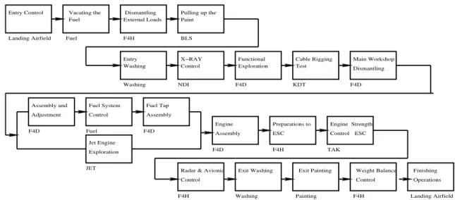
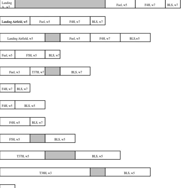
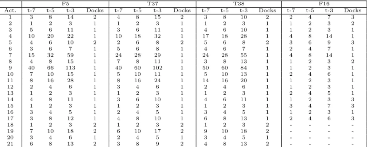
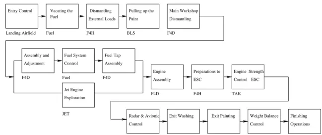
A task plan exists for FLPM where the order of the operations, the time, and the resources required to perform each operation are gathered in. This plan includes operations such as removal of all parts of the aircraft configuration, maintenance and repair of these items, and affixing the functioning parts to the aircraft so that the aircraft can fly without any problems. These operations in the task plans are well-known and fixed. In addition, different FLPM task plans are used for each aircraft configuration. Table 3.1 gives the task plan of the FLPM of F4. A row in Figure 3.1 can be read as: The activity 1 of a F4 during FLPM is in the shelter Landing Airfield and a F4 covers 3 docks space in this shelter. This activity is performed in 8 half days if a worker of skill level 7 does, 10 half days if a worker of skill level 5 does, 12 half days if a worker of skill level 3 does. Fortunately, the operation flow logic used in FLPM of all aircraft configura-tions is the same (e.g. the aircraft has to be washed before painting process)
Oper. No Oper. Name Shelter t-7 t-5 t-3 # of Docks
1 FLPM entry control Landing Airfield 8 10 12 3
2 Vacating the fuel Fuel 1 2 3 2
3 Dismantling the external loads F4H 3 6 8 1
4 Pulling up the paint BLS 16 22 28 1
5 Entry washing Washing 4 6 9 3
6 X-RAY control NDI 2 6 7 2
7 Functional exploration F4D 20 38 42 1
8 Cable rigging test KDT 9 10 18 1
9 Main workshop dismantling F4D 50 80 109 1
10 Main workshop assembly and adjustment F4D 11 12 22 1
11 Jet engine exploration JET 10 20 21 1
12 Fuel system control Fuel 3 4 6 2
13 Fuel tap assembly F4D 2 4 7 1
14 Engine assembly F4D 4 8 10 1
15 Preparations to engine strength control F4H 1 2 3 1
16 Engine strength control TAK 2 4 5 1
17 Radar and avionic system control F4H 7 10 18 1
18 Exit washing Washing 1 2 3 3
19 Exit painting Painting 5 12 18 3
20 Weight balance control F4H 3 4 5 1
21 FLPM lasting operations Landing Airfield 3 8 9 3
Table 3.1: The task plan of the FLPM of a F4
since the nature of the maintenance is similar. Therefore, the operations are called with the same names and the order of them are same; but the place they are performed and the workers used are different in these plans.
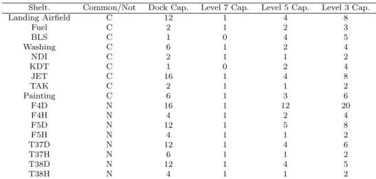
The place, where the operation is performed, is called a shelter. Some of the shelters are peculiar to the aircraft configurations which we call as PAC and some of them are used by all aircraft configurations which we call as common. Because the operation flow logic used in FLPM of all aircraft configurations is the same as mentioned before, the order of the operations performed in the common shelters are same in all precedence diagrams. There are eight PAC shelters that are F4H, F4D, F5H, F5D, T37H, T37D, T38H, and T38D. Their names imply to which aircraft configuration they are peculiar. As it is noticed, there is no shelter specialized to aircraft configuration F16. Instead, the shelters F4D and F4H are used for the operations during the FLPM of F16. Some of the shelters are common and are used during some time of FLPM of each aircraft configuration which are Fuel, BLS, Washing, NDI, KDT, JET, TAK, and Painting. As an instance, the precedence diagram of the FLPM of a F4 aircraft with the shelter,
in which the operation is performed, is given in Figure 3.1.
Entry Control Vacating the Fuel Dismantling External Loads Pulling up the Paint Entry Washing X−RAY Control Functional Exploration NDI Cable Rigging Test Main Workshop Adjustment Assembly and Dismantling Jet Engine Exploration Fuel System Control Assembly Fuel Tap Assembly Engine ESC Control Exit Washing Control
Exit Painting Weight Balance Finishing Operations Fuel F4D
F4D KDT F4D
F4D
F4H Washing Painting F4H Landing Airfield F4D F4H Preparations to ESC Engine Strength Control TAK JET Radar & Avionic
Washing
BLS F4H
Fuel Landing Airfield
Figure 3.1: Precedence diagram of a F4 aircraft
The number of docks determines the capacity of a shelter. Meanwhile, the docks are the sledges to which the aircrafts are fastened during the operations. Because the size of different aircraft configurations varies, the number of docks that they occupy is another point of consideration. For instance, F16 is a huge aircraft therefore it covers 2 docks in the shelter Fuel whereas the other aircraft configurations cover 1 dock in the same shelter. In addition, in each shelter the number of docks is known and constant. It is important to note that, the landing airfield is also represented as a shelter in our model since two operations are performed in this shelter for all aircraft configurations. Although there are no docks in the landing airfield, the space it covers is limited, which can hold 4 F4s or 6 F5s or 6 T37s or 6 T38s or 4 F16s simultaneously. In our model, we assume that the shelter landing airfield has 12 docks and the aircraft configurations F4, F5, T37, T38, F16 occupy 3, 2, 2, 2, and 3 docks respectively.
Another limited resource required to perform the operations is the workers. The operations are done by the workers who are certified by skill levels 3, 5, and 7, such that the worker of skill level 7 does operation faster than the one of skill level 5 and so on. Meanwhile, the time units that are required to perform the operations by all these 3 worker skill levels are known and given. The labor cost
of the workers is constant and increases as the skill level increases as expected. In the model, we call each skill level as a mode which are discrete. The number of workers of all three skill levels are known and constant and since they are certified to the specific operations done in each shelter, worker exchange is not possible between the shelters. Since the F4H and F4D shelters are used by both F4s and F16s, the workers in these shelters are certified to perform both the F4 and F16 specific operations which is also true for all the common shelters.
To model the FLPM exactly, the work load due to the aircrafts, which are currently in FLPM, is also taken into account. Because of this consideration, the solution procedure we propose can be applied to the problems in steady state.
Having noted a general view of the FLPM, now comes the work flow in TUAF. At the beginning of each year, the TUAF Commandership asks for the aircrafts which has FLPM due in that year from the fleets. The fleets prepare a list of those aircrafts which also includes release and due dates of FLPM for each aircraft. The arrival date of an aircraft to the Military Supply Point (MSP) for FLPM is named as release date and is known with certainty. The due date is calculated by the sum of the release date with the total processing time of FLPM assuming there are no resource constraints and a worker of level 5 is assigned to all operations. As it is noticed, the due dates set by TUAF are very tight. The TUAF Commandership sends these lists to the MSP in Eski¸sehir and asks for the cost, which consists of only the labor cost, to complete all the FLPMs of the aircrafts in the lists. In fact, the MSP determines the number of working hours required to perform the FLPMs of the aircrafts in the lists. After having the information of cost required, the TUAF Commandership could ask for a rescheduled FLPM list for a subset of the aircrafts in the initial schedule list. The MSP again calculates the incurred cost. This cycle between the commandership and the MSP is carried out till MSP ends up with a cost that can be accepted by the commandership. The reason behind this cycle is that it is not easy to find an optimal schedule, in fact even finding a feasible one under the resource and the cost constraints is not easy. In addition, the fleets and the MSP in Eski¸sehir have conflicting objectives. The fleets aim at maximizing the percentage of available aircrafts,
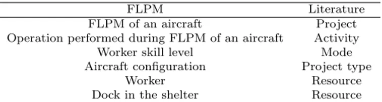
FLPM Literature
FLPM of an aircraft Project
Operation performed during FLPM of an aircraft Activity
Worker skill level Mode
Aircraft configuration Project type
Worker Resource
Dock in the shelter Resource
Table 3.2: The specific terms used in the FLPM problem and their equivalents in the literature
whereas MSP in Eski¸sehir aims at maximizing the capacity utilization. Therefore, the primary objective of the Military Supply Point is to schedule the FLPMs of the aircrafts such that the number of available aircrafts at some time instant is maximized. In order to transform this objective into scheduling terminology, the total tardiness is used as a surrogate measure. Because, the deviations from the due dates result with an increase in the number of tardy FLPMs of the aircrafts as well as a decrease in the number of available aircrafts. So by minimizing these deviations, that is minimizing the total tardiness, we can estimate the number of available aircrafts more accurately. In fact, because a ranking is made between the aircraft configurations from the availability point of view, the total weighted tardiness is to be minimized. The secondary objective of TUAF is to minimize the cost incurred for achieving this feasible schedule. However, the total weighted tardiness has much higher priority than the total incurred cost.
The described problem is an example of NRCMPSMS. The Table 3.2 shows the appropriate representations in the literature of the terms used in the FLPM problem.
After having the problem described, to develop the mathematical model of the problem, the assumptions are stated and the variables and the parameters are defined in the next section.
3.2
Preliminaries and Problem Definition
In this section, we give a formal definition of our problem described in the previous section which is the FLPM of aircrafts belonging to TUAF. The variables and the parameters used here are the ones used in the study conducted by Ahn, Erenguc and Conway in which there is only one project to be scheduled and crashability is available with the objective of minimal cost ([1], [2]). As explained in the previous section, the existence of multiple aircraft configurations differing in the precedence diagram followed and the importance weights are the additional properties of FLPM problem that are not considered in the RCMPSMS in the literature.
Throughout this work explained in this chapter, we study a deterministic project scheduling problem where all the parameters that define a problem instance are known with certainty in advance. In other words, the projects to be scheduled are known with all of their properties a priori with certainty which are the project type, the release date, the due date, and the weight. Here, the activities and the activity flows depend on the project type of the project to be scheduled, and thus project type is an important input.
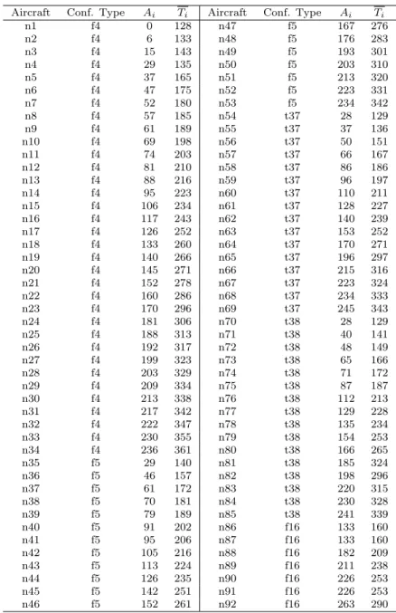
We first state the assumptions and then define the variables and the parameters necessary to formulate the FLPM problem. We are to schedule I projects of arrivals Ai of different weights wi. Each of the coming projects consists of activities to be performed are denoted by j and a project consists of J activities. Two dummy activities, 1 and J + 1 are introduced to denote the start and the completion of the projects. These activities do not require any time for processing. There are precedence relations between some activities due to technological requirements. No preemption is allowed; once an activity is started, it cannot be interrupted. The notation follows the activity-on-node format. A succeeding node gets a higher number than all of its preceding nodes. The arrivals of the projects occur at the beginning of the periods. It is important to notice that the project with a higher arrival time gets a higher number than all of its preceding projects. Sji, 1 ≤ j, denotes set of immediate successors of
the activity j of project i. Each activity j of project i can be executed in one mode available from the mode set {1, 2,. . . , Mji}. Each mode of activity j of the project i corresponds to one duration value which is dji. Meanwhile, the duration values obtained by mode selection are discrete.
For the completion of the projects, we assume that K types of renewable resources, which make mode selection available, and D types of renewable resources, which has no alternatives, are required. The D types of resources has no relation with the modes. Rk, k = 1, 2,. . . , K, units available in each period for the former resource class and Pd, d = 1, 2,. . . , D, units available in each period for the latter resource class. Again, rjmjik denotes the per period
usage of resource k, k = 1,2,. . . , K required to perform activity j of the project
i in mode mji for the former class and pjid denotes of resource d, d = 1, 2,. . . ,
D required to perform activity j of the project i for the latter. Considering the
indices, there is an index showing the dependency of the resource to the mode,
mji, where there is no such an index in the latter notation. In addition, a resource can be used by an activity of all projects in some point of the corresponding flow and a resource can be required more than once by different activities of a project type. Meanwhile, each project is assumed to have a predetermined due date,
Ti > 0.
A schedule for this problem definition consists of the finish time and mode couples for each of the J activities of all projects. A schedule is said to be feasible if:
• each activity j of each project i is assigned a mode mji ∈ {1, . . . , Mji}
• all the precedence relations are satisfied
• resource requirements in each period do not exceed their respective
capacities.
The objective of this problem is to find a feasible schedule that minimizes the total weighted tardiness. For the formulation of the problem, we introduce two additional variables which are fji and zi. fji denotes the completion time of
the activity j of the project i, j = 1,2, . . . , J; i = 1,2,. . . , I. Finish time for the activity j of a specific project i equals to the release time for the succeeding activities of the same project, Sji, namely fji = avi, v ∈Sji. Accordingly, fJi denotes the completion time of the project i. zi denotes the tardiness of the project i, and is computed as max{0, fJi− Ti} where Ti is the due date of project
i.
In the next section, the mathematical model is given according to the definition described in this section.
3.3
Modelling the Problem
Now, consider the problem defined in the previous section, NRCPSMS where the activity flow is dependent on the type of the project and the projects have different weights. The variables and the parameters used here are the ones used in the study conducted by Ahn, Erenguc and Conway in which there is only one project to be scheduled and crashability is available with the objective of minimal cost ([1], [2]). For the objective, minimum total weighted tardiness, the model can be constructed as follows:
min I X i=1 wi· zi (1) st M jiX mji=1 xjimji = 1 ∀j, i (2) fli ≤ fji− dji l = 1, 2 . . . , J − 1, j ∈ Sli, ∀i (3) f1i= 0, ∀i (4) I X i=1 X j∈SAti Mji X mji=1
rjmjik· xjimji ≤ Rk, ∀k, t = min(aji), . . . , max(fJi) (5)
I X i=1
X j∈SAti
pjid≤ Pd, ∀d, t = min(aji), . . . , max(fJi) (6)
zi ≥ fJi− Ti, ∀i (7) zi ≥ 0, ∀i (8) d1i, dJi = 0, ∀i (9) xjimji ∈ {0, 1} ∀j, i, mji (10) where Decision Variables: xjimji =
1, if activity j of project i is executed using mode mji 0, otherwise
mji = mode of the activity j of project i, ∈M(j, i) dji = duration variable of the activity j of project i
fji = finish time of the activity j of project i
SAti= the set of activities of project i that are in progress in period t; SAti =
{j : fji− dji < t ≤ fji}
zi = tardiness of project i; Z = max{0, fJi-Ti} Parameters:
Mji = the number of modes available to the activity j of project i
M(j, i) = {1, 2,. . . ,Mji) the available mode set of the activity j of project i
Ai = arrival time of the project i