Replicated partitioning for undirected hypergraphs

(1)

Contents lists available atSciVerse ScienceDirect

J. Parallel Distrib. Comput.

journal homepage:www.elsevier.com/locate/jpdc

Replicated partitioning for undirected hypergraphs

✩

R. Oguz Selvitopi,

Ata Turk,

Cevdet Aykanat

∗

Department of Computer Engineering, Bilkent University, 06800 Ankara, Turkey

a r t i c l e i n f o Article history:

Received 23 February 2011 Received in revised form 27 September 2011 Accepted 12 January 2012 Available online 23 January 2012 Keywords:

Hypergraph partitioning Recursive bipartitioning Undirected hypergraphs Replication

Iterative improvement heuristic

a b s t r a c t

Hypergraph partitioning (HP) and replication are diverse but powerful tools that are traditionally applied separately to minimize the costs of parallel and sequential systems that access related data or process related tasks. When combined together, these two techniques have the potential of achieving significant improvements in performance of many applications. In this study, we provide an approach involving a tool that simultaneously performs replication and partitioning of the vertices of an undirected hypergraph whose vertices represent data and nets represent task dependencies among these data. In this approach, we propose an iterative-improvement-based replicated bipartitioning heuristic, which is capable of move, replication, and unreplication of vertices. In order to utilize our replicated bipartitioning heuristic in a recursive bipartitioning framework, we also propose appropriate cut-net removal, cut-net splitting, and pin selection algorithms to correctly encapsulate the two most commonly used cutsize metrics. We embed our replicated bipartitioning scheme into the state-of-the-art multilevel HP tool PaToH to provide an effective and efficient replicated HP tool, rpPaToH. The performance of the techniques proposed and the tools developed is tested over the undirected hypergraphs that model the communication costs of parallel query processing in information retrieval systems. Our experimental analysis indicates that the proposed technique provides significant improvements in the quality of the partitions, especially under low replication ratios.

1. Introduction

Models and methods based on hypergraph partitioning (HP) have been successfully used for different objectives in a wide range of areas such as parallel scientific computing [4,11,15,44], very large scale integration (VLSI) circuit layout design [1,32], parallel

information retrieval (IR) [8], parallel volume rendering [9], and

database systems [12,13,40].

A hypergraph is a generalization of a graph where hyperedges (nets) connect one or more vertices (cells). The HP problem is defined as the task of dividing the vertex set of a given hypergraph into disjoint subsets such that the cost (cutsize) is minimized while a certain balance constraint on the part weights is satisfied. The cutsize is generally a function of the nets that connect more than one part.

Hypergraphs can be used to represent different types of relation in a wide range of problems which can broadly be categorized into two as directed and undirected relations. Depending on

✩ _{This work is partially supported by the Scientific and Technological Research}

Council of Turkey (TÜBİTAK) under project EEEAG-109E019.

∗_{Corresponding author.}

E-mail addresses:reha@cs.bilkent.edu.tr(R. Oguz Selvitopi), atat@cs.bilkent.edu.tr(A. Turk),aykanat@cs.bilkent.edu.tr(C. Aykanat).

the category of the relation, directed or undirected hypergraphs are used in the modeling. In undirected hypergraphs, a net is used to model an equally shared relation among the tasks/data represented by the vertices it connects. In directed hypergraphs, a net is used to model an input–output relation among the tasks/data represented by the vertices it connects.

We use the terms directional and undirectional HP models for indicating models based on partitioning of directed and undirected hypergraphs, respectively. We should note here that almost all of the state-of-the-art HP tools [2,14,26,43,45] are designed to partition undirected hypergraphs. Hence, some special techniques

such as consistency condition [11] and the elementary hypergraph

model [44] are utilized to model some types of directed relations

correctly via undirectional HP models.

The schemes that combine vertex replication with HP models have only been studied for directional HP models in the context of VLSI circuit layout design. In these HP models, since the vertices generally model the gates or logic devices, replication corresponds to duplicating the same gate or logic device in multiple networks of a partitioned logic network. In this way, the number of connections between networks and the wiring density can be reduced at the expense of implementing the same logic in multiple networks.

In directional HP models, vertex replication may cause an increase in the cutsize, and it generally requires further replication of other vertices and nets. However, in undirectional HP models,

(2)

since an input–output relation does not exist between the vertices connected by a net, replication does not have such an effect. This forms the basic difference between vertex replication in directional and undirectional HP models. To the best of our knowledge, there are no studies in the literature addressing vertex replication schemes for undirectional HP models. In this study, we try to fill this gap. Note that, due to the above-mentioned fundamental difference in vertex replication, the techniques we present here are not directly applicable to directional HP models. Thus, replication in undirectional HP models requires specific techniques and tools tailored for this purpose.

1.1. Related work in directional HP models

Even though we do not address applications in the VLSI domain, we discuss replication schemes in this area, since, to our knowl-edge, VLSI circuit layout design is the only area where HP is ap-plied together with replication, albeit in a directional partitioning framework.

Replication schemes in VLSI circuit layout design and partition-ing arise in the form of gate replication to reduce pin counts and the interconnection cost of the partitioned circuits. These schemes can be categorized into two as one-phase schemes and two-phase schemes with respect to when the partitioning and replication are performed. In the one-phase approach, partitioning and replica-tion are performed simultaneously, whereas in the two-phase ap-proach replication is performed after obtaining a partition. In the one-phase approach, generally, extended versions of the Fiduc-cia–Mattheyses (FM) [17] heuristic are utilized [30,31]. In the two-phase approach, after obtaining a partition, linear programming

or flow-network [22,33] formulations are used to achieve

repli-cation, and often, if needed, an extended FM heuristic is applied as the last step to find a feasible solution. Since this study fo-cuses on performing replication and partitioning simultaneously, we briefly summarize the existing work on FM heuristics for

di-rectional graph/hypergraph partitioning with replication. In [30],

an extended version of the FM algorithm for directional HP mod-els is proposed to perform replication in two-way partitioned net-works by introducing new definitions for cell/net states and cell

gains. The authors of [31] introduce an extended version of the FM

algorithm to achieve partitioning and replication, and they propose a new gain definition and objective function for this extended

ver-sion. In [33], the authors use a modified FM algorithm applied over

a replication graph which they obtain by a linear programming formulation. A detailed discussion and comparison of replication

techniques in circuit partitioning can be found in [16].

1.2. Application

In order to show the validity of the algorithms proposed in our paper, we investigate undirectional HP models proposed for

index partitioning of parallel IR systems [8,28], where replication

is beneficial and commonly used [37]. Although we address the HP

models used in parallel IR, our replication scheme can be used for any domain in which the underlying problem can be modeled as an undirected hypergraph.

In parallel IR systems, the index is partitioned across several machines [7,23,36,38,41], typically in a document-based or term-based fashion, in order to process very large text collections. In [42], it is remarked that replication is necessary for improving query

throughput. The authors of [35] propose a bin-packing-based

greedy algorithm that utilizes query logs to distribute terms to index servers. In their experiments, they replicate a small amount of most frequent terms and discover that replication is a powerful tool in reducing the average number of per-query servers, even under low replication ratios. In the distributed IR system of Google,

the entire system is replicated [5]. A selective replication scheme

that replicates inverted lists of high workload terms to improve load balancing in a pipelined and term-distributed IR system is investigated in [37].

In the HP models utilized for term-based distribution of

inverted indices [28], the vertex

v

irepresents the term tiand the

task of retrieving its inverted list. The net njrepresents the query

qjand connects the subsets of vertices that represent the terms

requested by that query. In this HP model, the nets have unit costs

due to the infinite result cache capacity assumption.1_{The weight of}

a vertex is set equal to either the number of postings in the inverted

list of the term represented by that vertex [8] or the multiplication

of term popularity and the corresponding posting list size [37].

The balance constraint in the former vertex weighting scheme corresponds to maintaining storage balance, whereas the balance constraint in the latter vertex weighting scheme corresponds to maintaining computational workload balance. The partitioning objective of minimizing the cutsize corresponds to minimizing the communication volume during parallel query processing.

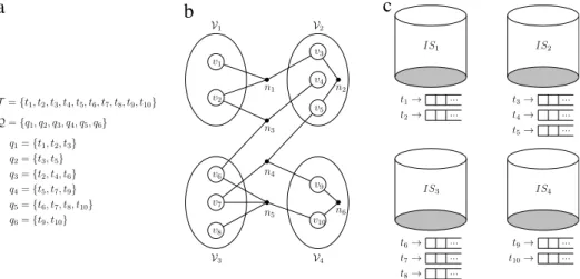
We introduceFig. 1to illustrate the relationship between the

target application and undirectional HP models.Fig. 1(a) shows

a sample term collection T that contains ten terms together

with a query logQthat contains six queries.Fig. 1(b) shows the

undirectional hypergraph model for this sample inverted index. As seen inFig. 1(b), net n1connects vertices

v

1

, v

2, and

v

3, since query

q1requests the terms t1

,

t2, and t3.Fig. 1(b) also shows a four-way

partition of this hypergraph.Fig. 1(c) shows the distribution of the

sample inverted index among four index servers (IS1

, . . . ,

IS4) that is induced by this four-way partition. For example, the index server

IS2stores the terms t3

,

t4, and t5and their inverted lists since part V2of the partition consists of the vertices

v

3

, v

4, and

v

5.

The correspondence between vertex replication and the men-tioned HP model is as follows. A net in this HP model represents the undirectional shared relation among the respective retrieval tasks that can be performed concurrently and independently on the inverted lists represented by the vertices connected by that net. Thus, vertex replication corresponds to replicating inverted lists of terms for further minimization of the communication volume. For a given query, the task associated with each data is only performed by one of the processors owning the replicas of that data. Thus, the proposed scheme incurs redundant storage (data replication) but does not incur redundant computation.

1.3. Contributions

There are five main contributions of this study. (1) The dif-ferences between vertex replication in directional and

undirec-tional HP models are explained (Section3). (2) A vertex replication

scheme for undirectional HP models is proposed (Section 4).

This replication approach is based on an iterative-improvement heuristic, and it achieves replication during partitioning. For this purpose, the FM heuristic is extended to support replication and unreplication of vertices in addition to vertex moves. This extended heuristic is called rFM, and it operates on a given two-way partition (bipartition) by introducing new gain definitions and vertex states. (3) In order to utilize rFM in a recursive bipartitioning (RB) frame-work, appropriate cut-net removal, cut-net splitting, and pin selec-tion algorithms are proposed to correctly encapsulate the two most

commonly used cutsize metrics (Sections5and6). (4) The

pro-posed vertex replication and bipartitioning scheme is integrated

into the state-of-the-art multilevel HP tool

PaToH

[2] that uses

1 This assumption simply states that each query is processed only once and its results are stored in the result cache. Further requests for the same query are responded from this result cache [10].

(3)

a

_b

c

Fig. 1. The relation between an inverted index distribution and undirectional HP models. (a) A sample inverted index, (b) the corresponding hypergraph model, and (c) a

four-way term-based inverted index distribution.

the RB paradigm to provide a replicated HP tool,

rpPaToH

.

Specifi-cally, the uncoarsening phase of the multilevel framework is mod-ified by using rFM as a replicated partitioning and refinement tool. At each level of the uncoarsening phase, the rFM algorithm is run and the multilevel scheme is extended to support replicated ver-tices. (5) Detailed experimental analyses are performed over the

hypergraph model of the sample application (Section1.2) using

synthetic and realistic datasets. The results obtained indicate that

rpPaToH

performs significantly better than a successful

partition-ing and replication scheme [28] for this application domain.

The rest of the paper is organized as follows. Section2gives the

necessary background. Section3explains the differences between

replication in directional and undirectional HP models. Section4

describes the details of the rFM heuristic. Section 5 presents

the proposed cut-net removal, cut-net splitting, and replication

distribution schemes. Section6addresses the pin selection issue

after obtaining a K -way partition. Section7discusses the results of

the experiments that were carried out. Finally, Section8concludes.

2. Background and problem definition

2.1. Definitions and hypergraph partitioning problem

A hypergraphH

=

(

V

,

N

)

is defined as a set of verticesVand

a set of netsN. Each net nj

∈

N connects a subset of vertices.

The set of vertices connected by net njis denoted as Vertices

(

nj

)

.

The set of nets that connect vertex

v

iis denoted as Nets

(v

i

)

. The

vertices

v

iand

v

jare said to be neighbors if they are connected by

at least one common net, i.e., Nets

(v

i

) ∩

Nets

(v

j

) ̸= ∅

. An

(

nj

, v

i

)

tuple denotes a pin of njwhere

v

i

∈

Vertices

(

nj

)

. The degree of a net njis equal to the number of vertices it connects,

|

Vertices

(

nj

)|

.

The total number of pins P

=



nj∈N

|

Vertices

(

nj

)|

denotes the

size of a given hypergraphH. A weight value

w(v

i

)

is associated

with each vertex

v

i, and a cost value c

(

nj

)

is associated with each

net nj. The cost function for a net easily extends to a subset of nets

M

⊆

N, i.e., c

(

M

) = 

_nj∈Mc

(

nj

)

.

Π

= {

V1

, . . . ,

VK

}

is a K -way partition ofH

=

(

V

,

N

)

if each

partVkis a nonempty subset ofV, the parts are pairwise disjoint,

and the union of K parts is equal toV. The weight W

(

Vk

)

of a

partVkis the sum of the weights of the vertices in that part, i.e.,

W

(V

k

) = 

_v_i∈Vk

w(v

i

)

. A partitionΠis said to be balanced if each

partVk

∈

Πsatisfies the balance constraint:

W

(

Vk

) ≤ (

1

+

ϵ)

Wavg for k

=

1

, . . . ,

K

,

(1)

where Wavg

=

W

(

V

)/

K and

ϵ

is the predetermined maximum

imbalance ratio.

In a partitionΠ, a net is said to connect a part if it connects at

least one vertex in that part. The connectivity setΛ(nj

)

of a net njis

defined as the set of parts connected by nj. The number of parts in

the connectivity set of njis denoted by

λ(

nj

) = |Λ(

nj

)|

. A net is said to be cut or external if it connects more than one part (

λ(

nj

) >

1), and uncut or internal if it connects only one part (

λ(

nj

) =

1). The set of external nets in a partitionΠis denoted asNE. The set of internal

nets that connect a vertex

v

iis denoted as InternalNets

(v

i

)

. Two

cutsize metrics widely used in the literature to represent the cost

of a partitionΠare cutsize

(Π

) =



nj∈NE c

(

nj

),

(2) cutsize

(Π

) =



nj∈NE

(λ(

nj

) −

1

)

c

(

nj

).

(3)

The cost definitions in Eqs.(2)and(3)are called the cut-net metric

and the connectivity metric, respectively. For example, the cut-net and connectivity metrics model the minimization of the commu-nication volume in parallel sparse matrix vector multiplication utilizing collective and point-to-point communication schemes, respectively [11,44].

Given a hypergraph H

=

(

V

,

N

)

, hypergraph partitioning

can be defined as finding a K -way partitionΠ

= {

V1

, . . . ,

VK

}

that minimizes the cutsize (Eqs. (2) or (3)) while maintaining

the balance constraint (Eq. (1)). This problem is known to be

NP-hard [32].

2.2. Iterative improvement heuristics for two-way HP

FM-based schemes [1,17] are widely used

iterative-improve-ment heuristics to solve the HP problem. FM-based heuristics improve the cutsize of a bipartition by moving vertices from one part to the other. The gain of a vertex in these heuristics is generally defined as the reduction in the cutsize if that vertex were to be moved to its complementary part in a bipartition. FM heuristics can perform multiple passes over all vertices until the improvement in the cutsize drops below a certain threshold.

2.3. Recursive bipartitioning and multilevel frameworks

RB is the most commonly used method for obtaining a K -way partition of a hypergraph, although there are other methods based

on direct K -way partitioning [3,27]. In the RB scheme, first a

(4)

bipartition is decoded to construct two subhypergraphs using the

cut-net removal and cut-net splitting techniques [2] to capture

the cut-net and connectivity cutsize metrics, respectively. Then these two subhypergraphs are further bipartitioned in a recursive manner. This procedure continues until desired number of parts is reached (in log K recursion levels for K parts).

FM-based heuristics perform poorly on hypergraphs with high

net degrees [3,27] and small vertex degrees [19]. To alleviate

these problems, multilevel algorithms have been proposed [6,20]

and applied to the HP problem, leading to successful HP tools

such as

PaToH

[2], hMeTiS [26], Mondriaan [45], Zoltan [14], and

ParKWay [43].

Multilevel methodology consists of coarsening, initial partition-ing, and uncoarsening phases. In the coarsening phase, the original hypergraph is coarsened into a smaller hypergraph by a sequence of coarsening levels, where, in each level, various matching and clustering algorithms are used to form super-vertices from highly coherent vertices. Coherent vertices are the vertices that share high number of nets. In the initial partitioning phase, a bipartition of the coarsest hypergraph is obtained, and this coarsest hypergraph is projected back to the original hypergraph in the uncoarsen-ing phase. At each level of the uncoarsenuncoarsen-ing phase, FM-based or

KL-based [29] refinement heuristics are used to improve the

quality of the bipartitions.

3. Replication in directional versus undirectional HP models

There are two main differences between vertex replication in directional and undirectional HP models. (i) The replication of a vertex in directional HP models may bring internal nets to the cut and thus can increase the cutsize of a partition, and (ii) vertex replication generally requires further net and pin replication in directional HP models. However, these two cases are not valid for undirectional HP models.

In directed hypergraphs, the nets that connect a vertex

v

i are

categorized as input and output nets of

v

i. In a dual manner,

the vertices that are connected by a net nj are categorized as

input and output vertices of nj. For example, in hypergraph

representation of gate-level VLSI circuits for layout design [1]

and column-net hypergraph representation of sparse matrices for

parallel matrix–vector multiplication [11], nets have single input

and multiple output vertices, which correspond to vertices having multiple input and single output nets.

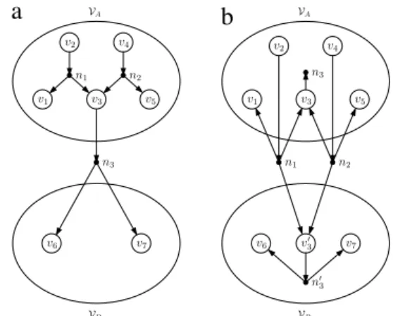
In directional HP models, when an output vertex

v

i of an

internal net njis replicated, njbecomes cut since any new instance

of the replicated vertex

v

′

i must be fed by nj on the part it

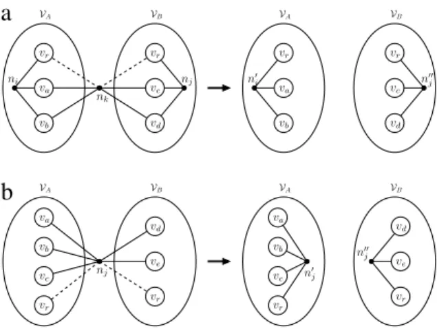
is replicated to. Fig. 2 shows an example of vertex replication

in a directed hypergraph. A sample bipartition on this directed

hypergraph is illustrated inFig. 2(a). Initially, the cutsize of the

bipartition is one, assuming that the nets have unit costs. As shown inFig. 2(b), when

v

3is replicated, n1and n2become cut since

v

3

is an output vertex of these internal nets. Since

v

′

3has to be fed

by both of these nets, pins

(

n1

, v

3′

)

and

(

n2

, v

′3

)

are generated in

Fig. 2(b). Furthermore, when an external net nj’s input vertex

v

iis

replicated, njis generally replicated together with

v

ito be able to

save njfrom the cut. As shown inFig. 2(b), when

v

3is replicated, n3

is also replicated, leading to the addition of a new net n′₃and a new

(

n′ 3

, v

′

3

)

inVB. In this way, we are able to save n3from the cut.

However, since n1and n2become cut, the cutsize of the bipartition

increases from one to two after the replication.

In contrast, in undirectional HP models, performing replication does not bring internal nets to the cut, and putting additional pins to the new instances of the replicated vertices may not be necessary, since a net represents a shared relation rather than a dependence among the vertices it connects. In other words, we can make a choice among the instances of a replicated vertex for a

a

_b

Fig. 2. Replication in a directed hypergraph. (a) Initial bipartition, (b) after replicatingv3.

a

_b

Fig. 3. Replication in an undirected hypergraph. (a) Initial bipartition, (b) after

replicatingv3.

net in order to decide which one of these instances will represent that replicated vertex. This is done by putting a pin only to a

single instance of the replicated vertex for that net.Fig. 3shows

an example of vertex replication in an undirected hypergraph.

The initial bipartition is seen inFig. 3(a), which is the undirected

version of the directed hypergraph inFig. 2(a) and has a cutsize of

one. As opposed to replication of

v

3inFig. 2, replication of

v

3in

Fig. 3does not bring any internal net to the cut, since, as seen in

Fig. 3(b), the nets n1and n2are not required to feed

v

3′. Instead, n1 (or similarly n2and n3) can ‘‘choose’’ to use either

v

3or

v

′3, since n1 just needs to select an instance for this replicated vertex. In other

words, n1has to have just one pin to an instance of the replicated

vertex, which is selected to be the pin

(

n1

, v

3

)

in this example. We refer to this problem as the pin selection problem and address it

in Section6. After replication of

v

3, the cutsize of the bipartition

reduces from one to zero.

Having described the differences between vertex replication in directional and undirectional HP models, we set our focus on replication in undirectional HP models and define the Replicated

Undirected Hypergraph Partitioning problem as follows: given an

undirected hypergraphH

=

(

V

,

N

)

, an imbalance ratio

ϵ

, and

a replication ratio

ρ

, find a K -way covering subset ofV

,

ΠR

₌

{

V1

, . . . ,

VK

}

that minimizes the cutsize (Eqs. (2) or (3)) while satisfying the following constraints.

•

Balancing constraint: Wmax

≤

(

1

+

ϵ)

Wavg, where

Wmax

=

max

1≤k≤KW

(

Vk

)

and Wavg

=

(

1

+

ρ)

W

(

V

)/

K

.

•

Replication constraint:



K

(5)

a

_b

c

Fig. 4. Move and replication of a vertex. (b) Initial bipartition, (a) after movingv1fromVAtoVB, and (c) after replicatingv1fromVAtoVB.

Note that Wmaxdenotes the weight of the maximally weighted part,

Wavg denotes the part weight under perfect balance, and W

(

V

)

denotes the total vertex weight without replication.

4. Replicated FM (rFM)

We propose an extended FM heuristic which we call replicated

FM (rFM) to address the Replicated Undirected Hypergraph Partition-ing problem.

4.1. Definitions

In a two-way covering subsetΠR

_{= {}

_V

A

,

VB

}

ofV, a vertex can belong toVA

,

VB, or both of them if it is replicated, and hence it can be in one of three states, A

,

B, and AB:

State

(v

i

) =



_A _if

v

i

∈

VAand

v

i

̸∈

VB

,

B if

v

i

∈

VBand

v

i

̸∈

VA

,

AB if

v

i

∈

VAand

v

i

∈

VB

.

Herein, a covering subsetΠR_of_V_{will be referred to as a replicated}

partition ofV, and subsets ofΠRwill be referred to as parts ofΠR. Each instance of a replicated vertex is referred to as a replica. The

number of non-replicated vertices in state A and connected by njis

denoted as

σ

A

(

nj

)

. The number of non-replicated vertices in state B and connected by njis denoted as

σ

B

(

nj

)

. Similarly, the number of replicated vertices (not the number of replicas) that are connected by njis denoted as

σ

AB

(

nj

)

. Note that, according to the definitions,

|

Vertices

(

nj

)| = σ

A

(

nj

) + σ

B

(

nj

) + σ

AB

(

nj

).

A net njin a two-way replicated partition is said to be cut if both

σ

A

(

nj

) >

0 and

σ

B

(

nj

) >

0. The cut-state of a net is used to describe whether that net is cut or not. A net njis said to be internal toVAif

σ

B

(

nj

) =

0 and it is said to be internal toVBif

σ

A

(

nj

) =

0. A net nj can be considered internal to eitherVAorVBif

σ

A

(

nj

) =

0

, σ

B

(

nj

) =

0 and

σ

AB

(

nj

) >

0.

rFM is an iterative-improvement heuristic that tries to improve the cutsize of a given two-way replicated partition by move, replication, and unreplication operations performed on vertices. The move and replication operations can only be performed on non-replicated vertices, whereas the unreplication operation can only be performed on replicated vertices. A non-replicated vertex has two gains, which are move and replication gains. Similarly, a replicated vertex also has two gains, which are unreplication from

VAand unreplication fromVB gains. The gain definitions are as

follows.

•

The move gain, gm

(v

i

)

, of a non-replicated vertex

v

iis defined as

the reduction in the cutsize if

v

iwere to be moved to the other

part. The move gain of

v

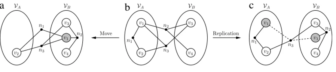
iis equal to the difference between the

sum of the costs of the nets saved from the cut and the sum of the costs of the internal nets that are brought to the cut.Fig. 4(b)

and (a) display the move of

v

1fromVAtoVB. Moving

v

1from

VAtoVBbrings net n1into the cut while saving net n2from the

cut. Hence, gm

(v

1

) =

c

(

n2

) −

c

(

n1

)

. After the move operation,

v

1is locked. The locked vertices in the examples are illustrated

by gray color.

•

The replication gain, gr

(v

i

)

, is defined as the reduction in the

cutsize if vertex

v

iwere to be replicated to the other part. The

replication gain of

v

i is equal to the sum of the costs of the

nets saved from the cut. When a vertex is replicated, it cannot bring any internal net to the cut and thus cannot increase the cutsize. This forms the basic difference between the move and

replication operations. Consequently, for any vertex

v

i, we have

gr

(v

i

) ≥

0 and gr

(v

i

) ≥

gm

(v

i

)

.Fig. 4(b) and (c) show the replication of

v

1fromVAtoVB. The replication of

v

1saves net

n2 from the cut as the move of

v

1does; however, net n1 still

remains as an internal net, as opposed to the move operation

on the same vertex. Hence, gr

(v

1

) =

c

(

n2

)

. In the examples,

if a net is internal to a part and connects a replicated vertex, we illustrate this by putting a pin to the replica that is in the part of the internal net and omit the pin to the other replica. In contrast, if an external net connects a replicated vertex, the pins to the replicas of the replicated vertex connected by that net are displayed by dashed lines.

•

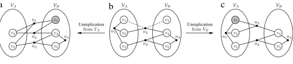
The unreplication gain, gu,A

(v

i

)

or gu,B

(v

i

)

, is defined as the

reduction in the cutsize if a replica of the replicated vertex

v

i

were to be unreplicated from its part. Since unreplication of a replica cannot improve the cutsize, the maximum unreplication

gain of a replica is zero. Thus, for any replicated vertex

v

i,

gu,A

(v

i

) ≤

0 and gu,B

(v

i

) ≤

0. A replica with an unreplication gain of zero implies that this replica is unnecessary and its removal will not change the cutsize. On the other hand, if the unreplication gain of a replica is negative, this implies that the replica is necessary and its unreplication will bring internal

net(s) to the cut.Fig. 5shows the unreplication of a necessary

and an unnecessary replica. Initially, there are two replicas of

v

1

in the bipartition inFig. 5(b). The replica inVAis necessary, and

its unreplication causes the internal net n1to be cut, as seen in

Fig. 5(a). On the other hand, the replica inVBis unnecessary, and its unreplication does not change the cut set, as seen inFig. 5(c). Hence, gu,A

(v

1

) = −

c

(

n1

)

and gu,B

(v

1

) =

0.

4.2. Overall rFM algorithm

Replicated FM performs a predetermined number of passes considered on all vertices, where each pass comprises a sequence of operations (Algorithm 1). First, we compute the two possible gains for each vertex and initialize the pin distributions of the nets (line 1). At the beginning of each pass, we unlock all vertices to be able to perform operations on them (line 3). Then the algorithm enters the inner while loop (lines 4–7). In this loop, we first select a vertex and an operation (move, replication, or unreplication) to be performed on the selected vertex (line 5) according to the operation selection criteria described below. Then we perform the selected operation if it does not violate the size constraints on the weights of the parts (line 6). After the selected operation is performed on the vertex, the selected vertex is locked and the gain values of its unlocked neighbors and the pin distributions of the nets that connect this vertex are updated (line 7). A pass terminates when there are no more valid operations. At the end of a pass, a

(6)

a

_b

c

Fig. 5. Unreplication of instances of a replicated vertex. (b) Initial bipartition, (a) after unreplicating the replica ofv1fromVA, and (c) after unreplicating the replica ofv1

fromVB.

rollback procedure is applied to the point where the bipartition with the minimum cutsize is seen (line 8).

The size constraint check performed during the operation selection is done as follows. (i) If the selected operation is a move or a replication, the new weight of the destination part if the selected

operation were to be performed is computed, and, if it exceeds

(

1

+

ϵ)

Wavg, this operation is discarded, and (ii) if the selected operation is unreplication, it is checked if the weight of the part on which

unreplication were to be performed drops below

(

1

−

ϵ)

Wavg, and,

if it does, it is discarded. Furthermore, if the selected operation is replication, it is only performed if the total amount of replication performed up to that point plus the weight of the selected vertex

does not exceed the allowed replication amount

ρ

W

(

V

)

.

Algorithm 1: Basic steps of rFM. Input:H =(V, N ), ΠR_{= {V}

A, VB}

Initialize pin distributions, gains, and priority queues.

1

while there are passes to perform do

2

Unlock all vertices.

3

while there is any valid operation do

4

(v,op) ←Select the vertex and the operation to perform on

5

it.

Perform op onv, store the reduction in the cutsize, and lock

6

v.

Update the gains of unlocked neighbors ofvand the pin

7

distributions of the nets in Nets(v).

Rollback to the point when minimum cutsize is seen.

8

Operation selection: We use a priority-based selection approach

for determining the current operation and disallow some opera-tions that do not satisfy certain condiopera-tions. The selection strategy is based on principles such as minimizing the number of unneces-sary replicas, limiting the replication amount, and improving the balance. We give the highest priority to the elimination of unnec-essary replicas. We do not perform unreplication operations with negative gains simply because such operations will degrade the cutsize. If there are no unnecessary replicas, we make a choice be-tween move and replication by selecting the operation with the higher gain. Ties between the gains of the selected move and repli-cation operations are broken in favor of the move operations. Any replication with a gain value of zero is disallowed since such oper-ations will produce unnecessary replicas. However, the zero-gain moves that improve the balance are retained. Since, for any ver-tex

v

i, gr

(v

i

) ≥

gm

(v

i

)

, in a single pass, the number of replica-tion operareplica-tions tends to outweigh the number of move operareplica-tions. This issue can be addressed by the gradient methodology, which we discuss below.

Gradient methodology: The gradient methodology is used in

FM heuristics that are capable of replication for directed graph

models [34] to obtain partitions with better cutsize. The basic

idea of the gradient methodology is to introduce the replication in the later iterations of a pass, especially when the improvement achieved in the cutsize by performing only move operations drops

below a certain threshold. As mentioned in [16], early replication

can have a negative effect on the final partition by limiting the algorithm’s ability to change the current partition. Furthermore, by using the replication in the later iterations, the algorithm can climb out of the local minima reached by the move operations. In rFM, we adopt and modify the gradient methodology by allowing only move and unreplication operations until the improvement in the cutsize drops below a certain threshold, and then we allow replication operations.

Early exit: We use the early-exit scheme [18] to improve the run-time performance of rFM. In this scheme, if there are no improvements in the cutsize for a predetermined number of successive iterations, the current pass of the FM algorithm is terminated since it is unlikely to further improve the cutsize.

Locking: In conventional move-based FM algorithms, after

moving a vertex, it is locked to avoid thrashing [17]. Similarly, in

rFM, we also lock the operated vertex after performing a move, replication, or unreplication operation on that vertex.

Data structures: We maintain six priority queues keyed

according to the gain values of the vertices with respect to type of operation. The heaps are implemented as binary heaps. For each part, we have three heaps for storing the move, replication, and unreplication gains. The two gains associated with a non-replicated vertex are stored in the move and replication heaps of the part that the vertex belongs to. Similarly, the two gains associated with the replicas of a replicated vertex have their unreplication gains stored in the unreplication heap of their respective parts.

4.3. Net criticality

The main power of rFM, like all FM-based algorithms, lies in its

efficient linear-time gain update operations [17]. In this section,

we present net criticality definitions that trigger updates on move, replication, and unreplication gains.

A net njis said to be critical to partVk, if an operation performed

on a vertex

v

i

∈

Vk can change the cut-state of nj. Whenever

an operation is performed on a vertex

v

i, we check the criticality

conditions of the nets that connect

v

i. If the criticality condition

of a net nj that connects

v

i changes, the other vertices that

are connected by njare checked for gain updates. Each type of

operation imposes different pin distributions for the criticality of nets; thus the criticality definition of a net is classified as move criticality, replication criticality, and unreplication criticality, according to the type of operation that causes a change in the cut-state of the respective net.

For a net to be move critical, it must connect at least two non-replicated vertices (

σ

A

(

nj

) + σ

B

(

nj

) >

1), and it must either be an internal net or an external net with a single pin in one of the two parts. As seen inTable 1, a net njis move critical toVAif (

σ

A

(

nj

) =

1 and

σ

B

(

nj

) >

0) or (

σ

B

(

nj

) =

0 and

σ

A

(

nj

) >

1), and toVBif (

σ

A

(

nj

) =

0 and

σ

B

(

nj

) >

1) or (

σ

B

(

nj

) =

1 and

σ

A

(

nj

) >

0).

For a net to be replication critical, it must connect at least two non-replicated vertices (

σ

A

(

nj

) + σ

B

(

nj

) >

1), and it must be an

(7)

Table 1

Criticality definitions for a net njtoVAandVB. For example, njis replication critical toVAifσA(nj) =1 andσB(nj) >0.

njis Move critical Replication critical Unreplication critical

ToVAif

(σA(nj) =1 andσB(nj) >0) σA(nj) =1 andσB(nj) >0 or

(σB(nj) =0 andσA(nj) >1) σB(nj) =0 andσA(nj) >0 andσAB(nj) >0 ToVBif

(σA(nj) =0 andσB(nj) >1) σA(nj) =0 andσB(nj) >0 andσAB(nj) >0 or

(σB(nj) =1 andσA(nj) >0) σB(nj) =1 andσA(nj) >0

external net with a single pin in one of the two parts. As seen in

Table 1, a net nj is replication critical toVA if (

σ

A

(

nj

) =

1 and

σ

B

(

nj

) >

0), and toVBif (

σ

B

(

nj

) =

1 and

σ

A

(

nj

) >

0). Note that the internal nets which are always move critical are never replication critical, since the replication of a vertex connected by an internal net cannot change the cut-state of that net. This difference

is indicated inTable 1, where the conditions (

σ

B

(

nj

) =

0 and

σ

A

(

nj

) >

1) and (

σ

A

(

nj

) =

0 and

σ

B

(

nj

) >

1), which exist in the move-critical column, do not appear in the replication-critical column.

For a net to be unreplication critical, it must be an internal net that connects at least one non-replicated and one replicated vertex (

σ

A

(

nj

) + σ

B

(

nj

) >

0 and

σ

AB

(

nj

) >

0). As seen inTable 1, a net

njis unreplication critical toVA if (

σ

B

(

nj

) =

0 and

σ

A

(

nj

) >

0 and

σ

AB

(

nj

) >

0), and to VB if (

σ

A

(

nj

) =

0 and

σ

B

(

nj

) >

0 and

σ

AB

(

nj

) >

0). Note that external nets that connect a single non-replicated vertex in only one of the two parts, which are move critical, are never unreplication critical, since unreplication of a vertex connected by an external net cannot change the

cut-state of that net. This difference is indicated inTable 1, where the

conditions (

σ

A

(

nj

) =

1 and

σ

B

(

nj

) >

0) and (

σ

B

(

nj

) =

1 and

σ

A

(

nj

) >

0), which are shown in the move-critical column do not appear in unreplication-critical column.

4.4. rFM algorithm details

In this section, we present detailed explanations of some of the non-trivial concepts and algorithms used in rFM. The examples respect the basics of the operation selection criteria mentioned in

Section4.2. For the sake of simplicity, we assume that each net

has unit cost, and we also overlook the balance constraints on part weights in the examples.

Initial gain computation. The initial gain computation, which is

performed at the beginning of each pass of rFM, is given in Algorithm 2 and consists of two main loops. The first loop resets the initial gain values by traversing vertices (lines 1–7) and the second loop completes the initialization of gains by traversing all pins (lines 8–18). The move and replication gains are computed according to the external and critical nets that connect these vertices, whereas the unreplication gains are modified according to the internal and critical nets that connect these vertices.

The move and replication gains of the non-replicated vertices are initially set to their minimum possible values (lines 3–4). If

a net nj is external and move critical or replication critical, the

move and replication gains of the vertices connected by njmust

be incremented by c

(

nj

)

(lines 12–13), since it can be saved from

the cut with either one of these operations. In contrast to move and replication gains, unreplication gains are initially set to their

maximum possible values (lines 6–7). If a net njis internal and thus

unreplication critical, the unreplication gains of the replicas of the

replicated vertices connected by njmay need to be updated. The

unreplication gains of the replicas that are in the same part with

this internal net need to be decremented by c

(

nj

)

if njconnects at

least one non-replicated vertex that is in the same part with this net (lines 14–18).

Algorithm 2: Initial move, replication, and unreplication gain

computation. Input:H =(V, N ), ΠR_{= {V} A, VB} foreachvi∈ Vdo 1 if State(vi) ̸=AB then 2 gm(vi) ← −c(InternalNets(vi)) 3 gr(vi) ←0 4 else 5 gu,A(vi) ←0 6 gu,B(vi) ←0 7 foreach nj∈ N do 8 foreachvi∈Vertices(nj)do 9

if State(vi) ̸=AB and njis external then

10

if (σA(nj) =1 and State(vi) =A) or (σB(nj) =1 and

11

State(vi) =B) then ◃njis critical toVAorVB gm(vi) ←gm(vi) +c(nj)

12

gr(vi) ←gr(vi) +c(nj)

13

else if State(vi) =AB and njis internal then

14

ifσA(nj) >0 andσB(nj) =0 then ◃njis critical toVA

15

gu,A(vi) ←gu,A(vi) −c(nj)

16

else ifσB(nj) >0 andσA(nj) =0 then ◃njis critical to

17

VB

gu,B(vi) ←gu,B(vi) −c(nj)

18

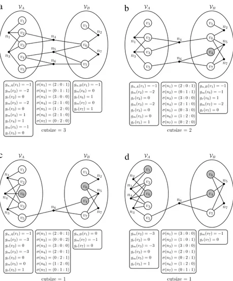
Fig. 6(a) shows the pin distributions of the nets and the gain values of the vertices for a sample bipartition after Algorithm 2 is run on this sample. Nets n4

,

n5, and n6are cut; thus the cutsize of

the bipartition inFig. 6(a) is three. We use the notation

σ (

nj

) =

(σ

A

(

nj

) : σ

B

(

nj

) : σ

AB

(

nj

))

to denote the pin distribution of nj.

Gain updates after a move operation. Algorithm 3 shows the

pro-cedure for performing gain updates after moving a given vertex

v

∗

fromVAtoVB. The algorithm includes updating fields of

v

∗(lines

1–2), the pin distributions of Nets

(v

∗

₎

_{(lines 4 and 16), and the}

gain values of neighbors of

v

∗(lines 5–15 and 17–27). The

neces-sary field updates on

v

∗are performed by updating the state and

locked fields of

v

∗_{to reflect the move operation. The pin}

distri-bution of each net nj

∈

Nets

(v

∗

)

needs to be updated by

decre-menting

σ

A

(

nj

)

by 1 and incrementing

σ

B

(

nj

)

by 1. When the pin

distribution of njchanges, its criticality may change with respect

to the operation type. The change in the criticality of njmay

re-quire various gain updates on the unlocked vertices connected by nj.

After decrementing the number of vertices of njinVA(line 4),

we check the value of

σ

A

(

nj

)

to see if the criticality of njhas changed

(lines 5 and 11). If

σ

A

(

nj

) =

0

,

nj becomes internal to VB by

becoming move critical and unreplication critical to this part, and if

σ

A

(

nj

) =

1

,

njbecomes move critical and replication critical toVA. Similarly, after incrementing the number of vertices connected by

njinVB(line 16), we check the value of

σ

B

(

nj

)

to see if the criticality of njhas changed (lines 17 and 23). If

σ

B

(

nj

) =

1, it means that nj was internal and hence was move critical and unreplication critical

toVA, and if

σ

B

(

nj

) =

2, it means that njwas move critical and

replication critical toVB. Under these conditions for nj, the gains

of the vertices connected by njshould be checked for any update

(8)

a

_b

c

_d

Fig. 6. Pin distributions of nets, gain values of vertices, and cutsize for a given bipartition. (a) Initial bipartition, (b) after movingv4, (c) after replicatingv6, and (d) after

unreplicatingv1fromVB. Gray vertices indicate locked vertices.

InFig. 6(a), when we consider the selection criteria, the selected

operation is going to be the move of

v

4whose gain is one.Fig. 6(b)

shows the bipartition after running Algorithm 3 with the selected

vertex

v

4. After the move of

v

4, n5is saved from the cut, and the

cutsize of the bipartition becomes two.

Gain updates after a replication operation. Algorithm 4 shows the

procedure for performing gain updates after replicating a given

vertex

v

∗_from_V

AtoVB. The procedure starts with changing the

state of

v

∗to AB and locking both replicas of

v

∗(lines 1–2). Then,

for each net njthat connects

v

∗, the pin distributions of nj are

updated and checked for criticality condition changes (lines 6 and

17). Since

v

∗was inVAbefore replication,

σ

A

(

nj

)

is decremented

by 1 and

σ

AB

(

nj

)

is incremented by 1 to reflect that

v

∗is now a

replicated vertex (lines 4–5). The replication of

v

∗fromVAdoes not

change the

σ

B

(

nj

)

value of any nj

∈

Nets

(v

∗

)

; thus the criticality conditions that include

σ

B

(

nj

)

need not be checked.

After the value of

σ

A

(

nj

)

is decremented (line 4), nj must be

checked for criticality condition changes to see if there are any

necessary gain updates for the neighbors of

v

∗(lines 6 and 17). If

σ

A

(

nj

) =

0

,

njbecomes move critical and unreplication critical to

VB. In this condition, the move gains of the unlocked vertices and

the unreplication gains of the unlocked replicas that are connected

by njneed to be decremented by c

(

nj

)

since njis internal now,

and the move of any vertex or the unreplication of any replica

connected by njwould bring it to cut. If

σ

A

(

nj

) =

1, njbecomes

move critical and replication critical to VA. The move or the

replication of the only non-replicated vertex

v

iconnected by njin

VAcan now save njfrom the cut, and thus the move and replication

gains of this vertex must be incremented by c

(

nj

)

.

After moving

v

4, now we are to select another vertex to operate

on inFig. 6(b). There are two operations with the highest gain,

which are the replication of

v

5and the replication of

v

6, and the

gain values of these operations are one. We select to replicate

v

6.

Fig. 6(c) shows the bipartition after running Algorithm 4 with

v

6.

After replication of

v

6, we observe that n4is now uncut, and the

cutsize becomes one.

Gain updates after an unreplication operation. Algorithm 5 shows

the procedure for performing updates after unreplication of a given

replica

v

∗fromVA. The procedure starts with changing the state of

v

∗_{to B and locking it (lines 1–2). Then, for each net n}

jthat connects

v

∗

, the pin distributions of njare updated and checked for criticality

condition changes (lines 6 and 17). Since

v

∗ _{was a replicated}

vertex before unreplication fromVA,

σ

B

(

nj

)

is incremented by 1

and

σ

AB

(

nj

)

is decremented by 1 to reflect that

v

∗is now a

non-replicated vertex inVB(lines 4–5). The unreplication of

v

∗fromVA

does not change the

σ

A

(

nj

)

value of any nj

∈

Nets

(v

∗

)

; thus the criticality conditions that include

σ

A

(

nj

)

need not be checked.

After the value of

σ

B

(

nj

)

is incremented (line 4), nj must be

checked for criticality condition changes to see if there are any

necessary gain updates for the neighbors of

v

∗_{(lines 6 and 17). If}

σ

B

(

nj

) =

1, it means that njwas move critical and unreplication

critical toVA. In this case, the move and replication gains of the

unlocked vertices and replicas that are inVAand connected by nj

(9)

Algorithm 3: Gain updates after moving

v

∗_from_V AtoVB. Input:H =(V, N ), ΠR_{= {V} A, VB}, v∗∈ VA State(v∗_{) ←}_B 1 Lockv∗ 2 foreach nj∈Nets(v∗)do 3 σA(nj) ← σA(nj) −1 4

ifσA(nj) =0 then ◃njbecomes critical toVB

5

foreach unlockedvi∈Vertices(nj)do

6

if State(vi) =B then

7

gm(vi) ←gm(vi) −c(nj)

8

else if State(vi) =AB then

9

gu,B(vi) ←gu,B(vi) −c(nj)

10

else ifσA(nj) =1 then ◃njbecomes critical toVA

11

12 if State(vi) =A then 13 gm(vi) ←gm(vi) +c(nj) 14 gr(vi) ←gr(vi) +c(nj) 15 σB(nj) ← σB(nj) +1 16

ifσB(nj) =1 then ◃njwas critical toVA

17

18

if State(vi) =A then

19

gm(vi) ←gm(vi) +c(nj)

20

21

gu,A(vi) ←gu,A(vi) +c(nj)

22

else ifσB(nj) =2 then ◃njwas critical toVB

23

24 if State(vi) =B then 25 gm(vi) ←gm(vi) −c(nj) 26 gr(vi) ←gr(vi) −c(nj) 27

Algorithm 4: Gain updates after replicating

v

∗_from_V AtoVB. Input:H =(V, N ), ΠR_{= {V} A,VB}, v∗∈ VA State(v∗_{) ←}_AB 1 Lockv∗ 2 foreach nj∈Nets(v∗)do 3 σA(nj) ← σA(nj) −1 4 σAB(nj) ← σAB(nj) +1 5

ifσA(nj) =0 then ◃njbecomes critical toVB

6

7 if State(vi) =B then 8 gm(vi) ←gm(vi) −c(nj) 9 ifσB(nj) =1 then 10 gr(vi) ←gr(vi) −c(nj) 11

12 ifσB(nj) =0 then 13 gu,A(vi) ←gu,A(vi) +c(nj) 14 else ifσB(nj) >0 then 15 gu,B(vi) ←gu,B(vi) −c(nj) 16

else ifσA(nj) =1 then ◃njbecomes critical toVA

17

18 if State(vi) =A then 19 gm(vi) ←gm(vi) +c(nj) 20 ifσB(nj) >0 then 21 gr(vi) ←gr(vi) +c(nj) 22

If

σ

B

(

nj

) =

2, it means that njwas move critical and replication

critical toVB. The net njconnects two vertices inVB and one of

them,

v

∗_{, is already locked, and thus the move and replication gains}

of the other vertex,

v

i, need to be decremented by c

(

nj

)

, since this

vertex can no longer save njfrom the cut.

InFig. 6(c), after the replication of

v

6, there is an unnecessary

replica inVBwith an unreplication gain of zero. According to the

selection criteria, the selected operation is the unreplication of the

replica of

v

1 inVB.Fig. 6(d) shows the bipartition after running

Algorithm 5. The unreplication of an unnecessary replica cannot

change the cutsize; thus, after the unreplication of the replica

v

1

∈

VB, the cutsize is still one.

Algorithm 5: Gain updates after unreplicating

v

∗_from_V A. Input:H =(V, N ), ΠR_{= {V} A, VB}, v∗∈ VA State(v∗_{) ←}_B 1 Lockv∗ 2 foreach nj∈Nets(v∗)do 3 σB(nj) ← σB(nj) +1 4 σAB(nj) ← σAB(nj) −1 5

ifσB(nj) =1 then ◃njwas critical toVA

6

7 if State(vi) =A then 8 gm(vi) ←gm(vi) +c(nj) 9 ifσA(nj) =1 then 10 gr(vi) ←gr(vi) +c(nj) 11

12 ifσA(nj) =0 then 13 gu,B(vi) ←gu,B(vi) −c(nj) 14 else ifσA(nj) >0 then 15 gu,A(vi) ←gu,A(vi) +c(nj) 16

else ifσB(nj) =2 then ◃njwas critical toVB

17

18 if State(vi) =B then 19 gm(vi) ←gm(vi) −c(nj) 20 ifσA(nj) >0 then 21 gr(vi) ←gr(vi) −c(nj) 22 4.5. Complexity analysis of rFM

Consider a single pass of rFM to be performed on an initial

bipartitionΠR

= {

VA

,

VB

}

of a hypergraphH

=

(

V

,

N

)

with

V

= |

V

|

vertices and P pins. Let Vr be the number of replicated

vertices and Vsbe the number of non-replicated vertices. Clearly,

V

=

Vr

+

Vs. The initial gain computation takes O

(

P

)

time

since the vertices connected by each net are traversed as seen in Algorithm 2. After the initial gain computation is completed, these gain values are stored in six heaps. For each heap, it is required to perform a build-heap operation. The build-heap operations on

two heaps storing move gains take a total of O

(

Vs

)

time. Similarly,

the build-heap operations on two heaps storing replication gains

take a total of O

(

Vs

)

time. This is because the total number of

vertices in two heaps storing move gains and in two heaps storing

replication gains are both equal to Vs. The build-heap operation

on the heap storing unreplication gains of the replicas in VA

takes O

(

Vr

)

time, and similarly the build-heap operation on the

heap storing unreplication gains of the replicas inVBtakes O

(

Vr

)

time, since each heap possesses Vr elements. Thus, the total time

required for building heaps is equal to O

(

Vr

+

Vr

+

Vs

+

Vs

) =

O

(

2V

) =

O

(

V

)

.

The selection procedure consists of checking maximum gain

values in six heaps, which takes O

(

1

)

time. After selecting the gain

value from one of the heaps with respect to the selection criteria, we perform an extract-max operation on the selected heap and a delete operation on another heap for the other gain value of

the selected vertex (Section4.2). Regardless of the selected heap,

the extract-max and delete operations on the heaps are bounded by the number of total vertices, since the maximum number of elements in a single heap can be at most V . Thus, a single selection operation takes O

(

1

)+

O

(

2 log V

) =

O

(

log V

)

time. In a single pass of rFM where all vertices are exhausted, we can make at most V selections. Consequently, the cost of selection in a single pass of rFM is equal to O

(

V log V

)

.

As proved in the original FM heuristic [17], during an FM pass,

the criticality state of a net changes at most three times due to the vertex locking mechanism adopted, which limits the number of

gain updates by a constant factor. For our algorithm,Table 1reveals

that the criticality of a net njdepends on its pin distributions,

σ

A

(

nj