M/M/1 polling models with two finite queues

M 3 5 if* ^ Й І Ш . ; Г к f- ï* ÍS іГ Й |:У |ГУ ГЁ \ V 9/^ ΧλΨ "Μ ..-<<ϊ <. - / · . ■ ■ ^ . ;i

M/M /1 POLLING MODELS WITH TWO FINITE

QUEUES

A THESIS

SUBMITTED TO THE DEPARTMENT OF INDUSTRIAL ENGINEERING

AND THE INSTITUTE OF ENGINEERING AND SCIENCE OF BILKENT UNIVERSITY

IN PARTIAL FULFILLMENT OF THE REQUIREMENTS FOR THE DEGREE OF

MASTER OF SCIENCE

By

Abdullah Da§ci

September, 1995

Т5--?.'3

■ ъзт?

Ί 3 3 5

I certify that I have read this thesis and that in my opinion it is fully adequate, in scope and in quality, as a thesis for the degree of Master of Science.

Assoc. Prof. M. G^mal Dinger (Advisor)

I certify that I have read this thesis and that in my opinion it is fully adequate, in scope and in quality, as a thesis for the degree of Master of Science.

¿A.

Assist. Prof. M. Selim Aktiirk

I certify that I have read this thesis and that in my opinion it is fully adequate, in scope and in quality, as a thesis for the degree of Master of Science.

\ ,

rn Doğrusöz

Approved for the Institute of Engineering and Sciences:

Prof. Mehmet l^ray

ABSTRACT

M /M /l POLLING MODELS WITH TWO FINITE QUEUES

Abdullah Da§ci

M.S. in Industrial Engineering

Supervisor: Assoc. Prof. M. Cemal Dinger

September, 1995

Polling models are special kinds of queueing models where multiple-customer type single-stage is considered. In this thesis, first an overview and a classifi­ cation of polling models will be given. Then two-costomer one server M /M /l polling models will be analyzed and the performance of models will be deve­ loped for exhaustive, gated, and G-limited service policies. We give analytical methods for a special type of polling model where we solve the system to get mean queue lengths and thruput rates by three methods. The first one is based on solving the steady state distribution of the Markov Process. The second is a decompositon aiming to decrease the size of the problem. The third one is an approximation method that uses the earlier results and it is very accurate. The thesis will be concluded with possible future extensions.

Key words: Markov Processes, Queueing Theory, Regenerative Processes,

Polling Models, Performance Evaluation, Classification.

ÖZET

İKİ SONLU KUYRUKLU M/M/1 SEÇMELİ KUYRUK

MODELLERİ

Abdullah Daşcı

Endüstri Mühendisliği Bölümü Yüksek Lisans

Tez Yöneticisi: Doç. M. Cemal Dinçer

Eylül, 1995

Seçmeli kuyruk modelleri çok müşterili tek işgörenli olarak kuyruk modellerinin özel bir halidir. Bu tezde önce seçmeli kuyruk modellerinin bir sınıflandırması yapılacak ve bu modellere genel bir bakış verilecektir. Daha sonra özel bir tek işgörenli seçmeli kuyruk modeli üzerine, tümden, köprülü ve G-kısıtlı servis politikalarında ortalama çıktı hızı ve ortalama kuyruk uzunluğu üzerine çözümsel yöntemler verilecektir. Birinci yöntem bir Markov sürecinin çözülmesidir, ikinci yöntem problemin büyüklüğünü azaltmaya yönelik bir ayrıştırmadır. Üçüncü yöntem ise daha önceki sonuçları kullanan oldukça hassas bir yaklaştırmadır. Tez ilerisi için öngörülen çalışma konularıyla sonuçlandırılacaktır.

Anahtar sözcükler: Markov Süreçleri, Kuyruk Kuramı, Yeniden Üremeli

Süreçler, Seçmeli Kuyruklar, Performans Değerlendirmesi, Sınıflandırma.

ACKNOWLEDGEMENT

I am indebted to Assist. Prof. M. Cemal Dinçer for his invaluable guidance, encouragement and above all, for the enthusiasm which he inspired on me during this study.

I am also indebted to Prof. Dr. M. Halim Doğrusöz and Assist. Prof. Selim Aktiirk for showing keen interest to the subject matter and accepting to read and review this thesis.

I would like to thank to Dr. Nureddin Kirkavak for his invaluable comments and help during the garaduate life.

I would also like to thank to my classmates Engin Topaloglu, Alper Şen, Abdullah Çömlekçi, Yavuz Karapınar, Mustafa Karakul, Erdem Gündüz and Selçuk Avcı for their friendship and patience.

C ontents

1 Introduction 1

2 Polling Models: A Classification 3

2.1 Literature R eview ... 11

2.1.1 Infinite Queue Polling M o d e ls ... 11

2.1.2 Finite Queue Polling M odels... 16

3 Two Queues M /M /1 Polling M odels 19 3.1 Introduction... 19

3.1.1 N o tatio n ... 20

3.1.2 Organization ... 21

3.2 Exhaustive Service Policy ... 21

3.2.1 Exact M odel... 21

3.2.2 Decomposition ... 23

3.2.3 A p p ro x im atio n ... 37

3.3 Gated Service P o l i c y ... 43 vii

3.3.1 The Exact M o d e l... 43

3.3.2 Decomposition ... 4-5 3.3.3 .A pproxim ation... 50

3.4 G-Limited Service P o lic y ... 53

3.4.1 The Exact M o d e l... 53 3.4.2 Decomposition ... 55 3.4.3 -A pproxim ation... 62 4 N um erical R esults 65 4.1 Computer Codes ... 66 4.2 Exhaustive C a se ... 68

4.2.1 Exact and Decomposed... 69

4.2.2 Exact and A p p roxim ation... 72

4.3 Gated C a s e ... 75

4.3.1 Exact and D ecom position... 76

4.3.2 Exact and A p p ro x im a te ... 77

4.4 G-limited Case ... 80

4.4.1 Exact and Decomposition ... 80

4.4.2 Exact and A p p ro x im a te ... 83

5 Conclusion and Future Research 87 5.1 Other Performance Measures... 88

5.2 M/G/1 Polling Models . . 5..3 Other Future Directions .

B IB LIO G R A PH Y

A D etailed Num erical R esults

B Exhaustive Case

C Gated Case

D G -Lim ited Case

VITA CONTENTS . 89 . 90 92 96 97 106 112 123 I X

List o f Figures

3.1 An Example of Gantt Charts ... 24

3.2 Phase-type Representation of 7^ j Ф к ... 26

3.3 Phase-type Representation oi rjj j ^ к ... 28

3.4 Exhaustive Casei.A Particular Realization of Nj, j ^ к ... 39

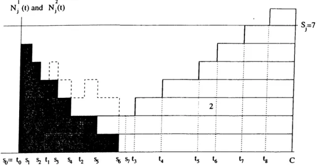
•3.5 Exhaustive CaseiTotal Inventory Process During the Cvcle Time 40 3.6 Phase-type Representation of rjiJ ^ i ... 45

3.7 Phase-type Representation of Cycle Time C ... 48

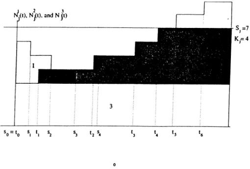
3.8 Gated Case: A Particular Realization of N j, j ^ к... 51

3.9 Gated Case:Total Inventory Process During the Cycle Time . . 52

3.10 Phase-type Representation of 7^, = Em=K, 4 j m ... 57

3.11 Phase-type Representation of 7,·, qjK, = Qjm,i ^ j . . . 57

3.12 Phase-type Representation of C, q^x, = = 1, 2. 58 3.13 G-Limited Case:A Particular Realization of jVj, j ф к... 62 3.14 G-Limited Case:Total Inventory Process During the Cycle Time 63

List o f Tables

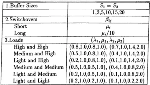
4.1 Problem generation parameters for the exhaustive c a s e ... 68 4.2 Decomposition accuracy of the exhaustive case: A summar}’. . . 70 4.3 Computation time requirements of the exhaustive case in cpu.

seconds... 71 4.4 Problem dimensions of the exact and decomposed models in the

exhaustive case... 72 4.5 Approximation accuracy of the exhaustive case: A summary. . . 74 4.6 Decomposition accuracy of the gated case: A summary... 75

4.7 Computation time requirements of the gated Ccise in cpu. seconds.. 77

4.8 Problem dimensions of the exact and decomposed models in the gated case... 77 4.9 Approximation accuracy of the gated case: A summary... 79 4.10 Problem generation parameters for the G-limited case (^i =

52 = 5, A', = A^2 = A ' ) ... 80 4.11 Decomposition accuracy of the G-limited case: A summary.. . . 82 4.12 Computational results of the G-limited case... 83

4.13 Problem dimensions of the exact and decomposed models in the

G-limited case. 84

4.14 Approximation accuracy of the G-limited case: A summary. 86

B.l Exhaustive case: Problem D a t a ... 98

B.2 Exhaustive case: Problem Data (continued) 99 B.3 Exhaustive case: Exact and decom posed ... 100

B.4 Exhaustive case: Exact and decomposed (continued) ...101

B.5 Exhaustive case: Exact and decomposed (continued) ...102

B.6 Exhaustive case: Exact and approxim ation... 103

B.7 Exhaustive case: Exact and approximation (continued)...104

B. 8 Exhaustive case: Exact and approximation 105 C. l Gated Case: Problem d a t a ... 107

C.2 Gated Case: Exact and decomposed...108

C.3 Gated Case: Exact and decomposed (continued)... 109

C.4 Gated Case: Exact and ap p ro x im atio n ...110

C. 5 Gated Case: Exact and approximation (continued) ... I l l D. l G-limited Case: Problem d a t a ...113

D.2 G-limited Ccise: Problem data/"co n /m u ed j...114

D.3 G-limited Case: Exact and decomposed...115

D.4 G-limited Case: Exact and decomposed (continued)... 116

D.5 G-limited Case: Exact and decomposed (continued)... 117

D.6 G-Iimited Case: Exact and decomposed (continued)...118

D.7 G-limited Case: Exact and approximation ... 119

D.8 G-limited Case: Exact and approximation (continued)... 120

D.9 G-limited Case: Exact and approximation (continued)... 121

D.IO G-limited Case: Exact and approximation (continued)... 122

C hapter 1

Introduction

Queuing networks have been widely used to estimate the various performance measures of production systems after 1950s. As Leung and Suri [21] points, they are most appropriate for aggregate analysis in the design phase to explore a large number of alternative system designs, and for production and capa­ city planning in the operational stage. Most of the systems can be modeled in a form of queuing network. But huge computational and memory require­ ments prevent researchers to analyze the real systems accurately. Most real life systems have various control policies, large number of machines, multiple type products, general processing, failure and repair time distributions, hence they are very difficult to model and solve as a queuing system. Thus, most researchers deals with single-item multiple-stage, or multiple-item single-stage models, in which some of the distributions are Markovian.

In this thesis, a two customer, single server polling system is considered that hcis been studied extensively to model both production systems, computer networks, and satellite communication systems. For example, in computer local area networks (LANs), the nodes represent terminals or workstations. The customers are the messages that arrive at a terminal for processing. The server is an imaginary "token” or signal that activates a terminal whose messages are then transmitted or processed. After a delay for switching, the token then goes to the next node and activates it. This represents the “token ring” type

CHAPTER 1. INTRODUCTION

of LAN protocol [28]. Another application is the stochastic multi-product production systems where the server is a machine or cell of machines and the nodes correspond to different product types by considering customers as the orders. Using polling models some performance measures can be calculated such as, thruput rate, average queue length, mean waiting time and so forth.

In polling models there are different customers which have individual arrival processes and service times. Arrivals join their dedicated queues. A server visits these queues in an order, which may be predetermined as well as random. At each visit server gives service according to a given policy. Customers for which the service is completed departs from the system. A switchover time elapses as the server moves from one queue to another.

In this thesis queuing theory terminology will be used. Products are re­ ferred cis customers, as well as machine or processor as server, and setups as switchovers.

Organization of the thesis is as follows: In the next chapter a classification of one server models and a literature review will be given. The third chapter is devoted to analyze of M/M/1 polling models under three service policies. Numerical results of the different service policies including the algorithms are provided in Chapter 4. The thesis ends with the conclusion and suggested avenues for future research.

Chapter 2

Polling M odels: A

Classification

There have been many alternative forms of polling models as seen in the lit­ erature. The common characteristics among all models are the existence of randomness. Also all works deal with stationary distributions. Most of them assume that there is only one server, although polling models find applications with multiple servers. This classification based on the articles that have been published since 1966. Although it is not claimed to be an exhaustive survey it will be very helpful in analyzing the previous works, assessing their contribution in the literature. First of all, the differentiating attributes of polling models will be analyzed. These are arrival process, service time, switchover time, polling policy, service policy, service discipline, buffer size, customer types, preemption, symmetricity, vacation and unreliability.

1. A rrival P ro c e ss is the first distinguishing element of polling models. Most of the literature deals with Poisson arrivals, but there is a work ([38]) that consider renewal processes. So interarrival times could be :

i. Deterministic, or ii. Stochastic

. Exponential,

. Phase type,

. General-continuous, . General-discrete.

Nevertheless there is no model that has deterministic, or continuous and generally distributed interarrival time in any work.

2. Service tim e has almost similar characteristics with the arrival process. Although most of the literature deals with general distributions, there are some w’ork that consider Markovian distributions. So service times could be:

i. Deterministic, or ii. Stochastic . Exponential, . Phase type, . General-continuous, . General-discrete.

3. Sw itchover T im e or setup time is a complicating element in the polling models. When server moves from one queue to another it is idle for a period of time. This period includes all the elements of preparing for another queue. Switchover times could be :

CHAPTER 2. POLLING MODELS: A CLASSIFICATION 4

i. Deterministic . Zero, . Non-zero. ii. Stochastic

. Exponential, . Phase type,

. General-continuous, . General-discrete.

There is a considerable amount of studies ([27],[14],[8]) that consider zero switchover time. Solution techniques may be different whether swithcover times are

. Queue dependent, or . Sequence dependent.

CHAPTER 2. POLLISG MODELS: A CLASSIFICATION o

4. Service policy may be the most differentiating feature of polling mod­ els. It defines either probabilistically or deterministically the number of cus­ tomers to be served by the server in a visit.

These policies can mainly be divided into two parts: dynamic policies and static policies. Dynamic policies are mostly encountered in the optimization models, where service policy is determined by the system state. But service policies are static in most performance evaluation models. In the static case the policy does not change in time, whatever the system state is. These static models are explained in detail.

There are mainly three static service disciplines that have been studied extensively in the literature: exhaustive, gated and limited. Once server begins to serve a queue, it continues until queue becomes empty, this is known as exhaustive service policy. Gated service policy is the same as exhaustive, but arrived jobs after server’s visit time are left to the next visit. Limited case refers to a fixed batch. Server always processes up to a fixed amount from a particular queue, then switches to the next queue. But there appears different policies in case of server faces with less than batch size of customers. They are explained later in this section. When the batch size is one that policy is called

as 1-Iimited or non-exhaustive. Besides, there are less popular policies which are the generalizations of the first three. Binomial-gated policy is an extension to gated one. In this policy, the number of customers served by the server is binomially distributed with parameters of n, number of customers present in the visit instant, and p, a fixed queue dependent probability. When p = 1 this policy reduces to gated one.

E-limited is a hybrid of limited and exhaustive, server decides to serve queue exhaustively or a randomly chosen number of customers are served. An example of E-limited policy is Bernoulli. After a customer is served, server decides to give service to another customer with a queue dependent probability, p, otherwise visit finishes. When p = 1 and p = 0 this policy reduces to exhaustive and to 1-limited respectively. G-limited is also a special case of limited service policy. Server serves a fixed number of customers when it finds more customers than this limit at the polling instant, otherwise he serves all the customer present at that instant and leaves the new arrivals to the next visit.

There also exist some other service policies reported in the literature. In semi-exhaustive policy server continues serving until the number of customers drops to one less of the number at the polling instant. For instance server leaves the queue if there is no new arrival until the service completion of the first cus­ tomer, otherwise he continues with the second one, and so forth. Time limited policy refers to give service in time units rather than number of customers. The distributional assumptions about the time limits adds more classes to polling models.

As a result, service policies could be summarized as follows:

CHAPTER 2. POLLING MODELS: A CLASSIFICATION 6

a. Dynamic policies, or b. Static policies

i. Bernoulli

. 0 < p < 1,

. p = 0 (1-limited or non-exhaustive). ii. Binomial gated

. p = 1 (Gated), . 0 < p < 1. iii. Limited . K = l (1-limited or non-exhaustive), . 1 < A' < 00 (A'-limited), . G-limited, . A-limited. iv. Semi-exhaustive V. Time limited . Constant, . Exponential, . General.

5. Polling Policy determines the next queue to be visited. First of all we can clcissify polling policy as dynamic and static. Dynamic policies are mostly used in optimization models. Here next queue to be visited is de­ termined by the system state. In static policies polling may be determined either probabilistically or deterministically. In the latter case server strictly follows the polling table, in the former case the next queue is selected prob­ abilistically. There are famous deterministic polling policies that extensively studied in the literature. They are cyclical ( 1 ,2 ,..., A^, 1 ,2 ,...), scan type ( l , . . . , yV- l , A^, T V a n d star type (1,2,1,3, . . . , 1, A^, 1,2,1, . . . ). There can be other policies that are predetermined, fixed, and need not be in a special form. So with respect to polling policies considered, polling models can be classified as:

CHAPTER 2. POLLING MODELS: A CLASSIFICATION

b. Static.

i. Nondeterministic, or ii. Deterministic

. Cyclical, . Scan type,

. Star type (or priority), . General.

6. Service discipline within queues adds one more attribute as in cla.ssical queuing models. It simply determines the order of customers that will be served. Service discipline in a polling model could be:

. FIFO, . LIFO,

. RO (random order),

. processing time dependent (SPT, LPT, etc.).

7. B uffer sizes are another characteristic of polling models. Solution techniques largely differ when queues have infinite, finite or single capacities. Takagi [35] points out the importance of queue capacities, therefore, queue capacities could be:

. single, . finite, . infinite.

CHAPTER 2. POLLING MODELS: A CL ASSIFICATION i

8. N u m b e r of cu sto m e r ty p es is also considered as another classification item. Earlier works mostly deal with two customer types. But applications of

polling models have been extended to multiple customer types. But a clcissifi- cation due to the number of customers is inevitable because it is not possible to adopt every solution technique for two customers to arbitrary number of customers. Hence, the number of customer types could be:

. two, or . multiple.

9. P re e m p tio n is also an important modeling feature in polling models as it hcis been in scheduling theory. Preemption is closely related with the service policy. For static service policy models talking about preemption is meaningless except for time limited ceise. In a time limited model the question of “what will be done” arises if the time expires in the middle of processing. Also in dynamic service policies the analyst faces with a similar question. Therefore, in a polling model preemption could be:

i. Not allowed, or ii. Allowed

. preempt-resume, . preempt-repeat.

CHAPTER 2. POLLING MODELS: A CLASSIFICATION 9

If preemption is not allowed, server completes his current work and then he proceeds regularly. If the preemption is allowed, there are tw'o cases: If system is preempt-resume, server leaves his work and when returned to the same cus­ tomer he continues his service for the remaining work. In preempt-repeat case server begins service from the beginning. If the service time has a stationary memoryless distribution these two Ccises are probabilistically equivalent.

10. S y m m e tric vs. n o n sy m m etric distinction is very important in a- nalyzing polling models. When the customers have the same characteristics the system is called symmetric. Symmetric systems are obviously easy to

CHAPTER 2. POLLING MODELS: A CLASSIFICATION 10

analyze. There are some works that express the weighted average of waiting times of customers as system parameters. Such representatipns is called pseudo­

conservation laws. When the system is symmetric one can easily calculate the

various performance measures of the system in closed forms. Hence, the system could be:

. symmetric, or . nonsymmetric.

11. V acation is another complication that is added to the polling models. When the system is empty, there are no customers waiting or being served in any queue, a random vacation is scheduled for the server. The distributional assumptions on vacation periods add more classes to the polling models. But there is little work that assume vacation in the model. So, the system could be: i. Without vacation, or 11. With vacation . exponential, . phase-type, . general-continuous, . general-discrete.

12. U n reliab ility of the server adds another complication to the polling models. Although most of the literature assumes no failure of the server, unreliable servers may be suitable to model production systems where some machines are failure prone. Also, the assumptions about failure and repair time distributions can add more classes. In a polling model, server could be:

CHAPTER 2. POLLING MODELS: A CLASSIFICATION 11

ii. Unreliable, and associated distributions could be . exponential,

. phase-type,

. general-continuous, . general-discrete.

After this classification it will be eaisier to understand the real assessment of earlier works and our models.

2.1

L iteratu re R ev iew

Although there are several classes of polling models, studies in the literature are not so evenly distributed among various classes. Instead, the most of the polling models assume that arrivals are Poisson, service and switchover times are generally distributed. Furthermore queues have no limit, they have infinite capacity, number of the queues are more than two. Also service discipline is FIFO. Usually all models fulfills these assumptins. It will be pointed if there is a deviation from these assumptions. While reviewing the literature it is beneficial to divide them into two categories. Infinite queue polling models are reviewed first.

2.1.1 In fin ite Q u eu e P o llin g M od els

The earliest work, we are aware of, is due to Skinner [30]. He worked on a two queue system where switchover times consist of a variable and a constant por­ tion. He classifies queues as low priority and high priority. His policy is simply serving high priority queue exhaustively, and low priority queue as 1-limited. He first analyzes an M / G / l queue with vacations and adopts his results to the two queues system. He found the exact Laplace-Stieltjes transform of the wait­ ing time distribution and probability generating function of the queue length

CHAPTER 2. POLLING MODELS: A CLASSIFICATION 12

distribution. He also states the stability conditions. Durr [10] analyzes a two- queue system, where one queue heis priority over the other. That is whenever high priority customer exists in the system it is served immediately. He con­ siders exponential service and negligible switchover times. He worked on both preemptive and nonpreemptive case and found that:

Var{\\'i : F I F O ) < Var(Wi : RO) < V ar{W i: LIFO)

where Wi is waiting time of the ¿th customer type. Sykes [3.3] is among the first that include nonzero switchover time. Mean waiting, mean queue length and average busy period are found for exhaustive service in both queues. ' Eisenberg [11] works on two queues polling system under alternating prior­

ity and strict priority. Alternating priority is simply exhaustive Ccise. In strict priority, the customer type is served immediately «is it arrives. Preemptive case is also considered. He obtains mean waiting time and mean queue length. In a later work [12] he finds Laplace-Stieltjes transform of the waiting time dis­ tribution, with more than two queues under exhaustive service discipline. He also provides a method to calculate the means of the performance measures. It is the first study analyzing more than two queues

More recent works usually consider arbitrary number of queues and more general polling and service policies. Manfield [23] uses a polling model to find the mean w'aiting time of messages that arrives to and departs from a cen­ tral device. Departing messages are generated by the processing of incoming messages, and he argues that outgoing messages are also Poisson and con­ jectures that outgoing messages should have high priority over the incoming ones in order to refrain from deadlocks. A star type service discipline is as­ sumed. He polls incoming messages non-exhaustively, and outgoing messages non-exhaustively or exhaustively. He finds the Laplace-Stieltjes transform of the waiting time distribution and argues that analysis of outgoing messages is exact, but others are approximate. Boxma et al. [5] provide a pseudoconser­ vation law for cyclical polling models where different service policies applied for queues. In the literature pseudoconservation law is defined as an expres­ sion for the weighted average of mean waiting times. They are particularly

CHAPTER 2. POLLING MODELS: A CLASSIFICATION ₁₃

important to find performance measures of symmetric systems and checking the correctness of the analytical solutions. Boxma et al. [5] assume discrete time queues where interarrival times, service times and switchover times are generally distributed. They also convert their law to continuous case by apply­ ing a limiting procedure. They applied their law to the star polling policy and agree with Manfield [23]. Giannakouros and Laloux [15] generalizes the work of Manfield [23] using the results of Boxma et al. [.5]. Constant switchover time is assumed. They model the system when low priority queues are polled not only non-exhaustively but also exhaustively and gated. They showed that non- exhaustive case is very accurate when the traffic intensities are low or medium, and exhaustive and gated cases are very accurate for the whole class of traffic intensities. They also report some numerical results. Takagi and Murata [36] give an exact analysis of waiting time in scan type policy. In their models, service times are constant and interarrival and switchover times have general discrete distributions. They considered three service disciplines, time limited, in which switchover times are assumed to be zero, gated and exhaustive. They also compared these policies with respect to their mean waiting times. Levy [22] finds a pseudoconservation law for cyclical polling system where service policy is binomial-gated. He also finds the control variables, p,’s so as to min­ imize the sum of weighted waiting times. Watson [40] gives conservation laws for exhaustive, gated, and and non-exhaustive service disciplines. He also gives a brief survey of the work on polling models.

Sarkar and Zangwill [^8] calculate mean and variance of cycle time more effectively than previous works. They also note some applications of polling models. In further work [29] they study the effects of processing time and switchover time variation on the system performance. They conjecture that variability play a central role in effective capacity through some paradoxical examples.

Takagi [34] gives a unifying work that considers general priorities within queues in a cyclic polling system. These priorities are FCFS, RO, LCFS, shortest processing time (SPT). That work also studies preempt-resume and nonpreemptive systems.

CHAPTER 1 POLLING MODELS: A CLASSIFICATION 14

Ibe and Trivedi [17] study a two-queue case where the server is subject to breakdowns. Failure times are exponential and repair times are generally distributed. They obtain approximations for mean waiting times for 1-Iimited service policy.

Leung [20] studies on an exponential time limited polling model. He con­ struct an embedded Markov Chain at the visit beginning, visit completion, service beginning and service completions epochs. Waiting time and queue length distributions are found using discrete Fourier Transform. Exponential time limited policy is compared with constant time limited and k-limited poli­ cies.

Aforementioned works consider static service policies. But considerable works are studied for optimization models through dynamic service policies. Blondia [4] studies a polling system where polling is made dynamically. Queues are assigned some priority, and after each service completion next queue se­ lected according to this priority. System is nonpreemptive. When the system becomes empty server takes a vacation that is generally distributed. Steady state queue length distribution and Laplace transform of the waiting times are obtained.

Cohen [8] studies a two queues system, where switchover times are assumed to be zero. Service policy is a dynamic one, after each service completion, server visits the queue that has the largest number of customers waiting for service. Tie5 are broken randomly with predetermined probabilities.

Boxma et al. [6] construct a model to find the optimal visit frequencies of queues in cycle, so as to minimize the sum of weighted waiting times. Since the optimization problem is very hard to solve they propose an approximate method. Also they propose a way to distribute these frequencies evenly in a cycle. They give extensive numerical results to investigate how far away their method from the optimal solution for service policies exhaustive, gated and 1-limited.

CHAPTER 2. POLLING MODELS: A CLASSIFICATION ₁₅

Srinivasan [31] works on a nondeterministic polling system. Server, follow­ ing service at station i, either polls station j with probability pij if there is a service at station i, or polls station j with probability e,j if there is no service at station i. Obviously pij = 1 for all i and JZj = 1 for all i. He works on exhaustive, non-exhaustive, gated and semi-exhaustive service policies. He obtains expected cycle time and stability conditions. He also provides pseu­ doconservation laws for two special cases: = e,j with arbitrary number of queues and, two stations with arbitrary p.j’s and e,j’s. Mean waiting times are found for exhaustive and gated service disciplines. System performance can be optimized through playing with these probabilities.

Altiok and Shiue [2] analyze a multi-item (R,r) inventory policy under the assumption of backorders. Production is requested when the inventory in front of the machine drops to r. When there are two such products higher priority products produced first. They approximate the average queue level and backorder level. Their model is simply a polling models with a dynamic polling policy and exhaustive service policy.

Blanc [3] considers a cyclic polling system with Bernoulli service policy. Ex­ ponential service times and negligible switchover times are assumed. A method is proposed to find queue length distributions and waiting time distribution without explicitly solving the underlying Markov Chain.

Hofri and Ross [16] investigate the optimal control of two queues where idleness is allowed. Processing times are generally distributed but identical for all queues. They considered two objectives: minimizing the sum of discounted holding cost and switching cost, and long-run average of the sum of holding and switching costs. They construct a Markov decision process where decision epochs are made in service completion, switch completions and arrival points when the server is idle. They show that optimal policy is exhaustive for dis­ counted cost criterion. They further conjectured that this result is natural because service times are identical for all customers. They also showed that server should not switch unless one of the queue length reaches a threshold

CHAPTER 2. POLLING MODELS: A CLASSIFICATION 16

value. They also show that such a double threshold policy is optimal for aver­ age long run cost criterion. And finally an algorithm is proposed to find these threshold values.

Campbell [7] reviews some of the important works and summarizes some of the important results reported in the literature. He also clarifies the distinc­ tion between cyclic server models (polling models) and cyclic customer models (closed queuing networks).

2.1.2

F in ite Q ueue P ollin g M od els

Finite queue polling models have attracted considerably less researchers. It may be due to two reasons: They are very difficult to analyze exactly, so they require more assumptions and they may have less application area. Neverthe­ less, a number of finite queue models exists in the literature. In all finite queue models, it is assumed that customers who find the queues full are lost.

Takine et al. [37] give a unified approach to polling models with single ca­ pacity buffers. They study both exhaustive and gated service policies. Mukher- jee et al. [24] improve the work of Takine et al. [37]. They construct a Markov chain embedded at the time instants when stations are polled. Instead of solving all equations, they propose an iterative algorithm.

Tran-Gia and Raith [39] analyze a multi-queue system where arrivals are Poisson, service times and switchover times are generally distributed. But switchover times are queue dependent. Furthermore polling policy is cyclic and service policy is non-exhaustive. They construct an embedded Markov chain. While doing so they find the mean and variance of the cycle time of each queue, and approximate it with a two stage phase type distribution. They also test their algorithm via the computer simulations.

Takagi [35] gives an exact analysis of polling models where arrivals are Poisson and service and switchover times are generally distributed. It is the first work that gives a unifying approach to finite queue polling models. He

CHAPTER 2. POLLING MODELS: A CLASSIFICATION ₁₇

considers three service policies: Exhaustive, gated and G-limited. He uses the results of earlier works on single server, finite capacity vacation systems. These works begin with constructing a Markov Chain embedded at service completions and visit beginnings. So, he decomposes the system by assigning vacations when the server is processing the other queues. His approach requires a considerable amount of numerical integrations and inverse Laplace-Stieltjes transforms. The computational tractability of that approach is very low, and hence numerical results are not reported.

Tran-Gia [38] presents an approximate algorithm for polling systems with finite queues, cyclic polling and 1-limited service. All distributions are general but discrete. Therefore, convolutions are made using the fast Fourier transform. Although his model is applicable for nonsymmetric models, the analysis is made for symmetric load conditions. The approximation accuracy is tested with computer simulations.

Albores and Bocharov [1] consider two finite queue with relative priorities, where interarrival and service time distributions have general phase type rep­ resentations. Switchover times are assumed to be zero. They consider three service disciplines: FIFO, LIFO and RO. Their result is a matrix-algorithmic approach to solve the steady state probabilities.

There are also finite queue optimization models. For example Suk and Cassandras [32] consider the optimal scheduling of two queues competing for one server. There is no switchover time and interarrival and service times are exponentially distributed, furthermore idleness is not allowed. They find that the policy minimizing the total discounted blocking cost and inventory holding cost is of a switching type when the blocking cost is greater than the unit inventory holding cost. Switching type means customer type is served depends on the number of customers waiting for the service.

Rosberg and Kermani [27] deal with scheduling N queues on a single server that maximizes the sum of weighted thruputs of the customers. Arrival pro­ cess is assumed to be Poisson and service times are exponential. Furthermore switchover times are assumed to be zero. They first find an upper bound to

CHAPTER 2. POLLING MODELS: A CLASSIFICATION 18

the value function by decomposing the system and propose two approximate schedules. They also test the performance of their approximate schedules.

Works on finite queues polling models are scarce in the literature. Also there is little implications about the solution techniques. But there is no work that exactly matches with our models which will be described and solved in the next chapter.

C hapter 3

Two Q ueues M /M /1 Polling

M odels

3.1

In tro d u ctio n

As we see from the previous chapter, most of the works in the literature deals with polling systems, with infinite queue capacities. But it is easily seen that there is a lack in finite queues even in Markovian systems, where all the dis­ tributions are exponential or of phase type. In this chapter various polling policies are studied under Markovian distributions. Before going into details, it will be beneficial to state the major assumptions:

All the random variables are assumed to be exponential.

Switchover times are sequence dependent rather than queue dependent, . Idleness is not allowed,

. Polling policies are deterministic and cyclical. . Service disciplines in queues are FIFO.

. Buffer sizes are finite.

CHAPTER 3. TWO QUEUES M/M/1 POLLING MODELS 20

. Customers finding full buffer are lost, . There are two types of customers, . Preemption is not allowed,

. Server is assumed to be reliable and always ready to operate.

In this study three service policies are considered, namely exhaustive, gated and G-limited.

3.1.1

N o ta tio n

Since the same notation is used throughout the thesis, it would be beneficial to give the common notation at the very beginning.

Xj is the rate of the arrival process of customer j , j E J = {1,2},

Yj is a random variable (r.v.) representing the processing time of customer j G 7, exponential with rate pj,

Xij is a r.v. representing switchover time that customer exercises going

from customer i to customer j , exponential with rate i , j 6 J and i ^ j ,

S j is the capacity of the queue that customer type j joins (excluding

the one in the service, if this queue is being served).

> 0} is a stochastic process that represents the number of cus­ tomers type j , in its queue at time t, where Nj{t) G Ej = {0,1, . . . , Sj}.

{Z{t), t > 0} is a stochastic process representing the state of server at time t, where Z{t) G E z = {1.2,3,4), and

Z{t) =

1 server processing customer 1 2 server processing customer 2

3 server switching from customer 1 to customer 2 4 server switching from customer 2 to customer 1

CHAPTER 3. TWO QUEUES M/M/l POLLING MODELS 21

Furthermore,

Pjm represents the steady state probability of m customers being in queue j , THj is the steady state throughput rate of customer j,

3.1.2 Organization

In this chapter the steady state performance measures of polling systems is found under mainly three service policies. First section is devoted to exhaus­ tive service policy. In this section a Markov Process is defined and its embedded Markov Chain is constructed to calculate the steady state probabilities. Also system is decomposed into two sub-systems that have single server and single customer type, defining imaginary vacations on servers. Furthermore the sec­ ond approach is simplified in order to get an approximation. Numerical results concerning the approximation accuracy and computational savings gained from decomposition will be presented. The succeeding chapters are devoted to gated and G-limited service policies with the same steps.

3.2

E xhaustive Service Policy

3.2.1

Exact M odel

As explained previously, in exhaustive service policy, server alternates between queues whenever the server finds no part in the queue that is currently being served. So the stochastic process {Nj{t), Z{t)^t > 0, j € J } is a Markov process with the state space E = E1X E2X E z , where \E\ = 4(5i -f 1)(5'2 1).

A particular instance {ii,t2,k) means that there is ii number of customers in

queue 1, ¡2 number of customers in queue 2, and server isjn state 1* € {1, 2,3,4}.

CHAPTER 3. TWO QUEUES M/M/1 POL '.ING MODELS 2 2 transition rates: P { i i , Í 2 , k ) { i i + l , Í 2 , k ) _{= A,} for *1 ^ S \ , t 2 € E 2 , k € E z , P { i i J 2 , k ) ( i u Í 2 + l , k ) = A2 for *2 ^ ‘^2,^1 € E \ , k G E z i 1)^2) 1) = f^l fo r *1 7^ 0, ¿2 G £'2, P ( 0 , 2 2 , 1 ) ( 0 , ¿ 2 , 3 ) ₌ for _{* 2 € £ 2,} P i i u Í 2 , 2 ) { i i , Í 2 - 1 ,2 ) = for h 7^ 0 ,¿ i G £ 1, P ( z „ 0 , 2 ) ( ¿ , , 0 , 4 ) = t^2 for *1 € £ 1, P i i i , Í 2 , 3 ) ( i u Í 2 - 1 ,2 ) ₌ ^ \ 2 for *1 Ç £1, *2 ^ 1, P ( ¿ „ 0 , 3 ) ( f , , 0 , 4 ) _{= A 2} for _{*1 £ £ 1,} P ( 2 , , ¿ 2 , 4 ) ( ¿i - 1 ,¿ 2 ,1 ) ₌ h \ fo r ¿2 G £2, i \ > 1, P ( 0 , ¿ 2 , 4 ) ( 0 , ¿ 2 , 3 ) = ^21 for ¿2 € £ 2.

where P{ii,Í2^k)(i[,Í2ik') represents the entry of the infinitesimal generator

for which the process goes from state (¿1, ¿2, k) to state (z'l, ¿2, k').

The construction of the infinitesimal generator will be explained in more detail. The first two equations state that new arrivals join their queues if they are not full with their arrival rates. The next two state that there are departures from the queue 1 with the completion of a service. In the first one server continues processing if there is at least one customer in queue 1, in the second one the server goes to switchover if there is no customer left in the queue 1. The next two simply same for queue 2. The last four equations are about the switchovers. In the first one server begins processing queue 2 after he exercises a switchover with the rate of I3\2· But if there is no customer in queue 2 it exercises a second switchover to return to queue 1. Last two are also similar.

After constructing the infinitesimal generator, P, it is trivial to find the steady state distribution of queue length and average throughput rates. Since all the states communicate, chain is irreducible and positive recurrent, the steady state distribution of states exists.

Let, r(¿i,í2,^) be the steady state probability of state (fi,¿2,A'), and r be the corresponding vector. So, the solution to the following system of equations,

CHAi’ TER 3. TWO QUEUES M/M/l POLLING MODELS ₂₃

r/> = 0 _(3.1)

(3.2) E r = l

t€E

provides the required probabilities. Average throughput rates and queue length distributions can also be obtained eiisily, as follows:

THj = Hj r(n i,n 2,;) ni ,U2 P \ m = Y r { m , n2, k ) ri2,k P2m = Y r { n i ; m , k ) ni,k (3.3) (3.4) (3.5)

If one stores all the elements of the rate matrix P, memory requirements will be O(jjE'p), and computation time will be about 0{\E\^), to solve steady state probabilities by Gaussian Elimination. But rate matrix is quite sparse, approximately three nonzeros per row. Therefore the sparsity is exploited using a sparse solver with enormous savings in both computation and memory requirements. The use of sparse solver will be explained in detail in numerical computation section.

3.2.2

D eco m p o sitio n

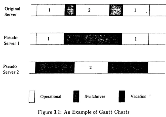
The aim of the decomposition is to reduce the problem into a manageable size. The approach is a very simple and widely used. The system is approximated with two one-server queues, defining new pseudo-servers to represent the be­ havior of the original server. To accomplish this task, vacations are scheduled for the pseudo-servers in order to model the switching of the original server. When a buffer becomes empty, a vacation is scheduled for its pseudo-server. The primary task is to determine the distributions of these vacations, which will be explained in the following subsection. Figure 3.1 can help to better understand the decomposition methodology.

CHAPTER 3. TWO QUEUES M/M/1 POLLING MODELS ₂₄ Original Server Pseudo Server 1 Pseudo Server 2

I I Operational | | | | Switchover H Vacation

Figure 3.1: An Example of Gantt Charts V acation P erio d s

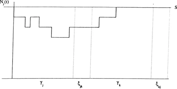
When server finishes serving a queue in a cycle, it switches to the other one. Now, vacation for the pseudo-server begins. A switchover time elapses, while server is set up for the other type of customer. Server turns back after it finishes all the jobs in the second queue. Server begins to serve the first queue after a second switchover time is also elapsed. This is end of the vacation of the pseudo-server as well as the beginning of a new cycle. Same process applies for the second queue. Let

be a r.v. denoting the vacation period of pseudo-server j, in cycle /. So, it is clear that:

= Xi2 + 72 ^ + ^21 (3-6)

T)2^ = A21 + 7 i ^ + '^12 (3 - 7 )

w’here 7]^^ is a r.v. denoting the time required to finish all customers in queue

j , in cycle /. It will be called as clearance time.

CHAPTER 3. TWO QUEUES M/M/1 POLLING MODELS ₂₅

distributions for 'fj'K If 7j ‘^ —^ ' / j a s l —^oo then it is obvious that rjj‘' —> rjj as / —> oo. The existence for the invariant distribution of clearance times will be questioned later in this section. For the time being it is assumed that the distribution exists.

Let be the clearance time when the server visits queue j and faces with

k customers in the queue, then it is obvious that:

A‘)

Ij = S

i 7 j “’ with probability qjo 7 '·’ with probability qji

('t)

7y with probability qjk

U with probability qjSj

(3.8)

where qjk is the probability of being k customers in queue j , when the server is ready for the processing customer type j, and qjs^ = YlT=Sj Notice that there cannot be more than Sj customers, independent of the number of arrivals during the vacation time.

Suppose that there are k customers at a time. If a new arrival occurs before the first service completed (with probability Aj/(^j + Ay)) then clearance time will be as if there are (k + 1) customers. This follows from the memoryless property of the exponential distribution. If the service is completed before a new arrival (with probability + Ay)) then clearance time will be sum of the service time of the customer (Vy) and clearance time as if there are (A: — 1) customers. With this idea following system of linear equalities is derived as follows:

v(0) _= 0

7 0 ) = 7 f =

CHAPTER 3. TWO QUEUES M/M/1 POLLING MODELS ₂₆

Figure 3.2: Phase-type Representation of j j j ^ k

^ = Pi!(Pj + (k-l) + >S) + ^j/(Pj + ^ j h j

7]^^^ - PjliPi + + ^j) + ^j/{pj +

If one takes the e.xpectation of both sides in above system of linear equal­ ities, a system of linear equations can be obtained, where there are { S j -b 1)

variables and { S j -t-1) equations. £'(7]^^) for k = 0, ...,5j can be obtained

eas-/ L\

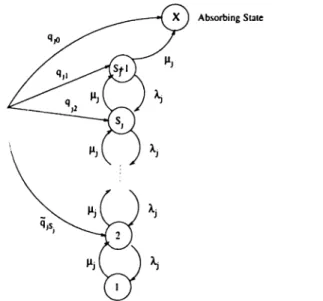
ily. In general, it is possible to get the Laplace transform of the 7] 's. In the above argument all the properties of exponential distribution are not exploited, instead there is a more rigorous method to find the distribution functions of not only clearance times but also vacation periods.

A phase-type distribution can be defined with a Markov process, in which all states are transient except the absorbing state and an initial probability vector. Figure 3.2 represents the states of the distribution of 7j. States 1 through S j -b 1 represents the number of customers in the system in reverse

order. State X is the absorbing state. Therefore clearance time of pseudo­ machine j is the time elapsed the process reaches to state X. Initial probability vector of this distribution is (0, qjs^, qjSj-i·, · · ·, 9jo)· As a result if qjUs are

CHAPTER 3. TWO QUEUES M/M/1 POLLI.\G MODELS ₂₇

estimated, complete description of can be obtained. Notice that vacation period is nothing but a convolution of two switchovers and the clearance time of the other queue. Neuts [2-5] states that convolution of phcise-type distributions are also phcise-type.

If vacation period of pseudo-server 2 is given, i.e., T, then it is obvious that

9 » = e -*>^ (A ,r)‘ / i ! . i = 0 , l , . . ¿ V j - l , h s ,

=

e-">^(A

r)V*!.

k=S2

which corresponds to Poisson distribution. But vacation period of each pseudo­ servers is a random variable that has phase-type representation. So, general­ ization easily follows.

q,k

= r (e -" '“(A,u)Vi!)/„(u)¿u,t = 0, l , . . S , - l ,

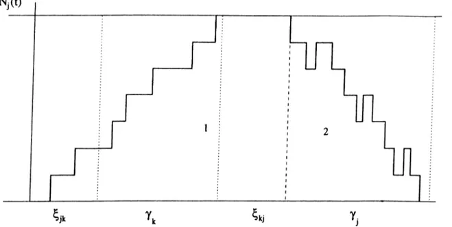
As it is noted earlier rjj has a phase-type representation as it is shown in

Figure 3.3. Let Qj be the infinitesimal generator of corresponding Markov Chain, with the state space, { 1 ,2 ,..., Sj -I- 3,X}. As Neuts [25] states Qj has the following form:

' Aj AO,

0 0

Q , = (3.10)

where the {Sj -f 3) X {Sj -|- 3) matrix Aj hcis negative diagonal and positive off-diagonal entries. Also Aje -|- = 0, and the initial probability vector of

Qj is given by (q j,9j-). with qje -f = 1. But all states except state X should

be transient, that is absorption into the state X should be certain. Sufficient condition is simple : \ j < Hj. Now it is time to determine Aj and the initial probability vector

CHAPTUR 3. TWO QUEUES M/M/l POLLING MODELS 28

Figure 3.3: Phase-type Representation of Tjj j ^ k

The matrix Aj, that is nothing but the infinitesimal generator of the Markov Process, is: -Pi Pi 0 0 0 0 0 A. —(A, + Pi) Pi 0 0 0 0 0 A.· ~ (A , + /i,) . . 0 0 0 0 0 0 0 • ~ ( A , + Pi) Pi 0 0 0 0 0 A. - { p i + A,) Pi 0 0 0 0 0 0 0 0 0 0 0 0 _{- A i}

where i / j. Notice that the switchovers are added as + 2)nd and (5^ +3)rd states. The initial probability vector is:

Hi = (O' , <7jS, -1, · · · · 9ji, 9jo, 0)

As Neuts [25] states. /,,(« ) = exp(.4,u)A°. This is the crucial point to find qjS, because system of equations (3.9) reduce to a system of linear equations with S1+ S2 + 2 equations and 5i + 52 + 2 unknowns. From the above

CHAPTER 3. TWO QUEUES M/M/l POLLING MODELS 29

arguments it is clear that there exists stationary distribution for clearance times if qfk as / —+ oo. Let us rewrite equations 3.9 by incorporating the cycle index, = f

^^“(Aju)^/^!)qf^exp(Aju)Aj*<fu,

+QiS. f (e"^^“(A _ ,u )V ^ !)eiS jex p (A ju )A ? d u ,

for i j e J , i ^ j , k = 0,1, . . S j - 1, oo 5, aoo = E (e-^^“(A,u)V^!)eimexp(Aju)A?du, OO .QO + E i i S / (e"^J“(A _ ,u )V ^ !)eiS je x p (A ju )A ? d u , k = S j for i j e J , i ^ j , (3.11)

where ejni is a row vector of appropriate size that hcis all zeros except the entry corresponding to q·^, which is one. Let,

ajmi = f (e” ^^'‘(Aju)V^!)eimexp(Aju)A?du,

for ^ J ·) ^ ^ ^ snd

^jmS-■j = E <*J”**’ i ^ and m = 0, 1, ...Si. A*=5,

Then Equations 3.11 become :

5 .-1

¡1^" = E f . ' l V » + fof ■·> e ^ i = and. 1,k

CHAPTER 3. TWO QUEUES M/M/l POLLING MODELS ₃₀

5 ,-1

= Y i <7.2¿jm5, +qis,ajs,s,, for i j € J, i / and, (3.12) m=0

Therefore aferomentioned linear system is obtained. Following theorem states the existence of limiting qjkS.

Theorem 3.1 ^ 9j as I oo for j 6 J

Proof: Let,

Ti =

ajoo Ojio .. • ^jmO ÛJ5.0

Ojoi Oju : . • ^jml Ûİ5.1

ajok ajik djmk · • · ajs.k

âjos, âjiSj . ·. ^jmSj · ■■ · ^jS.Sj

Above system of equations 3.12 can be rewritten in matrix form as:

1

J

q ? J

(3.13)

Notice that.

5 , - 1

^ ^ ajmk T âjmSj — 1) for i , j € «/, i Ji and m 0, 1, . . . , Si-

k=0

That is the sum of the columns are one. Hence, the matrix in Equation 3.13 is a Markov matrix. Since aj^k > 0 for all j € J·, and m = 0, 1, . . . ,5", all states are communicating and chain is positive recurrent and all states has period two. Due to Çınlar [9] there exist stationary probabilities satisfying

CHAPTER 3. TWO QUEUES M/M/'· POLLING MODELS 31

As a result, the existence of stationary vacation period distributions is proved the complete description of the system is obtained. But, finding the ex­ act parameters of the Equations 3.12 requires excessive amount of calculations. It is also possible to have an ill-conditioned system, because the magnitudes of the entries can be in very different scales. Instead, an iterative algorithm is proposed to find qjk's. Before going into details of the algorithm, a theorem will be presented. This theorem gives a simple way of calculating the qjCs. The proof can be found in Neuts [25].

T h eo re m 3.2 Let at = /k\dF{u) for k > 0, and F{u) is a phase type distribution with representation ( o r , T), where a is the initial probability vector and T is the rate matrix, then {a;t) is a discrete phase type density with representation given by

ß = X a i X l - T ) - \ S = A (A I-T )- 1 (3.14)

Neuts also provides an efficient way of computing the density {ajt} by eval­ uating vectors

and

also.

i/(0) = or/A, i/(^-f-1) = i/(Ä:)S, for k > 0,

Ö0 = and Ok = ¡^{k + 1)T^, for k > 0 ,

(3.15)

a, =1 Xi/{k -b l)e, for ^ > 0. i=k+l

where e is a column vector of ones.

An iterative algorithm is given below to find the qjk's using the above results. The algorithm is a fixed point algorithm, which stops after differences between two successive iterations are less than a fixed and predetermined c value. If this criteria is not satisfied it it terminated after a fixed number of

CHAPTER 3. TWO QUEUES M/M/1 POLLING MODELS ₃₂

iterations are performed. These probabilities make possible to find the vacation periods of pseudo-servers as well <is help to model the decomposed systems as Markov processes.

A lg o rith m 3.1

Step:=0;

approximate: =false;

q % : = l / { S i + } ) : f o r j = 0 , h . .

w hile n o t approximate and

for k = < S\ do V2 — ~ T2) * = t.;7? j f i r ' = Step+1 /» Vi = Qi / M for A; = 0, ^ < 5"2 do V\ = V \ \ 2{ \ 2l — T \)~ ^ = v,T^, = ^2Vie , S j , j € J (Step < MaxStep) do , Sicp+1 Stept

if ^*1 sLp^u - < c for each k th en

approximate :=true; Step:=Step+l:

if approximate=true th en

set as steady state probabilities for each k and j and re tu rn Step

else

re tu rn a message of failure end.

In computing <’2 = “ T2) ' and v\ = v \ \2{ \2l ~ T\) * explicit

inverses of the matrices are not used, rather v f s are solved by Gaussian elim­ ination. Since the matrices { \ \ I - T2) and (A2/ - Tx) are tridiagonal, the

CHAPTER 3. TWO QUEUES M/M/l POLLING MODELS ₃₃

computational complexity is 0{ S j ) operations. For one step there are 0 ( 8 1 8 2 }

operations. Furthermore, no row interchanges are required because matrices are diagonally dominant.

Algorithm 3.1 simply solves the system of equations 3.13 recursively in the following manner:

^ 0+1) _

q t " = and.

(3.16) (3.17)

Following theorem states the convergence of the Equations 3.16 and 3.17, thus convergence of the Algorithm 3.1.

T h eo re m 3.3 Equations 3.16 and 3.17 converges.

P roof: The same idea in the proof of Theorem 3.1 will be used. Let us rewrite the equations 3.16 and 3.17 as.

q(l+l) ^ TjT iqj", for i , j _(3.18)

where

T,Ti =

J ^ __I ^

X^m=0 ^jmO^iOm "f" !Cm=0 "1“ ^j»5,0^il5, JTm=0 ^jml^iOm "1“ ^j5|l^i05, JTm=0 "1“ ^j5,l^il5,

5Zm*=0 ^jmSj^iOm “f" ¿j5,5j^i05, Ylm=0 5 .-1 "f" ¿j5,5j^il5»

E 5| — 1 I m=0 ^ j m O ^ j S j T T i i ^jS|0^i5j5. E 5| — 1 I m=0 i Oj5|l^i5j5, E 5| — 1 I m=0 ^ j m S j ^ i S j T T i r 0;5,5j^i5;5,

CHAPTER 3. TWO QUEUES M/M/1 POLLING MODELS ₃₄ Notice that S j - l s.-i s.-i ^ y ^ y ^ j m k ^ i n m "t" ^ j S , k ^ i n S , } "h ^ ^ j m S j ^ ^ i n m T ûj5,5jÖınS, ^=0 m=0 m=0 5 ,-1 5;-l s.-l = ^ ( ^ 2 ^ j m k C ' i n m + O j m S j O i n m ) “1“ ^ ^ ^ j S t k ^ i n S t “f“ ^ j S i S j ^ i n S i ^ m=0 Jt=0 m=0 5.-1 S j - l 5,-1 ~ ^ 2 ^ 2 "f· Ö j m S j ) 4" Q|'nS, ( ^ 2 ^ J S , k 4" ^ j S , S j ) i m=0 Jt=0 k=0 5.-1 — ^ ] f ^i nm (1 ) 4- â ı n S , ( l ) m = 0 = 1, for n = 0,1,..., S j .

That is the sum of the columns adds up to one. So, the matrices {T1T2)

and {T2T1) are Markov matrices. Since ajmk > 0 for all j G J, and k =

0 , 1 , . . . , S j , m = 0 ,1 ,..., S',· and all states are communicating the chains are

ergodic. □

Hence, the stationary probabilities exist, resulting the algorithm finds the steady state probabilities of a Markov chain as if multiplying matrices by them­ selves until difference between probabilities at successive steps becomes in­ significant. Thus, the Algorithm 3.1 converges. The convergence rate of this algorithm can be found in Çınlar [9].

D ecom posed M odels

Let the stochastic process {Zj{t),i > 0}.j' G J representing the state of the pseudo-server j where Zj{t) e Ez, = {1 .2 ,---- 5, 4- 4}, ?' G J and i ^ j , such that

CHAPTER 3. TWO QUEUES M/M/I POLLING MODELS ₃₅

ZÁt) = {

1 pseudo-server j processing customer j at time t,

2 pseudo-server j is at vacation at time t, (original server is in switchover),

2 -f· ^ pseudo-server j is at vacation at time t , k = 1 ,2 ,..., 5, -|- 1, * 7^ (original server is clearing the other queue),

Si -f- 1 pseudo-server j is at vacation at time t (original server

is in switchover to return back),

Therefore, we can model the one server models as stocheistic processes

> 0},^ € A particular instance (i,k) means that there is i number of customers in queue y, and pseudo-server j is in state k. Since vaca­ tion periods are of phase type, these processes are Markov processes with state space Ej = E jXE zj where \E[\ = (5i -f l)(5'2-|-4) and j^'^l = (5"2 + l)(S'2 + 4).

Markov Chains of the above Markov processes can be easily constructed as follows:

P^{i,k){i + l , k ) = Ai for S \ , k £ E z i ,

P i ( i ', l ) ( * - l , l ) = /^1 for i > 1, Fi(0,l)(0,2) = //1

Pi(f,2)(i,4) = 92,5./^i2 for i e El,

Pi{i,2){i,k) = q2,(S2+A-k)^i2 for i G El, 5 ^ A: ^ S2 -|- 4,

Pi(¿,¿)(¿,A :+l) = /12 for i G El, 3 k ^ S2 -f· 3,

P i { i , k ) { i . k - \ ) = A2 for i £ Ei,4 < k < S2 + 3,

A ( i ,* ? 2 + 4 ) ( f - l ,l ) = ^21 for i > 1,

Pi(0,52-l-4)(0,2) = y32i.

where P{ii,k){i\,k') represents the entry of the infinitesimal generator for which the process goes from state {i\,k) to state (e'i,¿').

The construction of the infinitesimal generator will be explained in more detail. PI is the generator of the Markov process of the system where pseudo­ server 1 is operating. The first equation states that new arrivals join queue 1 with rate Aj. if the queue is not full.The next one states that there are departures from the queue 1 w'ith the completion of a service. Third equation