An Extremum Seeking Estimator Design and Its Application to
Monitoring Unbalanced Mass Dynamics
Melih Cakmakci1, Member, IEEE and Stefan Ristevski1
Abstract— When sensor information of a controlled-system output is not available, estimators can be used. Estimators are algorithms that take the available sensor data from the system and estimate the necessary data to be used by the feedback controller. Typically, estimation is done by running a model of the plant inside the controller and formulating an output error minimization mechanism to calculate the unknown dynamics and parameters. In this paper, a new estimation mechanism based on extremum seeking is presented. The method utilizes the idea of minimization of a non-linear error function of written in a specific structure, which may be suitable for systems with periodic dynamics such as systems with unbalanced masses. An estimation adjustment algorithm can be built based on the error between the model outputs and the actual sensor data. This adjustment algorithm drives the error between the model and the actual plant output to zero, while the feedback controller uses the information from the model. This proposed method is then applied to a mobile robotic system to improve its locomotion. Our initial results showed promising improvements up to five times more displacement with the same command on a testbed environment with challenges in eluding high-order dynamics and digital effects at high-frequency input.
I. INTRODUCTION
Sensors are devices in which the designers utilize funda-mental mechanical, electrical, or chemical results to monitor the output of a physical system. Sensors are the primary components of feedback controllers. They feed important information derived from the controlled system to the control algorithms so that an actuation can be calculated. The quality and the frequency of the information that can be derived from the system also affect the performance of the overall control system.
In the cases when sensing of the controlled system output is not available, observers can be used. Observers are algo-rithms that take the available sensor data from the system and estimate the necessary data to be used by the feedback controller. Typically, this estimation is done by running a model of the plant inside the controller. An estimation adjustment algorithm can be used based on calculating the error between the model outputs and the actual sensor data. This adjustment algorithm drives the error between the model and the actual plant output to zero, while the additional model outputs can be used by the feedback controller.
In literature, there are many examples of estimator de-sign for control systems. For rotating machinery, high-performance non-linear compensators can be build using dis-turbance characteristics [1]. In some cases, the un-modeled dynamics of a system can be identified using non-linear
1 Both authors are with the Department of Mechanical Engineering,
Bilkent University, Ankara 06800, Turkey. [email protected]
adaptive observers [2]. Unbalanced mass identification is also studied by researchers to improve system performance and reduce coupling [3].
One of the most efficient online optimization methods in control systems is the extremum seeking algorithms. Extremum seeking controllers are used successfully in many systems. Recently, in [4], researchers designed a phasor estimator for solving the Ricatti Equation, which imposes local stability on the system. Nesic. et al. in [5], devised a framework for controlling systems with multiple parameter uncertainty using extremum seeking control. A mechanism of estimation was designed in [6], by the use of an in-direct adaptive controller for systems with time-varying uncertainties. In [7], researchers devised a controller that compensates for the modeling error so that a robust input-output linearizing controller can be implemented.
In this paper, a non-linear observer design utilizing an extremum seeking algorithm will be presented. The structure will be utilized as an observer adjustment mechanism that derives the error of model estimation to zero in time. This is primarily a good alternative for systems with non-linear dynamics where conventional linear estimation approaches can not be applied. Here, we focus on a certain class of error dynamics where the model uncertainty can be factored out from the rest of the non-linear function. In the next section of this paper, a mathematical model for the proposed estimator will be presented. In Section III, the utilization of the proposed estimator to an unbalanced mass for locomotion example will be presented. In Section IV, validation of the proposed ideas from Section II and Section III will be validated by presenting simulation and testbed experiments. Finally, in Section V, our initial conclusions about this study and future work will be discussed.
II. MATHEMATICALMODEL
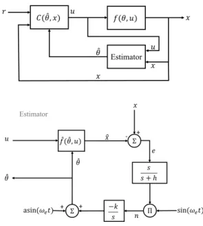
The typical structure of a control system with an estimator
is given in Fig. 1(a). The observer takes the controller
output, u, and the measured plant output, x, to estimate additional variables related to the plant. Dynamics of the plant is represented with function, f (θ, u, t). The controller, C, calculates its output based on the given setpoint, r,
measured output, x, and estimated output, ˆθ.
In order to operate the controller structure given in
Fig.1(a), a dependable observer algorithm that estimates the
unmeasured data, θ should be designed. In Fig.1(b), structure
of the proposed estimator is presented. The estimation uses the error, e, between the output of the plant, x, and the model
of the plant, ˆx to estimate the correct value of the unknown
2020 IEEE/ASME International Conference on Advanced Intelligent Mechatronics (AIM), Boston, USA (Virtual Conference), July 6-9, 2020
𝑓(𝜃, 𝑢) Estimator 𝑥 𝑢 𝑥 𝑢 (𝜃 𝐶( (𝜃, 𝑥) 𝑟 𝑥 (𝑓( (𝜃, 𝑢) 𝑥 𝑢 (𝜃 +𝑥 - + 𝑠 𝑠 + ℎ Π sin(𝜔!𝑡) −𝑘 𝑠 Σ Σ asin(𝜔!𝑡) + + 𝑒 (𝜃 Estimator 𝑛
Fig. 1: (a)Overview of the feedback control system with an estimator (b)Structure of the proposed Estimator
plant parameter, θ. Based on the error, the estimation of the
plant parameter, ˆθ, is updated at each loop using harmonic
modulation and shift parameters and signal conditioning.
The mechanism of the estimator given in Fig. 1(b) can
be explained following the stability and analysis method presented in [8]. Let’s assume that the output of the actual
plant, x, and the model of the plant, ˆx are calculated using
(1) and (2) respectively.
x = f (θ, u) (1)
ˆ
x = ˆf (ˆθ, u) (2)
where u is the controller command, θ is an unknown plant
parameter and ˆθ = θ + θd is the estimation of this unknown
plant parameter.
Based on the plant and model outputs, an estimation error, e, can be calculated as
e(θ, ˆθ, u) = f (θ, u) − ˆf (ˆθ, u) (3)
Let’s also assume that the error function given in (3) can be
written in the form:
e(θ, ˆθ, u) = g(θd)h(θ, θd, u) (4)
where g(θd) is a function with g(0) = 0 and g00 > 0. It is
also important to note that the error in estimation, e will be
minimized as long as the function g(θd) is zero while the
controller input, u is finite. An approximation to this function
can be written using the expansion given in (5).
g(θd) = g∗+
g00
2(θ
∗
d− θd)2 (5)
with θ∗d= 0 and g∗= 0. Then following Fig.1,
e = g
00
2(4θ − a sin(ωt))
2h(θ, θ
d, u) (6)
where 4θ = θ∗d−θd= −θd. Since the error function is given
in the factorized form, and minimized when g is minimized,
we can rewrite the error function as e = esh(θ, θd, u) and
concentrate on es.
Using the trigonometric property cos2ωt = cos2ωt −
sin2ωt = 1−2sin2ωt, one can obtain another approximation
for the output expression, as shown in (8).
es= ( g00 2 4 θ 2− ag00sinωt +a2g00 2 sin 2ωt) (7) es= ( a2g00 4 + g00 2 4 θ 2− ag004 θsinωt + a2g00 cosωt) (8)
Then applying the high-pass filter shown in Fig. 1 washes
out the slowly changing terms in (8) to obtain:
ef = s s + hes= ( g00 2 4 θ 2− ag00sinωt +a2g00 4 cos2ωt) (9)
After multiplication with sinωt and using well-known
trigonometric identities sin2ωt = 1/2 − cos2ωt/2 and
2cos2ωtsinωt = sin3ωt − sinωt we obtain the formulation
for the ζ signal given in Fig. 1as
n = −(ag 00 2 4 θ + ag00 2 4 θcos2ωt +a 2g00 8 (sinωt − sin3ωt) + f00 2 4 θ 2sinωt) (10)
Since 4θ = −θd, we also get 4 ˙θ = − ˙θd. Therefore as
the last calculation to complete the loop given in Fig. 1we
arrive at the expression for 4θ as shown in (11) by omitting
the quadratic term in 4θ.
4θ = k s(− ag00 2 4 θ + ag00 2 4 θcos2ωt +a 2g00 8 (sinωt − sin3ωt)) (11)
Then after disregarding the high frequency portion of (11)
due to integration, the final equation can be rewritten in the form
4 ˙θ ≈ −kag
00
2 4 θ (12)
Equation given in (12) implies a stable system when
kag00 > 0. This means as the system starts operating, the
estimator dynamics will drive 4θ to zero. This implies
θd = 0 and e = 0. Therefore the unknown plant variable,
θ, will be estimated and can be used by the controller for calculating the command action.
III. EXAMPLE: UNBALANCEDMASSPOSITION
ESTIMATION
In this section, an extremum seeking estimator described
in SectionIIwill be applied to a robotic device to improve its
locomotion performance. This device was developed as part of a research project, and it locomotes using the unbalanced mass force provided by a vibration motor embedded to its chassis. The details of the initial development on this device were presented in [9], [10], and [11]. Since the vibration motor is a closed component with no sensors, the initial
angular position of the unbalanced mass is not known once the device operates. In fact, due to its small mass, the unbalanced mass arm is also known to rotate without a command due to the effect of the impact forces.
A. Overview
The MechaCell prototype device, which developed as part of a manipulation testbed, is presented in [11] .MechaCells are planned as cheap but mighty devices used in groups. Each device has computing, actuation, and sensing capabilities with a wireless communication link.
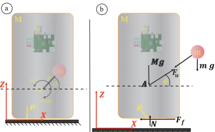
In Fig.2, the working principle of the locomotion system is
explained in four phases with respect to the unbalanced mass angular position. As the unbalanced mass fixed to the frame of the device rotates, it generates a centripetal force along with the link. Depending on the direction of the rotation, this force causes an accelerating and decelerating motion to the mainframe proportional to the rotation speed. Generally, during the full rotation of the unbalanced mass when π/2 ≤ θ ≤ 3π/2, the device stays still under the influence of the friction until it reaches phase I again.
Mathematical Model for MechaCell Dynamics
In Fig.2(a), a planar view of the system focusing on the
rotating unbalance motion is given with related parameters.
In Fig.2(b)a free body diagram of the system presented in
Figure (2(a)) is shown. Friction force acting on the system is
modeled by using Coulomb’s friction model with static and dynamic coefficients.
M M
m
a b
m
Fig. 2: (a) Planar Representation of the Rotating Unbalance (b) Free Body Diagram
Magnitude of the centripetal force, Fu, produced by the
rotating unbalance depends on the angular speed, ω, as
shown in (13)), the magnitude of the projections of the
centripetal force on X-axis and Z-axis are shown in (14))
and (15) respectively. In (16), the magnitude of the normal
force, N , as a function of ω is presented. Magnitude of the
friction force, Ff, as a function of ω is shown in Equation
(17). Fu(ω) = ω2mr (13) FuX(ω) = cos(θ)ω2mr (14) FuZ(ω) = sin(θ)ω2mr (15) N (ω) = M g − FuZ(ω) (16) Ff(ω) = −N (ω)µsign(v) (17)
After all of its components are identified, the equation that describes the motion of the device in the x-direction can be written as
FuX+ Ff = (M + m)aX (18)
where aX is the acceleration of the device in the
x’-direction. In Table (I) parameters, their symbols and units
used in the simulations are listed.
TABLE I: Numerical Values of the Parameters Used in the Mathematical Model
Parameter Symbol Value [unit]
Mass of the MechaCell M 0.049 [kg] Mass of the rotating unbalance m 0.006 [kg] Radius of the rotating unbalance r 0.004 [m] Coefficient of friction µ 0.2 [–] Force produced by the unbalance Fu calculated [N ]
Friction force Ff calculated [N ]
Normal force N calculated [N ]
Gravitational constant g 9.81 [m/s2]
Angular speed of the unbalance ω swept [rad/s]
Velocity v calculated [m/s]
B. Estimator Design
When equations given in (13)-(17) are investigated, one
can easily decide that unbalanced mass angular motion variable, θ, and its derivative, ω, are important to precisely calculate and control the generated locomotion force. The angular speed of the unbalanced mass is an input to the vi-bration motor and can be calculated using supplier provided constants. Calculating the position of the unbalanced mass, θ, can be complicated. Under ideal conditions, this variable can be calculated using
θ = θ0+
Z t
0
ω(t)dt (19)
where θ0is the initial position. By investigating the diagrams
shown in Fig. 2 the expected value of θ0 would be −90◦
due to gravity. However, due to the non-linear friction force, the initial value of the angle changes. Furthermore, even if the initial angle is somehow detected, due to its small inertia (4 grams), the position of the unbalanced mass may change abruptly during operation with impact forces due to contact with objects, etc. Therefore, estimation and continuous monitoring of the unbalanced mass position is necessary rather than merely integrating the speed command,
as shown in (19).
Using the proposed estimator idea from Section II an
error function can be defined based on the angular position mismatch of the plant and the model:
where aX = mω2r (M + m)(cos(θ) − (M g + µ sin(θ)) (21) aX,m= mω2r (M + m)(cos(θ +θd)−(M g +µ sin(θ +θd)) (22)
Using equations (21) and (22), the error equation in (20) can
be rewritten as
e = mω
2r
(M + m)(cos(θ) − cos(θ + θd) − sin(θ) + sin(θ + θd))
(23) By using trigonometric identities and manipulation, an
alter-native way to write the equation given in (23) can be written
as e = 2 sin(θd 2)(µsign(v) cos(θ+ θd 2)+sin(θ+ θd 2)) mω2r (M + m) (24)
The error function given in (24) can be written as a
multiplication of two functions as shown in (25) and (26).
g(θd) = sin( θd 2) (25) h(θ, θd, ω) = 2(µsign(v) cos(θ+ θd 2)+sin(θ+ θd 2)) mω2r (M + m) (26) It is important to note that, requirements reported in the
previous section, g(0) = 0 and g00 ≥ 0 for 0 ≤ θd ≤ π
is valid for g(θd) in (25).
C. Controller Design
A typical closed-loop control system structure for the locomotion of devices described in Fig. ?? is given in
Fig.3(a). In this setup, a closed-loop controller determines
the desired control command to be sent to the vibration motor (actuator) driver, the actuation controller receives this
command and calculate the desired angular velocity, ωdes, of
the unbalanced mass and calculates the corresponding pulse width modulation (PWM) signal. The actuation controller also outputs a polarity signal (1 or −1) based on the sign
of udesto determine the direction of the rotation. Details of
the calculations in the Actuation Control box is shown in
Fig.3(b).
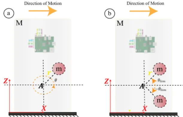
The actuation control approach explained before and given
in Fig.3(b) is titled as the ”Full Circle” actuation control
approach. In full circle actuation, the unbalanced mass com-pletes the full cycle with the commanded angular velocity,
ωdes, as shown in Fig.4(a). With the full circle rotation,
all the phases I-IV described in Fig.?? will be observed. However, an improvement to this operation can be made by operating the unbalanced mass only in the direction of motion by changing its polarity based on its position. With this new approach, the actuation system will operate in Phases I and IV, where the direction of the link force
is in the direction of the motion, as shown in Fig.4(b).
In this new approach the unbalanced mass moves in the
Actuator+Plant Dynamics 𝑢"!# 𝑥 Feedback Controller 𝑟"!# PWM Polarity (a) Typical Closed Loop Control
(b) Constant PWM Command 𝜔"!# 𝑢"!# 𝑚𝑟 𝑢"!# Polarity 𝑠𝑖𝑔𝑛(𝑢"!#)
Full Circle Actuation Control
Actuation Control
Actuation Control
Fig. 3: Typical Locomotion System Control Architecture
−θlim ≤ θ ≤ θlim range with the desired angular velocity,
ωdes. Because of the limits on the angular position, this
approach is named as the ”Limited Circle” actuation control approach. M a m M b m m
Direction of Motion Direction of Motion
Fig. 4: Full and Limited Unbalanced Mass Motion The ”limited circle” actuation approach described in the previous paragraph requires monitoring of the angular posi-tion of the unbalanced mass, θ, to switch the direcposi-tion of rotation when motion limits are reached. For small or cheap systems, a position sensor may not be readily available.
However, by using the estimator described in Section II, a
limited circle actuation algorithm can be implemented, as
shown in Fig.5.
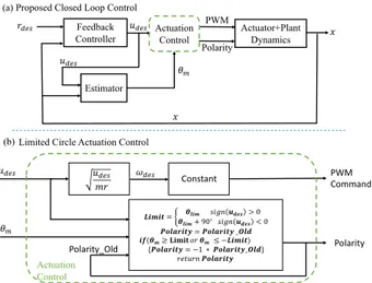
In Fig.5(a), the overall controller structure of the proposed
system is given. As compared to the original system given
in Fig.3(a), this proposed structure utilizes the estimator
shown in Fig. 1 to monitor the angular position, θm, of
the unbalanced mass. Based on the derivation described in
(1)-(26), the modeled angular position approaches to the
actual angular position once the system started. The modeled angular position is fed to the limited circle actuation control algorithm. In this algorithm, the angular velocity selection is
the same as the original approach given in Fig.3(b). However,
the polarity of the motor motion is flipped as the unbalanced mass position reaches its upper and lower limits based on the estimated angular position obtained from the estimator.
Actuator+Plant Dynamics 𝑢"!# 𝑥 Feedback Controller 𝑟"!# PWM Polarity Estimator 𝑥 𝜃$ 𝑢"!# PWM Command 𝜔"!# Constant Polarity 𝑢"!# 𝑢"!# 𝑚𝑟 𝜃$ 𝑳𝒊𝒎𝒊𝒕 = & 𝜽𝒍𝒊𝒎 𝑠𝑖𝑔𝑛 𝒖𝒅𝒆𝒔> 0 𝜽𝒍𝒊𝒎+ 90∘𝑠𝑖𝑔𝑛 𝒖𝒅𝒆𝒔< 0 𝑷𝒐𝒍𝒂𝒓𝒊𝒕𝒚 = 𝑷𝒐𝒍𝒂𝒓𝒊𝒕𝒚 _𝑶𝒍𝒅 𝒊𝒇(𝜽𝒎≥ 𝐋𝐢𝐦𝐢𝐭 𝑜𝑟 𝜽𝒎≤ −𝑳𝒊𝒎𝒊𝒕) {𝑷𝒐𝒍𝒂𝒓𝒊𝒕𝒚 = −1 ∗ 𝑷𝒐𝒍𝒂𝒓𝒊𝒕𝒚_𝑶𝒍𝒅} 𝑟𝑒𝑡𝑢𝑟𝑛 𝑷𝒐𝒍𝒂𝒓𝒊𝒕𝒚 Polarity_Old Limited Circle Actuation Control
Actuation Control
(a) Proposed Closed Loop Control
(b)
Actuation Control
Fig. 5: Proposed Locomotion System Control Architecture
The details of this algorithm are given in Fig.5(b).
IV. VALIDATION
In order to validate the ideas outlined in the previous sec-tions, both simulation and testbed experiments are performed using various settings. The validation work is divided into two parts. In the first part, the validity of the estimator is tested using different conditions. In the second part, this estimation algorithm is implemented as part of the limited circle actuation algorithm to validate its use for locomotion algorithms. In both cases, open-loop control, i.e., constant motor input, is used to separate the estimator and actuation control algorithm from the closed-loop control dynamics. A. Estimation Simulations
In order to validate the estimator presented in Fig. 1, a
MATLAB/Simulink model of the system presented in (13
)-(19) was developed. While running these simulations, the
real plant model is assumed to have an offset θd angle at
the beginning, which the estimator tries to estimate. The
estimator presented in Fig.1 is used with values a = 0.1,
ωe = 5000, h = 100 and k = {5, 10, 20} with the model
parameters presented in Table I. As discussed earlier, an
open-loop constant udes command that corresponds to the
mid-range of the PWM signal (P W M = 150) was used during the simulations.
In Fig.6, the effect of estimation gain k on the estimator
performance is shown. As predicted by (12), the increased
value of k decreases the time it takes to reach an estimation. However, as shown in the figure, the magnitude of high-frequency oscillations also increases with increased k. For all cases of k = {5, 10, 20} the estimator finds the correct
value of angle offset under 2s with estimation error θ − θm
approach to 0.
For many estimation problems, the magnitude of param-eter offset is also important to measure performance. If the parameter estimation does not converge to a value or converges to a wrong estimation, it can create problems. In order to measure the converging performance, various
0 0.5 1 1.5 2 2.5 3 3.5 4 4.5 5 Time [s] -20 -10 0 10 20 30 40 50 60 -m k=5 k=10 k=20 0 0.5 1 1.5 2 2.5 3 3.5 4 4.5 5 Time [s] -20 -10 0 10 20 30 40 50 60 d Estimated k=5 k=10 k=20 d
Fig. 6: Estimation using different gain, k values
theta offset values, i.e., θd is used to run simulations with
k = 10, and the estimated value of θd was recorded. The
results are shown in Fig. 7 for values of θd ranging from
0 to 90 degrees. As expected, from (25), the range of these
values is convergent and generates a correct estimation once the simulation starts. Since the value of estimator gain is
constant larger θd values require a longer time to reach a
steady value. 0 0.5 1 1.5 2 2.5 3 3.5 4 4.5 5 Time [s] -20 0 20 40 60 80 100 d Estimated d =15 d=30 d=45 d=60 d=90 X 2.7869 Y 15.651
Fig. 7: Estimation starting from differrent initial offset θd
using k = 10
B. Actuation Control
Results shown in both Fig.6 and Fig.7 are encouraging
enough to implement this estimation algorithm as part of the limited circle actuation control algorithm presented in
SectionIII-C. The same estimator settings from the previous
section are used with the same open-loop control udes.
First, the implementation of the estimator and the limited circle actuator was tested in the simulation environment. The motion circle for the unbalanced mass was limited to
θ = [−80, 80] degrees by setting θlim = 80. In order
to compare the results, full circle actuation with the same
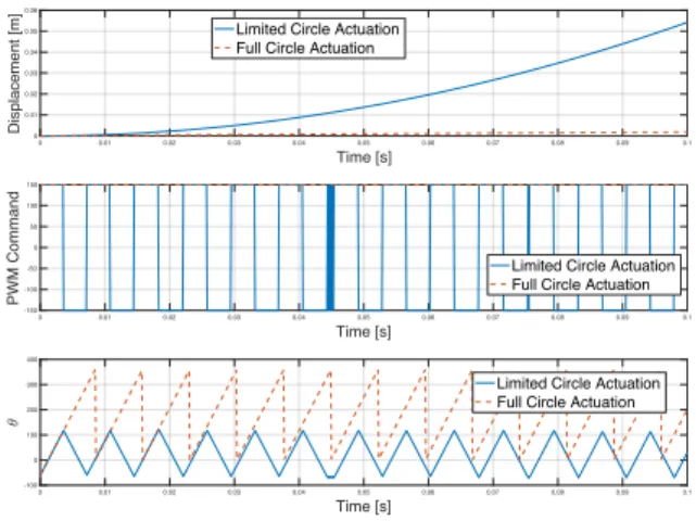
constant command was also run. Fig. 8 shows the results
obtained using simulations. The results in the figure show the theoretical benefit of limiting the motion cycle in this application. Since our model does not have any digital
effects and no actuator dynamics, the device locomotes as conceptualized with great acceleration as compared to the full circle alternative.
0 0.01 0.02 0.03 0.04 0.05 0.06 0.07 0.08 0.09 0.1 Time [s] 0 0.01 0.02 0.03 0.04 0.05 0.06 Displacement [m]
Limited Circle Actuation Full Circle Actuation
0 0.01 0.02 0.03 0.04 0.05 0.06 0.07 0.08 0.09 0.1 Time [s] -150 -100 -50 0 50 100 150 PWM Command
Limited Circle Actuation Full Circle Actuation
0 0.01 0.02 0.03 0.04 0.05 0.06 0.07 0.08 0.09 0.1 Time [s] -100 0 100 200 300 400
Limited Circle Actuation Full Circle Actuation
Fig. 8: Estimation using different gain, k values
The testbed experiments shown in Fig.9 show a more
realistic and also successful result set. In order to operate the
system, the ωe value was reduced to 1000, and data points
were taken at a rate of 10ms due to digital implementation
limitations. The PWM plot in Fig.9show that the signal was
switched successfully at estimated θ limits, and the device is displaced almost 5 times more than the full circle result with the same command. This improvement is overall an improvement on the locomotion system of the device with the use of only algorithms and no additional sensor to include.
0 0.1 0.2 0.3 0.4 0.5 0.6 0.7 0.8 0.9 1 Time [s] 0 0.02 0.04 0.06 0.08 0.1 Displacement [m]
Limited Circle Actuation Full Circle Actuation
0 0.1 0.2 0.3 0.4 0.5 0.6 0.7 0.8 0.9 1 Time [s] -150 -100 -50 0 50 100 150 PWM Command
Limited Circle Actuation Full Circle Actuation
0 0.1 0.2 0.3 0.4 0.5 0.6 0.7 0.8 0.9 1 Time [s] -100 0 100 200 300 400 Estimated
Limited Circle Actuation Full Circle Actuation
Fig. 9: Estimation using different gain, k values During validation simulations and experiments few chal-lenges related to the wide use of this method in its current form also aroused. In order to obtain a high fidelity error function for the estimator, the sampling rate needs to be appropriate. This means the sampling rate should be suitable for the dynamics generated by the unbalanced mass angular speed, which is the controller input in this example. Changes
in the frequency content of the error function may also require to change the estimator sinusoidal functions in order to obtain convergence. In this example, the performance of the estimator was optimized using a mid value controller input. The maximum speed of the vibration motor is given around 1500rpm. Therefore the estimator was designed for a speed of 750rpm.
V. CONCLUSIONS
In this paper, a new estimation technique based on ex-tremum seeking is presented. The method utilizes the idea of minimization of a non-linear error function of a certain form, which may be suitable for systems with periodic dynamics such as systems with unbalanced masses. This proposed method then applied to a mobile robotic system to improve its locomotion. Our initial results showed promising improvements up to five times more displacement with the same command on a testbed environment. Our future work includes estimating more variables, application to closed-loop control systems, and better handling digitization and power electronics to accommodate high frequency dynamics.
ACKNOWLEDGMENTS
Research supported by European Commission through Seventh Framework Program for Research and Technological Development under the contract PIRG07-GA-2010-268420.
REFERENCES
[1] M. Iwasaki, T. Shibata, and N. Matsui, “Disturbance-observer-based nonlinear friction compensation in table drive system,” IEEE/ASME Transactions on Mechatronics, vol. 4, pp. 3–8, mar 1999.
[2] Z. Zhang and S. Xu, “Observer design for uncertain nonlinear systems with unmodeled dynamics,” Automatica, vol. 51, pp. 80–84, jan 2015. [3] H. Cao, T. D¨orgeloh, O. Riemer, and E. Brinksmeier, “Adaptive Separation of Unbalance Vibration in Air Bearing Spindles,” Procedia CIRP, vol. 62, pp. 357–362, 2017.
[4] K. T. Atta, A. Johansson, and T. Gustafsson, “Extremum seeking control based on phasor estimation,” Systems & Control Letters, vol. 85, pp. 37–45, nov 2015.
[5] D. Nesic, A. Mohammadi, and C. Manzie, “A Framework for Ex-tremum Seeking Control of Systems With Parameter Uncertainties,” IEEE Transactions on Automatic Control, vol. 58, pp. 435–448, feb 2013.
[6] M. Xia and M. Benosman, “Extremum seeking-based indirect adaptive control for nonlinear systems with time-varying uncertainties,” in 2015 European Control Conference (ECC), pp. 2780–2785, IEEE, jul 2015. [7] G. Lara-Cisneros, D. Dochain, and J. Alvarez-Ram´ırez, “Model based extremum-seeking controller via modelling-error compensation ap-proach,” Journal of Process Control, vol. 80, pp. 193–201, aug 2019. [8] K. B. Ariyur and M. Krstic, Real time optimization by extremum
seeking control. Wiley Interscience, 2003.
[9] S. Ristevski and M. C¸ akmakcı, “Mathematical Model for Coordinated Motion of Modular Mechatronic Devices (MechaCells),” in Volume 2: Diagnostics and Detection; Drilling; Dynamics and Control of Wind Energy Systems; Energy Harvesting; Estimation and Identi-fication; Flexible and Smart Structure Control; Fuels Cells/Energy Storage; Human Robot Interaction; HVAC Building Energy M, p. V002T34A010, American Society of Mechanical Engineers, oct 2015.
[10] S. Ristevski and M. Cakmakci, “Mechanical design and position control of a modular mechatronic device (MechaCell),” in 2015 IEEE International Conference on Advanced Intelligent Mechatronics (AIM), vol. August, pp. 725–730, IEEE, jul 2015.
[11] S. Ristevski and M. Cakmakci, “Planar motion controller design for a modular mechatronic device with heading compensation,” Mechatron-ics, vol. 62, p. 102257, oct 2019.