NEW KEYNESIAN SMALL OPEN ECONOMY: TURKISH CASE
A Master’s Thesis by SEDAT ERSOY Department of Economicsİhsan Doğramacı Bilkent University Ankara
NEW KEYNESIAN SMALL OPEN ECONOMY: TURKISH CASE
The Institute of Economics and Social Sciences
of
İhsan Doğramacı Bilkent University
By
SEDAT ERSOY
In Partial Fulfillment of the Requirements for the Degree
of
MASTER OF ARTS
in
THE DEPARTMENT OF
ECONOMICS
İHSAN DOĞRAMACI BILKENT UNIVERSITY
ANKARA
iii
ABSTRACT
NEW KEYNESIAN SMALL OPEN ECONOMY: TURKISH CASE
ERSOY, SedatM.A, Department of Economics
Supervisor: Assistant Prof. Dr. Sang Seok Lee June 2016
Turkey experienced substantial declines in inflation after 2002. Was it due to good policy, good luck, or both? To address this question, we incorporate stochastic volatility into a small open new Keynesian model of Monacelli (2005). As demonstrated by Fernandez-Villaverde, Guerron-Quintana, Rubio-Ramirez (2010), volatility shocks are an importance source of macroeconomic fluctuations so they need to be accounted for in order to examine the good luck hypothesis rigorously. Our estimated model suggests that both good policy and good luck played roles in bringing down the inflation.
Keywords: Incomplete pass-through of exchange rate, Particle filter, Pruning, Stochastic Volatility
iv
ÖZET
DIŞA AÇIK KÜÇÜK EKONOMİ İÇİN YENİ KEYNESYEN
MODEL: TÜRKİYE OLAYI
ERSOY, Sedat
Yüksek Lisans, Ekonomi Bölümü Tez Yöneticisi: Yrd. Doç. Dr. Sang Seok Lee
Haziran 2016
Türkiye’nin 2002 yılından sonraki enflasyon oranlarında çok ciddi bir azalma görülmektedir. Sebebi iyi politika mıdır, iyi şans mıdır yoksa her ikisinin sonucunda mı oluşmuştur? Bu soruya cevap bulabilmek için Monacelli (2005) te ki Yeni Keynesyen dışa açık küçük ekonomi modeline stokastik volatilite eklenilmiştir. Fernandez-Villaverde, Guerron-Quintana, Rubio-Ramirez (2010) da gösterildiği gibi, stokastik volatilite makroekonomik dalgalanmaları açıklamada önemli bir kaynak, bu yüzden iyi şans hipotezimizi incelerken dikkate alınıp modele eklenmiştir. Türkiye verisiyle tahmin edilmiş modelimiz iddia ediyor ki; enflasyon oranlarının bu denli düşmesinde hem iyi politika hem de iyi şans rol almıştır.
Anahtar Kelimeler: Budama, Eksik Döviz Yansıması, Partikül Filtresi, Stokastik Volatilite
v
ACKNOWLEDGEMENTS
I would like to express my cordial gratitude to my supervisor Asst. Prof. Sang Seok Lee for his exceptional supervision, academic guidance, and continuous support through my thesis. It was a great chance and honor for me to study under his invaluable guidance. I would also like to thank to Assoc. Prof. H. Çağrı Sağlam and Asst. Prof. Ö. Kağan Parmaksız for their valuable comments on my thesis.
I am grateful to Prof. Semih Koray, Prof. Refet S. Gürkaynak, and Assoc. Prof. Emin Karagözoğlu for their support during the master’s program.
I would also like to thank all T.A’s in Department of Economics, İ.D. Bilkent University for their help through two years of graduate school. In particular, I am grateful to Erion Dula and Ömer Faruk Akbal for their continuous and endless support, and sincere friendship.
I would also like to thank TÜBİTAK for their financial support during my graduate years.
I am grateful to my family for their love and support. Last but not least, the most special thanks go to my wife Büşra. This accomplishment could not have been possible without her endless support, encouragement, and affection.
vi
TABLE OF CONTENTS
ABSTRACT……….iii ÖZET………....iv ACKNOWLEDGEMENT………...v TABLE OF CONTENTS………....vi LIST OF TABLES………viii LIST OF FIGURES………...ix CHAPTER 1: INTRODUCTION……….………...1CHAPTER 2: THE MODEL………...3
2.1 Households……….3
2.2 Firms………...9
2.3 Monetary Policy………….………...……14
CHAPTER 3: ESTIMATION RESULTS…….………...…16
3.1 Data…….……….………16
3.2 Estimation Results...……….16
CHAPTER 4: SOLUTION AND DYNAMICS…...………21
vii
4.2 Dynamics..………22
4.3 Evolution of the Taylor Rule Parameter for Inflation ……….28
CHAPTER 5: CONCLUSION………..32
viii
LIST OF TABLES
1. Particle Filter Estimation Results……….………18
2. Calibrated Values……….………19
ix
LIST OF FIGURES
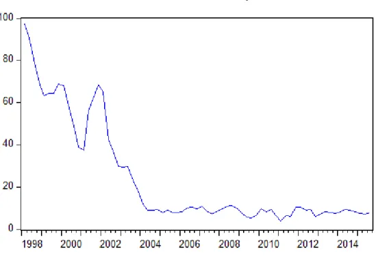
1. Inflation Rate in Turkey………..2
2. The Impulse Response Functions to a Monetary Policy Shock (PF)………23
3. The Impulse Response Functions to a Monetary Policy Volatility Shock (PF)………24
4. The Impulse Response Functions to a Taylor Rule parameter for the Inflation (PF)……….………...25
5. The Impulse Response Functions to a Taylor Rule parameter for the Change in the Output Level (PF)……….25
6. The Impulse Response Functions to a TFP Shock (PF)………26
7. The Impulse Response Functions to a TFP Shock (KF)……….…..26
8. The Impulse Response Functions to a LOP Gap Shock (PF)………...27
9. The Impulse Response Functions to a LOP Gap Shock (KF)………...27
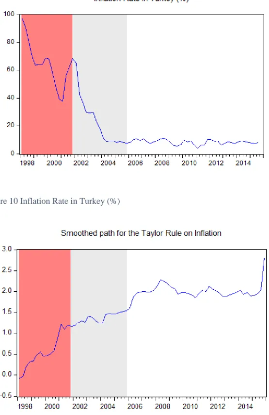
10. Inflation Rate in Turkey (%)……….……29
11. Smoothed Path for the Taylor Rule Parameter on Inflation……….……….29
1
CHAPTER 1
INTRODUCTIONWhen we look at the inflation rate in Turkey between 1998-2015 (see Figure 1) we have observed that there is a huge inflation rate before 2002, and it sharply goes down after 2002 and mostly have a single digit inflation rate after 2006. Interestingly the period between 2002 and 2005 corresponds to the implicit inflation targeting period in Turkey. After 2006 Turkey has an explicit inflation targeting and the main objective of the Central Bank of Turkey became to achieve and maintain price stability. As stated in Kara and Orak (2008) inflation targeting become successful in Turkey and Turkey has reached more stabilized price levels. At that point, we need to ask the following question: Even though many reforms and actions done in Turkey such as inflation targeting, establishing the Bank Regulatory and Supervisory Board, etc., might there be some possibilities of good luck in the economy in order to account for some part of the decline in inflation in Turkey? Or does all this success come from good policy? In order to answer this crucial question for Turkey case, we first build a nonlinear dynamic stochastic general equilibrium (DSGE) model, and then estimate the model parameters using Turkish data and accordingly solve the model so as to observe the dynamics of the Turkish economy. Hence, the rest of the paper follows as; in chapter 2 we will explain our model carefully, in chapter 3 using four
2
time series data we will do nonlinear estimation, and then using those estimated parameters we try to account for especially the changes in the inflation rate in Turkey. In chapter 4, we analyze the dynamics of the model. In chapter 5, we briefly conclude this project by mentioning our main findings and contributions to the literature and how we can go further in this project and what else can we do as a future research.
3 CHAPTER 2
THE MODEL
In this setup, following Monacelli (2005) closely we have just two countries which are home and foreign1. Home country is a small open economy and foreign country is the rest of the world. Small economy has no effect on the foreign economy because it is negligibly small compared to the rest of the world, hence it is assumed that variables in the foreign economy is exogenously determined. We will see in the next sections that foreign country has only one possible way to have an impact on small open economy which is just the foreign aggregate price level and foreign aggregate consumption level, hence we will focus on only the dynamics of the small open economy.
2.1) HOUSEHOLDS
One of the main actors in our model is households. There is a continuum of them located between 0 and 1, i.e. each individuals are indexed by k and k∈ [0, 1], and by doing so its mass is normalized to 1. However, we assume that there is a representative household in this economy so we can drop the k index. Representative household gets utility from consumption and disutility from number of hours worked, so we can express their life time utility which is separable in both consumption and number of hours labor as the following;
4 𝐸0{∑ 𝛽𝑡(𝐶𝑡 1−𝜎 1 − 𝜎− 𝑁𝑡1+𝜑 1 + 𝜑) ∞ 𝑡=0 } (1)
where β is the discount factor, σ is the inverse elasticity of intertemporal substitution, φ is the inverse elasticity of labor supply. Nt denotes hours of labor, Ct denotes consumption
index of foreign and domestically produced goods which can be defined as:
𝐶𝑡 = ((1 − 𝛼) 1 𝜂𝐶 ℎ,𝑡 𝜂−1 𝜂 + 𝛼 1 𝜂𝐶 𝑓,𝑡 𝜂−1 𝜂 ) 𝜂 𝜂−1 (2)
where α ∈ [0, 1] is the degree of openness for the domestic country, η > 0 is the elasticity of substitution between domestic and foreign goods. The aggregate consumption indices of domestically and foreign produced goods can be defined respectively as:
𝐶ℎ,𝑡 = (∫ 𝐶ℎ,𝑡(𝑖)𝜀−1𝜀 1 0 𝑑𝑖) 𝜀 𝜀−1 (3) 𝐶𝑓,𝑡 = (∫ 𝐶𝑓,𝑡(𝑖)𝜀−1𝜀 1 0 𝑑𝑖) 𝜀 𝜀−1 (4)
Above indexes are valid under the assumption that there are infinitely many goods indexed by i∈ [0, 1], and ε > 1 which is the elasticity of substitution between varieties of goods. Ch,t(i) is the consumption of domestic good i by domestic household at time t, similarly
Cf,t(i) denotes the consumption of foreign good i by domestic household at time t. In this
model representative household faces two problems which are expenditure minimization and maximization of the expected life time utility.
At any point in time they have expenditure in both domestically produced goods and foreign produced goods, so their total expenditure will be the following;
5
∫(𝑃ℎ,𝑡(𝑖)𝐶ℎ,𝑡(𝑖) + 𝑃𝑓,𝑡(𝑖)𝐶𝑓,𝑡(𝑖))𝑑𝑖 1
0
Then representative household will minimize their expenditure subject to (3).
ℒ = ∫ (𝑃ℎ,𝑡(𝑖)𝐶ℎ,𝑡(𝑖) + 𝑃𝑓,𝑡(𝑖)𝐶𝑓,𝑡(𝑖)) 𝑑𝑖 + 𝜆1,𝑡 ( 𝐶ℎ,𝑡 − (∫ 𝐶ℎ,𝑡(𝑖) 𝜀−1 𝜀 𝑑𝑖 1 0 ) 𝜀 𝜀−1 ) 1 0 + 𝜆2,𝑡 ( 𝐶𝑓,𝑡− (∫ 𝐶𝑓,𝑡(𝑖) 𝜀−1 𝜀 1 0 𝑑𝑖) 𝜀 𝜀−1 )
FOC with respect to Ch,t(i) will give the following condition;
𝑃ℎ,𝑡(𝑖) − 𝜆1,𝑡𝐶ℎ,𝑡 1 𝜀𝐶ℎ,𝑡(𝑖)− 1 𝜀 = 0 ⇒ 𝐶ℎ,𝑡(𝑖) = ( 𝑃ℎ,𝑡(𝑖) 𝜆1,𝑡 ) −𝜀 𝐶ℎ,𝑡 (5)
Here, we find inverse demand function for each domestically produced goods i, but the form can be rewritten in more elegant version because we do not have an idea about λ1,t.
Put equation (5) into (4), then λ1,t can be obtained as
𝑃ℎ,𝑡 ∶= 𝜆1,𝑡 = (∫ 𝑃ℎ,𝑡(𝑖)1−𝜀𝑑𝑖 1 0 ) 1 1−𝜀 (6)
where Ph.t is the price index of domestically produced goods. Now equation (5) can be
expressed as
𝐶ℎ,𝑡(𝑖) = (𝑃ℎ,𝑡(𝑖) 𝑃ℎ,𝑡 )
−𝜀
𝐶ℎ,𝑡 (7)
By symmetry we can also define price index of foreign produced goods and by using it we can obtain inverse demand function for each foreign produced goods.
6 𝑃𝑓,𝑡 ∶= 𝜆2,𝑡 = (∫ 𝑃𝑓,𝑡(𝑖)1−𝜀𝑑𝑖 1 0 ) 1 1−𝜀 𝐶𝑓,𝑡(𝑖) = (𝑃𝑓,𝑡(𝑖) 𝑃𝑓,𝑡 ) −𝜀 𝐶𝑓,𝑡 (8)
If we use equation (7) and equation (8) respectively, we have the following forms
∫ (𝑃ℎ,𝑡(𝑖)𝐶ℎ,𝑡(𝑖)) 𝑑𝑖 1 0 = 𝑃ℎ,𝑡𝐶ℎ,𝑡 ∫ (𝑃𝑓,𝑡(𝑖)𝐶𝑓,𝑡(𝑖)) 𝑑𝑖 1 0 = 𝑃𝑓,𝑡𝐶𝑓,𝑡
So in aggregate indexes total expenditure function can be rewritten as
∫(𝑃ℎ,𝑡(𝑖)𝐶ℎ,𝑡(𝑖) + 𝑃𝑓,𝑡(𝑖)𝐶𝑓,𝑡(𝑖))𝑑𝑖 1
0
= 𝑃ℎ,𝑡𝐶ℎ,𝑡+ 𝑃𝑓,𝑡𝐶𝑓,𝑡 (9)
Since we express all the variables without index i, equivalently we can minimize total expenditure function subject to equation (2). From the FOC conditions, and using the same tricks used as in above case we have;
𝐶ℎ,𝑡 = (1 − 𝛼) (𝑃ℎ,𝑡 𝑃𝑡 ) −𝜂 𝐶𝑡 (10) 𝐶𝑓,𝑡 = 𝛼 (𝑃𝑓,𝑡 𝑃𝑡) −𝜂 𝐶𝑡 (11)
Now if we combine equations (10) and (11) with the right hand side of the equation (9), we have;
7
𝑃ℎ,𝑡𝐶ℎ,𝑡+ 𝑃𝑓,𝑡𝐶𝑓,𝑡 = 𝑃𝑡𝐶𝑡 (12)
where 𝑃𝑡: = ((1 − 𝛼)𝑃ℎ,𝑡1−𝜂 + 𝛼𝑃𝑓,𝑡1−𝜂)
1 1−𝜂
can be defined as overall consumer price index. So in our model CPI (consumer price index) and the price index of domestically produced goods are differentiated.
Representative household has expenditure due to consumed goods, and holding financial portfolio, and getting wage due to number of labor she supplies, hence she has the following budget constraint;
𝑃𝑡𝐶𝑡+ 𝐸𝑡{𝑄𝑡,𝑡+1𝐷𝑡+1} = 𝐷𝑡+ 𝑊𝑡𝑁𝑡 (13)
where Qt,t+1 is the stochastic discount factor, i.e. discounting the value of any variable at
t+1 to the value of it at t, and Dt+1 is the nominal payoff in t+1 of a financial portfolio held
in t. Actually when we discount it today, it will be equal to the price of this portfolio so that household pays this amount of money to get this portfolio. However, as of today she will get wage for each hour of labor supplied and she will get Dt nominal payoff of a
financial portfolio held in t-1. Hence we have the above budget constraint in t.
Representative household determines the level of Ct, Nt and Dt+1 at time t, so she will
maximize her life time discounted utility subject to (13) with respect to those variables. FOC with respect to Ct will give: 𝐶𝑡−𝜎 = 𝜆3,𝑡𝑃𝑡 and FOC with respect to Nt will give:
𝑁𝑡𝜑 = 𝜆3,𝑡𝑊𝑡 where 𝜆3,𝑡 is the Lagrange multiplier corresponding to budget constraint of the representative household. If we combine above two conditions and get rid of the 𝜆3,𝑡, we get the following intratemporal condition:
8 𝐶𝑡−𝜎
𝑁𝑡𝜑 = 𝑃𝑡
𝑊𝑡
This condition actually equates the marginal rate of substitution between consumption and hours of labor to the ratio of the prices of them respectively.
As stated by Schmitt-Grohe and Uribe (2003) small open economies with incomplete financial market has non-stationary dynamics because when there is no complete financial market, marginal utility will follow random walk as showed in Hall (1978) hence to make it stationary Schmitt-Grohe and Uribe (2003) proposes 5 different way to cope with this non-stationarity. For simplicity we choose the easiest option hence we assume that there is a complete financial market. Before obtaining the intertemporal FOC condition, we need more calculations. In the complete market, we have
𝑉𝑡,𝑡+1𝐶𝑡
−𝜎
𝑃𝑡 = 𝜉𝑡,𝑡+1𝛽 𝐶𝑡+1−𝜎 𝑃𝑡+1
where 𝑉𝑡,𝑡+1 is the domestic price of an Arrow security in t (i.e. when a specific state is realized in t+1, it is a one period security that yields one unit of home currency), and 𝜉𝑡,𝑡+1
is the probability of that state is realized. Here since we have complete financial market assumption we will have 𝑄𝑡,𝑡+1 = 𝑉𝑡,𝑡+1
𝜉𝑡,𝑡+1 , hence we can rewrite the above equality as
𝑄𝑡,𝑡+1 = 𝛽 𝑃𝑡 𝑃𝑡+1( 𝐶𝑡+1 𝐶𝑡 ) −𝜎
Compared to the incomplete market, this condition is satisfied for all possible states in t+1, instead this is satisfied only under the expectation operator in the incomplete market. However, since we know that gross return of a risk free nominal bond can be expressed
9 as 𝑅𝑡 = 1
𝐸𝑡{𝑄𝑡,𝑡+1} , after taking the expectation of the above expression it can be rewritten
as 𝛽𝑅𝑡𝐸𝑡{ 𝑃𝑡 𝑃𝑡+1 (𝐶𝑡+1 𝐶𝑡 ) −𝜎 } = 1
which is the Euler equation derived from intertemporal FOC. 2.2) Firms
There is a continuum of firms which are owned by households and indexed by j and they have linear production function 𝑌𝑡(𝑗) = 𝑍𝑡𝑁𝑡(𝑗) where 𝑌𝑡(𝑗)is the level of production by
firm j and 𝑁𝑡(𝑗) is the labor input of the firm j and 𝑍𝑡 is the total factor productivity (TFP)
which is same for all the firms. 𝑍𝑡 has stochastic AR(1) process2:
𝑍𝑡 = (1 − 𝜌𝑧) + 𝜌𝑧𝑍𝑡−1+ 𝜎𝑧,𝑡𝜉𝑧,𝑡
where 𝜉𝑧,𝑡∼N(0,0.01). As you can notice here, standard deviations 𝜎𝑧,𝑡 of the innovation 𝜉𝑧,𝑡 is not constant, and it evolves over time. Hence we add time varying stochastic
volatility to our model as in Fernandez-Villaverde, Guerron-Quintana, Rubio-Ramirez (2010) [FGR (2010) henceforth]. Now there is no unique way to express the evolution of 𝜎𝑧,𝑡, even it can follow Markov chain and takes different values for different states, but as FGR (2010) states this will make the estimation procedure harder because we need to use global solution methods instead of perturbation method, and estimation with global solution methods takes much more time than the estimation with perturbation method. Therefore, we closely follow FGR (2010), and 𝜎𝑧,𝑡 has an AR(1) process in logs:
2 Here we assume that Z
10
𝑙𝑜𝑔𝜎𝑧,𝑡 = (1 − 𝜌𝜎𝑧)𝑙𝑜𝑔𝜎𝑧+ 𝜌𝜎𝑧𝑙𝑜𝑔𝜎𝑧,𝑡−1+ 𝑈𝑧,𝑡 where 𝑈𝑧,𝑡∼N(0,1) , and 𝜎𝑧 is the steady state level of 𝜎𝑧,𝑡.
Since we are only interested in the symmetric equilibrium, we can drop the j index for the firms, hence we can say that there is a representative monopolistic firm. We assume that they are not able to change their prices each period, there is a Calvo (1983) pricing friction in such a way that 𝜃ℎ fraction of the firms cannot set their prices in the period t, where 𝜃ℎ ∈ [0, 1].
Firms in this model have both cost minimization problem and profit maximization problem under the Calvo pricing mechanism. The former can be written as:
min
𝑁𝑡
𝑊𝑡
𝑃ℎ,𝑡
𝑁𝑡+ 𝜆3,𝑡(𝑌𝑡− 𝑍𝑡𝑁𝑡)
The FOC is:
𝑀𝐶𝑡 ≔ 𝜆3,𝑡 =
𝑊𝑡 𝑃ℎ,𝑡𝑍𝑡
where 𝑀𝐶𝑡 is the real marginal cost of the firm and we can also define nominal marginal cost as 𝑀𝐶𝑡𝑛 ≔𝑊𝑡
𝑍𝑡.
Before stating the profit maximization problem let’s define stochastic discount factor3 between period t and period t+k:
3 Since we assume that firms are owned by households, we can use the same discount factor in the firm’s
11 𝑄𝑡,𝑡+𝑘= 𝛽𝑘 𝑃𝑡 𝑃𝑡+𝑘( 𝐶𝑡+𝑘 𝐶𝑡 ) −𝜎
Normally, from the goods market equilibrium it must be that 𝑌𝑡= 𝐶ℎ,𝑡 + 𝐶ℎ,𝑡⚹ where 𝐶ℎ,𝑡⚹ is the consumed level of domestic goods by foreign country. Since small open economy is so small compared to the foreign one we can assume that 𝐶ℎ,𝑡⚹ = 0, hence goods market equilibrium becomes 𝑌𝑡= 𝐶ℎ,𝑡.
Then, we can formulate the profit maximization problem as follows:
max 𝑃ℎ,𝑛𝑒𝑤,𝑡 𝐸𝑡{∑ 𝜃ℎ𝑘𝑄𝑡,𝑡+𝑘 ∞ 𝑘=0 [𝑃ℎ,𝑛𝑒𝑤,𝑡− 𝑀𝐶𝑡+𝑘𝑛 ]𝑌𝑡+𝑘} subject to 𝑌𝑡+𝑘 = ( 𝑃ℎ,𝑛𝑒𝑤,𝑡 𝑃ℎ,𝑡+𝑘) −𝜂 𝐶ℎ,𝑡+𝑘 Equivalently, we have: max 𝑃ℎ,𝑛𝑒𝑤,𝑡 𝐸𝑡{∑ 𝜃ℎ𝑘𝑄𝑡,𝑡+𝑘 ∞ 𝑘=0 [𝑃ℎ,𝑛𝑒𝑤,𝑡1−𝜂 − 𝑀𝐶𝑡+𝑘𝑛 𝑃ℎ,𝑛𝑒𝑤,𝑡−𝜂 ]𝑃ℎ,𝑡+𝑘𝜂 𝐶ℎ,𝑡+𝑘}
The FOC is:
𝐸𝑡{∑ 𝜃ℎ𝑘𝑄𝑡,𝑡+𝑘 ∞ 𝑘=0 [(1 − 𝜂)𝑃ℎ,𝑛𝑒𝑤,𝑡−𝜂 + 𝜂𝑀𝐶𝑡+𝑘𝑛 𝑃ℎ,𝑛𝑒𝑤,𝑡−𝜂−1 ]𝑃ℎ,𝑡+𝑘𝜂 𝐶ℎ,𝑡+𝑘} = 0 Then we have: 𝐸𝑡{∑ 𝜃ℎ𝑘𝑄𝑡,𝑡+𝑘 ∞ 𝑘=0 [(1 − 𝜂) + 𝜂𝑀𝐶𝑡+𝑘𝑛 𝑃ℎ,𝑛𝑒𝑤,𝑡−1 ]𝑌𝑡+𝑘} = 0
12 After some manipulations we have:
𝑃ℎ,𝑛𝑒𝑤,𝑡 = 𝜂 𝜂 − 1 𝐸𝑡{∑∞𝑘=0𝜃ℎ𝑘𝑄𝑡,𝑡+𝑘[𝑀𝐶𝑡+𝑘𝑛 ]𝑌 𝑡+𝑘} 𝐸𝑡{∑∞𝑘=0𝜃ℎ𝑘𝑄𝑡,𝑡+𝑘𝑌𝑡+𝑘}
Let the numerator and the denominator be respectively 𝑓𝑡1 and 𝑓 𝑡2 as 𝑓𝑡1 = 𝐸𝑡{∑ 𝜃ℎ𝑘𝑄𝑡,𝑡+𝑘 ∞ 𝑘=0 [𝑀𝐶𝑡+𝑘𝑛 ]𝑌 𝑡+𝑘} 𝑓𝑡2 = 𝐸𝑡{∑ 𝜃ℎ𝑘𝑄𝑡,𝑡+𝑘 ∞ 𝑘=0 𝑌𝑡+𝑘}
Now, we need to express these terms in recursive forms so after evaluating them for k=0, and some manipulations we have:
𝑓𝑡1 = 𝑊𝑡 𝑍𝑡 𝑌𝑡+ 𝛽𝜃ℎ𝐸𝑡{𝑓𝑡+1 1 𝑃𝑡 𝑃𝑡+1( 𝐶𝑡+1 𝐶𝑡 ) −𝜎 } 𝑓𝑡2 = 𝑌𝑡+ 𝛽𝜃ℎ𝐸𝑡{𝑓𝑡+12 𝑃𝑡 𝑃𝑡+1 (𝐶𝑡+1 𝐶𝑡 ) −𝜎 } 𝑃ℎ,𝑛𝑒𝑤,𝑡 = 𝜂 𝜂 − 1 𝑓𝑡1 𝑓𝑡2
At time t, 𝜃ℎ portion of the firms cannot reset their prices hence they will use the previous period’s prices, but (1 − 𝜃ℎ) portion will set their prices as 𝑃ℎ,𝑛𝑒𝑤,𝑡, so overall price level of domestic goods can be written as the geometric average of both these prices:
𝑃ℎ,𝑛𝑒𝑤,𝑡 = (𝜃ℎ𝑃ℎ,𝑡−11−𝜂 + (1 − 𝜃ℎ)𝑃ℎ,𝑛𝑒𝑤,𝑡1−𝜂 )
1 1−𝜂
13
In our model, we can define the nominal exchange rate 𝜖𝑡 as the amount of domestic currency per unit of foreign currency. Under the assumption of no arbitrage opportunity, any goods must be hold with the same price in all locations which is called law of one price (LOP, hereafter) hence it must be that 𝑃𝑓,𝑡(𝑖) = 𝜖𝑡𝑃𝑡⚹(𝑖) where 𝑃𝑡⚹(𝑖) is the price of
a foreign goods in foreign country for i ∈ [0, 1], after aggregating4 over goods i we have
LOP condition in aggregate levels 𝑃𝑓,𝑡 = 𝜖𝑡𝑃𝑡⚹. As stated in Monacelli (2005) that we
present incomplete exchange rate pass-through on import prices. For a small economy it is intuitive to add such rigidity because of the size of the domestic country. When there is no influence on the rest of the world, they cannot have a bargaining power over the imported goods. So we can say that LOP holds at the dock, but there will be price dispersion between the domestic price of the imported goods and foreign price of the foreign goods. Hence Monacelli (2005) introduces the LOP gap by:
𝜓𝑡 =
𝜖𝑡𝑃𝑡⚹ 𝑃𝑓,𝑡
If there is a complete exchange rate pass-through, then 𝜓𝑡 must be 1 and LOP will hold, so any deviation of 𝜓𝑡 from 1 can be interpreted as the LOP gap. Furthermore, we assume that LOP gap has a stochastic AR(1) process in levels5:
𝜓𝑡 = (1 − 𝜌𝑙) + 𝜌𝑙𝜓𝑡−1+ 𝜎𝑙,𝑡𝜉𝑙,𝑡
4 Here we assume that foreign economy has the identical preferences as home economy has, hence we
can aggregate over goods i properly.
5 Since we know that in the long run there will be complete exchange rate pass-through, LOP holds at the
14
where 𝜉𝑙,𝑡∼N(0,0.01). Again as in the total factor productivity, standard deviations 𝜎𝑙,𝑡 of the innovation 𝜉𝑙,𝑡 is not constant, and it evolves over time. Hence we assume that 𝜎𝑙,𝑡 has an AR(1) process in logs:
𝑙𝑜𝑔𝜎𝑙,𝑡 = (1 − 𝜌𝜎𝑙)𝑙𝑜𝑔𝜎𝑙+ 𝜌𝜎𝑙𝑙𝑜𝑔𝜎𝑙,𝑡−1+ 𝑈𝑙,𝑡
where 𝑈𝑙,𝑡∼N(0,1) , and 𝜎𝑙 is the steady state level of 𝜎𝑙,𝑡.
2.3.) MONETARY POLICY
Monetary policy follows the modified Taylor rule as in FGR (2010):
log𝑅𝑡
𝑅 = 𝜌𝑟log 𝑅𝑡−1
𝑅 + (1 − 𝜌𝑟)[𝜃𝜋,𝑡log 𝜋𝑡+ 𝜃𝑦,𝑡(log 𝑌𝑡− log 𝑌𝑡−1)] + 𝜎𝑟,𝑡𝜉𝑟,𝑡 where 𝑅 is the steady state level of the gross rate of return, 𝜌𝑟 is the interest rate smoothing
parameter, 𝜃𝜋,𝑡 is the response to change in the price level, 𝜃𝑦,𝑡 is the response to change in the output level, and 𝜉𝑟,𝑡∼N(0,0.01). They called it modified Taylor rule because in the
simple policy rule 𝜃𝜋,𝑡 and 𝜃𝑦,𝑡 are constant, but in our case just like in FGR (2010) they evolve over time. The reasoning behind this is the following; the members of the monetary policy committee can change or their belief about the economy can change over time, so the overall reaction of the committee for inflation and change in the output level can be different, hence we assume that they have also AR(1) process in logs6:
log 𝜃𝜋,𝑡 = (1 − 𝜌𝜃𝜋) log 𝜃𝜋 + 𝜌𝜃𝜋log 𝜃𝜋,𝑡−1+ 𝜉𝜋,𝑡
6 Here assuming AR(1) process in logs we restrict ourselves to have positive values for Taylor rule
parameters, because it is not intuitive to have non-positive values for these parameters. As a future research we can consider the cases where these might be non-positive values too.
15
log 𝜃𝑦,𝑡 = (1 − 𝜌𝜃𝑦) log 𝜃𝑦+ 𝜌𝜃𝑦log 𝜃𝑦,𝑡−1+ 𝜉𝑦,𝑡
where |𝜌𝜃𝜋| < 1, and |𝜌𝑦| < 1, 𝜉𝜋,𝑡∼N(0,0.01), 𝜉𝑦,𝑡∼N(0,0.01), and 𝜃𝜋 and 𝜃𝑦 are the steady state levels of the 𝜃𝜋,𝑡 and 𝜃𝑦,𝑡 respectively.
We also introduce the time varying volatility for standard deviations of the monetary policy shock:
𝑙𝑜𝑔𝜎𝑟,𝑡 = (1 − 𝜌𝜎𝑟)𝑙𝑜𝑔𝜎𝑟+ 𝜌𝜎𝑟𝑙𝑜𝑔𝜎𝑟,𝑡−1+ 𝑈𝑟,𝑡
16 CHAPTER 3
ESTIMATION RESULTS
3.1) Data
In order to estimate our model, we use four time series covering the period 1998Q1-2015Q3 for Turkish economy. There are no a priori grounds to suspect trend components in these series so I take them to my detrended model. We use the following variables as observable: (i) the growth rate of the real GDP7, (ii) inflation rate by using the consumer price index (CPI), (iii) nominal exchange rate, and (iv) short term policy interest rate. 3.2) Estimation
Most of the literature linearize the model, and estimate their model with Kalman filter because Kalman filter is optimal when the shocks have Gaussian distribution and the model is linear8. Linear model is required because when it is so, the solution of the model can be written linearly. Hence linear combination of independent Gaussian distributions will again be Gaussian distribution and Kalman filter will be optimal in that case. However, we have a non-linear transition and a non-linear policy function, hence we use
7 Firstly, we try to use the output gap instead of the growth rate of the real GDP, but after we use HP filter
to get rid of the trend component and to obtain output gap, we faced so negative values for this variables and it makes us get in trouble in the estimation part, hence instead we used the growth rate of the real GDP as an observable.
8 Even though we have Gaussian distributed error terms, we cannot use Kalman filter because of the
17
particle filter estimation9 as done in FGR (2010). If there are more observables than the
shocks in the model, then it will cause stochastic singularity. To cope with this situation, measurement errors can be used10. However, in our case we have more than 4 shocks, so no need to worry about it. Due to the curse of dimensionality we have to reduce the number of the parameters to be estimated. We calibrate the following parameters as in the Monacelli (2005): α, η, 𝜑, 𝜎, 𝜃ℎ . The only exception is in the discount factor, we set11
𝛽 = 0.92.
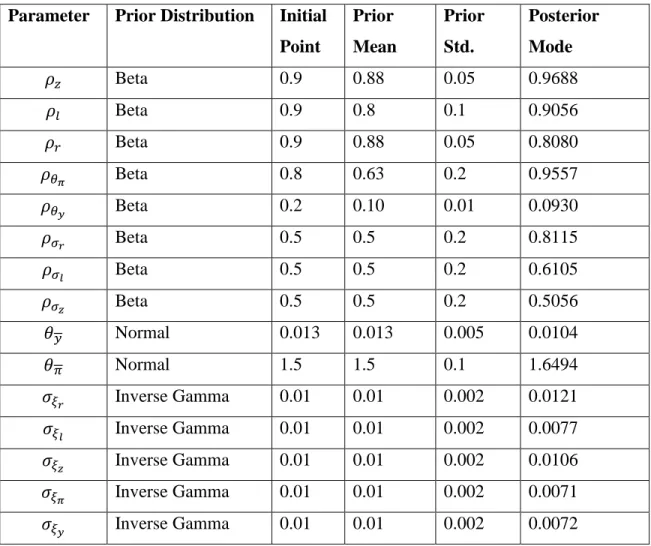
In order to estimate the model with particle filter, we should first propose valid priors for the parameters to be estimated. As stated in Sims (2014), it is quite common in the literature to use beta distributions for the parameters range between 0 and 1, and to use inverse gamma distributions for shock standard deviations and to use normal distributions for the other parameters. Hence we set our parameters accordingly. In the first column of the table12 1, we have the names of the parameters that we try to estimate, in the second column, we have the type of the distributions of the parameters, in the third column we assign some reasonable initial values for each of these parameters, in the fourth and the fifth column we determine the mean and standard deviations of these parameters, respectively. Lastly in the sixth column, we have the estimated mode values of these parameters after we use the particle filter. At first sight, we can say that Turkey has a quite
9 For an illustrative example for how the particle filter works, you can check Fernandez-Villaverde,
Rubio-Ramirez (2004).
10 We know that aggregate variables are calculated with big measurement errors, but we did not add the
measurement shocks for the observables since we have already 8 shocks in our model and adding 4 more shocks will affect the duration of the estimation part.
11 Otherwise with the previous value of discount factor particle filter does not work since the data and the
model does not match properly. Actually, the steady state level of the gross interest rate is equal to 1/β, and we know that historical values of gross interest rate is much higher than 1, hence in Turkey case this is quite intuitive to calibrate it as lower than 0.99.
18
persistence TFP coefficients, which is 0.9688. Moreover, parameter that governs the interest rate smoothing is persistent too, that is to say that Central Bank of Turkey actually makes interest rate smoothing. Although we choose a small prior mean for the steady state level of the response of monetary policy to change in the output level, it still decreases, hence we can conclude that Central Bank of Turkey actually does not react so much to change in the output level. However, the steady state level of the response of monetary policy to inflation is 1,6494, this is much higher than the one in U.S case which is 1.045 (i.e. estimated with U.S data in FGR (2010)).
Table 1 Particle Filter Estimation Results Parameter Prior Distribution Initial
Point Prior Mean Prior Std. Posterior Mode 𝜌𝑧 Beta 0.9 0.88 0.05 0.9688 𝜌𝑙 Beta 0.9 0.8 0.1 0.9056 𝜌𝑟 Beta 0.9 0.88 0.05 0.8080 𝜌𝜃𝜋 Beta 0.8 0.63 0.2 0.9557 𝜌𝜃𝑦 Beta 0.2 0.10 0.01 0.0930 𝜌𝜎𝑟 Beta 0.5 0.5 0.2 0.8115 𝜌𝜎𝑙 Beta 0.5 0.5 0.2 0.6105 𝜌𝜎𝑧 Beta 0.5 0.5 0.2 0.5056 𝜃𝑦 Normal 0.013 0.013 0.005 0.0104 𝜃𝜋 Normal 1.5 1.5 0.1 1.6494 𝜎𝜉𝑟 Inverse Gamma 0.01 0.01 0.002 0.0121 𝜎𝜉𝑙 Inverse Gamma 0.01 0.01 0.002 0.0077 𝜎𝜉𝑧 Inverse Gamma 0.01 0.01 0.002 0.0106 𝜎𝜉𝜋 Inverse Gamma 0.01 0.01 0.002 0.0071 𝜎𝜉𝑦 Inverse Gamma 0.01 0.01 0.002 0.0072
19
Parameter that captures the openness of the small economy α is set to 0.4, discount factor β is set to 0.92 and 𝜎 = 1 , 𝜂 = 1.5 , 𝜑 = 3 , 𝜃ℎ = 0.75 . The values of these parameters
can be found in Table 2. Table 2 Calibrated Values
Parameter Value 𝛼 0.4 𝛽 0.92 𝜎 1 𝜂 1.5 𝜑 3 𝜃ℎ 0.75
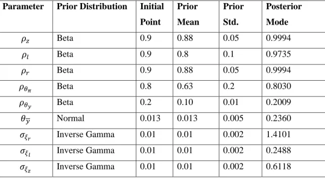
In order to make a comparison between the linear model and the nonlinear model we estimated the model with Kalman filter too. The estimated values can be found in Table 3.
Table 3 Kalman Filter Estimation Results Parameter Prior Distribution Initial
Point Prior Mean Prior Std. Posterior Mode 𝜌𝑧 Beta 0.9 0.88 0.05 0.9994 𝜌𝑙 Beta 0.9 0.8 0.1 0.9735 𝜌𝑟 Beta 0.9 0.88 0.05 0.9994 𝜌𝜃𝜋 Beta 0.8 0.63 0.2 0.8030 𝜌𝜃𝑦 Beta 0.2 0.10 0.01 0.2009 𝜃𝑦 Normal 0.013 0.013 0.005 0.2360 𝜎𝜉𝑟 Inverse Gamma 0.01 0.01 0.002 1.4101 𝜎𝜉𝑙 Inverse Gamma 0.01 0.01 0.002 0.2488 𝜎𝜉𝑧 Inverse Gamma 0.01 0.01 0.002 0.6118
20
As we can see that since there is no stochastic volatility of the monetary policy shock, monetary policy shock itself tries to account for the whole changes in the monetary policy therefore its variance is so big. Another crucial difference is that coefficient of interest rate smoothing is almost 1, and it actually says that monetary policy mainly does not depend on the changes in the inflation rate in Turkey, which is not sensible at all. Besides, the steady states level of the Taylor Rule parameter on output difference is 0.2360, which is almost twenty times higher than the one in particle filter side13.
13 Even when we use simple OLS regression for the monetary policy rule we find the estimated values of
the 𝜃𝜋 is around 0.02, which is much more close to particle filter result compared to the Kalman filter
21 CHAPTER 4
SOLUTİON AND THE DYNAMICS 4.1) Solution
In our models we have 18 state variables, 3 innovations to the structural shocks (𝜉𝑧,𝑡, 𝜉𝑙,𝑡, 𝜉𝑟,𝑡), 3 innovations to the volatility shocks (𝑈𝑧,𝑡, 𝑈𝑙,𝑡, 𝑈𝑟,𝑡), and 2
innovations to the parameter drifts (𝜉𝜋,𝑡, 𝜉𝑦,𝑡), hence as in FGR (2010) we will use the perturbation method14. Since most of the literature linearize or log-linearize the model
around the steady state, they use the first order perturbation method. However, in our model we add the time varying volatilities and in order to capture this second order information we haven’t linearize the model otherwise it will be certainty equivalence. Besides, we need to solve the model with at least second order perturbation method, otherwise time varying volatilities disappear and don’t have an impact on the economy. As stated in Andreasen et al. (2016) even though first order approximations are stable, second order approximation can be unstable because of the explosive sample path15.
However, Kim, Kim, Schaumburg and Sims (2008) proposes a solution to get rid of this explosive sample path, called pruning meaning that do not include the terms that have
14As an alternative we have could use the value function iteration, but then we have to take 26 variables
into consideration, and it almost makes impossible to use this kind of solution method.
15 For illustrative example for explanation of how higher order approximations can be unstable you can
22
higher order effects than the order of the approximation16. In our case, we will solve the
model with second order approximation so the system of solution should not include the third and higher effects. Similar to example given in Andreasen et al. (2016), we will have a solution for Zt and since we have second order approximation it will be a function
of 𝑍𝑡−1𝑍𝑡−2, 𝑍𝑡−12 , 𝑍𝑡−22 . In the same method Zt-1 will be a function of 𝑍𝑡−22 . If we put
quadratic function of 𝑍𝑡−22 instead of Zt-1, then Zt will be a function of 𝑍𝑡−2 , 𝑍𝑡−22 , 𝑍𝑡−23 ,
𝑍𝑡−24 . Pruning will leave out the terms 𝑍𝑡−23 , 𝑍𝑡−24 since they are the third and fourth order effects, respectively. By using this methodology we solve the model with second order approximation.
4.2) Dynamics
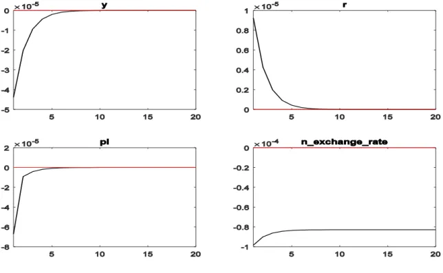
Since our non-linear DSGE model is hugely complicated we cannot obtain the closed form solution. Instead we are interested in the simulation results in a consequence of shocks hit the economy. In Figure 2, we have a one standard deviation shock17 to the monetary policy, then nominal interest will go up and the effect completely dies up after 2 years18.
It also affects the level of prices and the output negatively.
16 Even though we lose information when we exclude those terms, Andreasen et al. (2016) compares the
root mean squared Euler-equation errors (RMSE) of the first, second and third order pruned system and not pruned system. It shows that average error of the system with pruning is less than the average error of the system without pruning, hence losing that much information is not a big issue in that case.
17 The magnitude of all shocks are positive one standard deviation, and the simulation results are
obtained from Dynare.
23
Figure 2 The Impulse Response Functions to a Monetary Policy Shock (PF)19
In Figure 3, we have a one standard deviation shock to the monetary policy volatility shock, even if the results are not smooth as in Figure 1, initial reaction quite similar to each other. When we have a volatility shock that hit the economy, actually we change the volatility of the gross interest rate, and hence we change the uncertainty of gross interest rate. Then agents will save more. Compared to the Figure 2, inflation rate does not decrease initially in this case.
19 PF and KF stand for the results under the Particle Filter estimation and the Kalman Filter estimation,
24
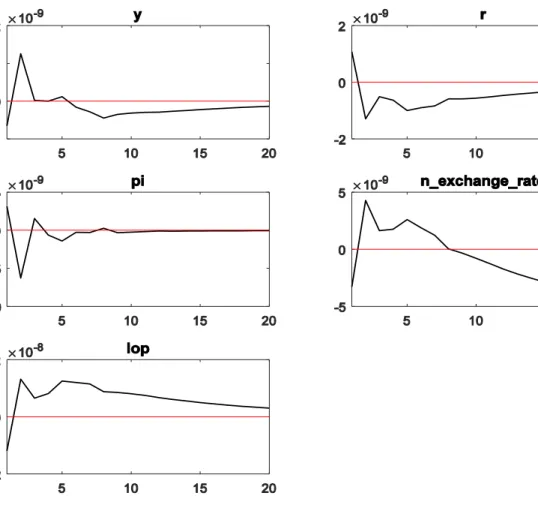
Figure 3 The Impulse Response Functions to a Monetary Policy Volatility Shock (PF)
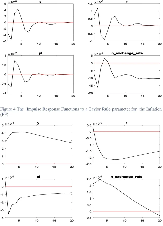
In Figure 4 and Figure 5, we have a shock to Taylor Rule parameter for the inflation and Taylor Rule parameter for the change in the output levels, respectively.
25
Figure 4 The Impulse Response Functions to a Taylor Rule parameter for the Inflation (PF)
Figure 5 The Impulse Response Functions to a Taylor Rule parameter for the Change in the Output Level (PF)
26
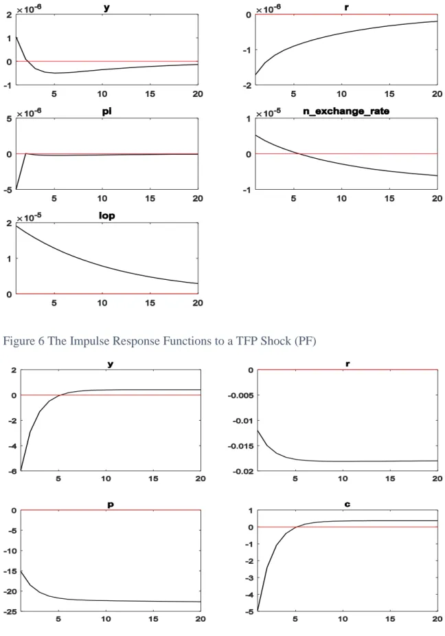
Figure 6 The Impulse Response Functions to a TFP Shock (PF)
27
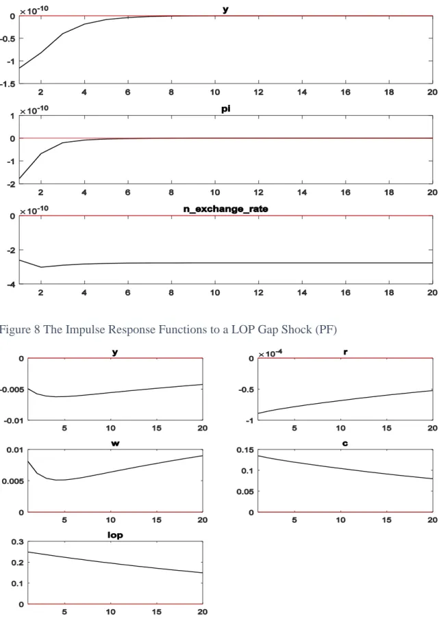
Figure 8 The Impulse Response Functions to a LOP Gap Shock (PF)
28
4.3) Evolution of the Taylor Rule parameter for Inflation
As we can see in the Table 1, the response of the monetary policy to the change in output level is quite small, hence it is more interesting to consider the evolution of the Taylor Rule parameter on inflation, this is actually more intuitive and more reasonable because as we stated earlier the main objective of the Central Bank of Turkey (CBT) is to achieve and maintain the price stability in Turkey, so evolution of this parameter actually is a clue about the thought of CBT on inflation. We can also see the response of CBT on inflation throughout the history hence we can comment on it whether they had really good policy or not. In the following two figures show the inflation rate in Turkey and smoothed path for the Taylor Rule on inflation, respectively. The orange shaded area shows pre-implicit inflation targeting period, the gray shaded region shows implicit inflation targeting period, and the rest of the region shows the post implicit inflation targeting period or explicit inflation targeting period. As we can notice that, from 1998Q1 to 2002Q1 this parameter starts from around 0 level and reached above 1 in this period. At the same time we observe that inflation rate falls from around 100% to 40% until 2001Q1. Even though this parameter sharply goes up in year 2001, inflation rate reacts in opposite way. The reason comes from the history of Turkey since Turkey has faced 2001 Turkish economic crisis during this period. Importantly, even though the same parameter in FGR (2010) is not affected by two oil shocks in U.S., in our case we can see the negative effects of this crisis on the estimated 𝜃𝜋,𝑡 . Moreover, although this parameter does not change too much during the implicit inflation targeting period and around 1.3 on average, inflation rate falls from around 60% to 10%. Even though they react to inflation in the same way, it decreases tremendously. So we expect that good luck instead of good policy mostly works during
29 Figure 10 Inflation Rate in Turkey (%)
30
this period. For the rest of the area we have seen that mostly this parameter is around 2 and the inflation rate is around 10% or in single digit. But still in these periods good luck should take place for example for the periods 2009 and 2010 although the parameter decreases, inflation rate declines as well.
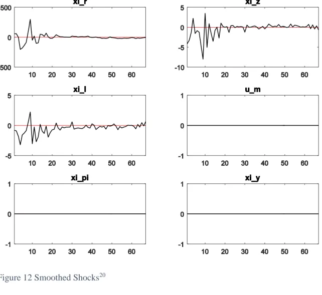
Figure 12 Smoothed Shocks20
20 In this figure, xi_r, xi_z, xi_l, u_m, xi_pi, xi_y represent the ξ
r, ξz,ξl, Ur,ξπ,ξy, respectively. X axis
shows the values from 0 to 71, where 0 corresponds 1998Q1 and 71 corresponds 2014Q3. Y axis shows the estimate of the smoothed structural shocks (deviations from their steady state levels). Notice that Ur,𝜉π,𝜉y do not evolve over time because they do not have a stochastic volatility.
31
Figure 12 proves the good luck argument after the period 2002, we see that there is a substantial decline in the stochastic volatility after that period in Turkish economy. Since SV decreases, uncertainty decreases as well. Combining with the fact that the Taylor Rule parameter on Inflation increases on average during this period, we concluded that our estimated model suggest that both good policy and good luck played roles in bringing down the inflation.
32
CHAPTER 4
CONCLUSION
In this paper we try to account for the decline in inflation in Turkey. To do better off we follow both Monacelli (2005) and FGR (2010) closely, and we build a nonlinear estimated DSGE model with law of one price gap, stochastic volatility and parameter drifting. Our main finding is that the success in decline in inflation after 2002 is not just because of the good policy, it is actually combination of both good policy and good luck.
This thesis can be extended in the future in the following ways; first because of the time constraint we could not estimate all parameters in the model all parameters can also be estimated. Second, we assume that there is a complete financial market to make our small open economy model stationary, by assuming one of the other 4 ways to make such a model stationary in Schmitt-Grohe and Uribe (2003) we can relax the complete financial market assumption. Third, for the small open economies like Turkey, exchange rate is a crucial part of the monetary policy hence we can add it into the policy rule so that we can see the effects of the incomplete pass-through of exchange rate over the policy rule more clearly. Fourth, we use the second order perturbation method to solve the model, we can extend it to the third order perturbation method because it will allow us the independent effects of volatility shocks. The reason why we should stop at the third order solution is
33
that Aruoba S. B. et al. (2006) compares the perturbation method to global solution methods such as value function iteration and collocation. When they solve the model up to fifth order, they see that beyond the third order the accuracy of the perturbation method does not increase so much hence third order perturbation solution is pretty good.
Moreover, we can use forecast error variance decomposition (FEVD) and historical decomposition (HD). By using former one we can find the average contribution of the structural shocks to the variance of the series. By using latter, we can see the actual contribution of the structural shocks to the level of the time series.
34
BIBLIOGRAPHY
Andreasen, M. M., Fernandez-Villaverde, J., and Rubio-Ramirez, J. F. (2016), “The Pruned State-Space Systems for Non-Linear DSGE Models: Theory and Empirical
Applications”, NBER Working Paper.
Calvo, G.A. (1983), “Staggered Prices in a Utility-maximizing Framework,” Journal of Monetary Economics, Elsevier, vol. 12(3), pages 383-398, September.
Denhaan, W. J., and Wind J. (2012), "Nonlinear and stable perturbation-based approximations." Journal of Economic Dynamics and Control 36.10: 1477-1497.
Hall, R.E. (1978). “Stochastic Implications of the Life Cycle-Permanent Income Hypothesis: Theory and Evidence”, Journal of Political Economy, University of Chicago Press, vol. 86(6), pages 971-87, December.
Kara, A. H., and Orak, M. (2008) “Enflasyon Hedeflemesi” Central Bank of the Republic of Turkey Conference Paper, October.
Kim, J., Kim, S., Schaumburg, E., and Sims, C. A. (2008), “Calculating and using second order accurate solutions of discrete time dynamic equilibrium models”, Journal of Economic Dynamics and Control, 32(11), 3397-3414.
35
Monacelli, T (2005), “Monetary policy in a low pass-through environment”, Journal of Money Credit and Banking, 37(6), 1047–1066.
Aruoba, S. B. Fernandez-Villaverde, J., Rubio-Ramirez, J. F. (2006), “Comparing solution methods for dynamic equilibrium economies”, Journal of Economic Dynamics & Control, pages 2477-2508.
Schmitt-Grohe, S. & Uribe, M. (2003), “Closing small open economy models”, Journal of International Economics, Elsevier, vol. 61(1), pages 163-185, October.
Sims, E. (2014) “Graduate Macro Theory II,”
(http://www3.nd.edu/~esims1/grad_macro_14.html).
Villaverde-Fernandez, J., Guerrón-Quintana, P., and Rubio-Ramírez, J. F. (2010), “Reading the Recent Monetary History of the United States, 1959-2007”, Federal Reserve Bank of St. Louis Review.
Villaverde-Fernandez, J., Rubio-Ramírez, J. F., (2004), “Sequential Monte Carlo Filtering: an Example”.