High volatility, thick tails and extreme value theory
in value-at-risk estimation
Ramazan Gençay
a,∗, Faruk Selçuk
b,1, Abdurrahman Ulugülyaˇgci
baDepartment of Economics, Carleton University, 1125 Colonel By Drive, Ottawa, Ont., Canada K1S 5B6 bDepartment of Economics, Bilkent University, Bilkent 06533, Ankara, Turkey
Received 1 August 2002; received in revised form 3 May 2003; accepted 29 July 2003
Abstract
In this paper, the performance of the extreme value theory in value-at-risk calculations is compared to the performances of other well-known modeling techniques, such as GARCH, variance–covariance (Var–Cov) method and historical simulation in a volatile stock market. The models studied can be classified into two groups. The first group consists of GARCH(1, 1) and GARCH(1, 1)-t models which yield highly volatile quantile forecasts. The other group, consisting of historical simula-tion, Var–Cov approach, adaptive generalized Pareto distribution (GPD) and nonadaptive GPD models, leads to more stable quantile forecasts. The quantile forecasts of GARCH(1, 1) models are excessively volatile relative to the GPD quantile fore-casts. This makes the GPD model be a robust quantile forecasting tool which is practical to implement and regulate for VaR measurements.
© 2003 Elsevier B.V. All rights reserved. JEL classification: G0; G1; C1
Keywords: Value-at-risk; Financial risk management; Extreme value theory
1. Introduction
The common lesson from financial disasters is that billions of dollars can be lost because of poor supervision and management of financial risks. The value-at-risk (VaR) was developed in response to financial disasters of the 1990s and obtained an in-creasingly important role in market risk management. The VaR summarizes the worst loss over a target horizon with a given level of confidence. It is a pop-ular approach because it provides a single quantity
∗Corresponding author. Fax:+1-208-693-7012.
E-mail addresses: [email protected] (R. Gençay), [email protected] (F. Selçuk).
1Tel.:+90-312-290-2074; fax: +90-208-694-3196.
that summarizes the overall market risk faced by an institution or an individual investor.2
In a VaR context, precise prediction of the probabil-ity of an extreme movement in the value of a portfolio is essential for both risk management and regulatory purposes. By their very nature, extreme movements are related to the tails of the distribution of the underly-ing data generatunderly-ing process. Several tail studies, after the pioneering work byMandelbrot (1963a,b), indicate that most financial time series are fat-tailed.3Although
2 See Dowd (1998),Jorion (1997)and Duffie and Pan (1997) for more details on the VaR methodology. For the regulatory roots of the VaR, seeBasel (1996).
3 See, for example,Dacorogna et al. (2001a,b),Hauksson et al.
(2001), Müller et al. (1998), Pictet et al. (1998), Danielsson and de Vries (1997), Ghose and Kroner (1995), Loretan and Phillips (1994), Hols and de Vries (1991), Koedijk et al.
0167-6687/$ – see front matter © 2003 Elsevier B.V. All rights reserved. doi:10.1016/j.insmatheco.2003.07.004
338 R. Gençay et al. / Insurance: Mathematics and Economics 33 (2003) 337–356
these findings necessitate a definition of what is meant by a fat-tailed distribution, there is no unique definition of fat-tailness (heavy-tailness) of a distribution in the literature.4In this study, we consider a distribution to be fat-tailed if a power decay of the density function is observed in the tails. Accordingly, an exponential de-cay or a finite endpoint at the tail (the density reaching zero before a finite quantile) is treated as thin-tailed.5 In order to model fat-tailed distributions, the log-normal distribution, generalized error distribution, and mixtures of normal distributions are suggested in many studies. However, these distributions are thin-tailed according to our definition since the tails of these distributions decay exponentially, although they have excess kurtosis over the normal distribution. In some practical applications, these distributions may fit the empirical distributions up to moderate quan-tiles but their fit deteriorates rapidly at high quanquan-tiles (at extremes).
An important issue in modeling the tails is the finiteness of the variance of the underlying distribu-tion. The finiteness of the variance is related to the thickness of the tails and the evidence of heavy tails in financial asset returns is plentiful. In his seminal work,Mandelbrot (1963a,b)advanced the hypothesis of a stable distribution on the basis of an observed invariance of the return distribution across different frequencies and apparent heavy tails in return distri-butions. The issue is that while the normal distribu-tion provides a good approximadistribu-tion to the center of the return distribution for monthly (and lower) data frequencies, there is strong deviation from normality for frequencies higher than monthly frequency. This implies that there is a higher probability of extreme values than for a normal distribution.6 Mandelbrot (1963a,b)provided empirical evidence that the stable Levy distributions are natural candidates for return
(1990),Boothe and Glassman (1987),Levich (1985)andMussa (1979).
4 SeeEmbrechts et al. (1997, Chapters 2 and 8)for a detailed discussion.
5 Although the fourth moment of an empirical distribution (sam-ple kurtosis) is sometimes used to decide on whether an empirical distribution is heavy-tailed or not, this measure might be mis-leading. For example, the uniform distribution has excess kurtosis over the normal distribution but it is thin-tailed according to our definition.
6 This indicates that the fourth moment of the return distribution is larger than expected from a normal distribution.
distributions. For excessively fat-tailed random vari-ables whose second moment does not exist, the stan-dard central limit theorem no longer applies, however, the sum of such variables converge to Levy distri-bution within a generalized central limit theorem. Later studies,7however, demonstrated that the return behavior is much more complicated, and follows a power law, which is not compatible with the Levy distribution.
Instead of forcing a single distribution for the entire sample, it is possible to investigate only the tails of the sample distribution using limit laws, if only the tails are important for practical purposes. Furthermore, the parametric modeling of the tails is convenient for the extrapolation of probability assignments to the quan-tiles even higher than the most extreme observation in the sample. One such approach is the extreme value theory (EVT) which provides a formal framework to study the tail behavior of the fat-tailed distributions.
The EVT stemming from statistics has found many applications in structural engineering, oceanography, hydrology, pollution studies, meteorology, material strength, highway traffic and many others.8 The link between the EVT and risk management is that EVT methods fit extreme quantiles better than the conven-tional approaches for heavy-tailed data.9 The EVT approach is also a convenient framework for the sep-arate treatment of the tails of a distribution which allows for asymmetry. Considering the fact that most financial return series are asymmetric (Levich, 1985; Mussa, 1979), the EVT approach is advantageous over models which assume symmetric distributions such as t-distributions, normal distributions, ARCH, GARCH-like distributions except E-GARCH which allows for asymmetry (Nelson, 1991). Our findings indicate that the performance of conditional risk management strategies, such as ARCH and GARCH, is relatively poor as compared to unconditional ap-proaches.
The paper is organized as follows. The EVT and VaR estimation are introduced in Sections 2 and 3.
7SeeKoedijk et al. (1990),Mantegna and Stanley (1995),Lux
(1996),Müller et al. (1998)andPictet et al. (1998).
8For an in-depth coverage of EVT and its applications in finance and insurance, seeEmbrechts et al. (1997),McNeil (1998),Reiss and Thomas (1997)andTeugels and Vynckier (1996).
9See Embrechts et al. (1999) and Embrechts (2000a)for the efficiency of EVT as a risk management tool.
Empirical results from a volatile market are presented inSection 4. We conclude afterwards.
2. Extreme value theory
From the practitioners’ point of view, one of the most interesting questions that tail studies can answer is what are the extreme movements that can be ex-pected in financial markets? Have we already seen the largest ones or are we going to experience even larger movements? Are there theoretical processes that can model the type of fat tails that come out of our empir-ical analysis? Answers to such questions are essential for sound risk management of financial exposures. It turns out that we can answer these questions within the framework of the EVT. Once we know the tail index, we can extend the analysis outside the sample to con-sider possible extreme movements that have not yet been observed historically. This can be achieved by computation of the quantiles with exceedance proba-bilities.
EVT is a powerful and yet fairly robust frame-work to study the tail behavior of a distribution. Even though EVT has previously found large applicability in climatology and hydrology, there have also been a number of extreme value studies in the finance liter-ature in recent years.de Haan et al. (1994)study the quantile estimation using the EVT.Reiss and Thomas (1997) is an early comprehensive collection of sta-tistical analysis of extreme values with applications to insurance and finance, among other fields.McNeil (1997, 1998) studies the estimation of the tails of loss severity distributions and the estimation of the quantile risk measures for financial time series using EVT.Embrechts et al. (1999)overview the EVT as a risk management tool.Müller et al. (1998)andPictet et al. (1998) study the probability of exceedances for the foreign exchange rates and compare them
with the GARCH and HARCH models. Embrechts
(1999, 2000a) studies the potentials and limitations of the EVT. McNeil (1999) provides an extensive overview of the EVT for risk managers. McNeil and Frey (2000) study the estimation of tail-related risk measures for heteroskedastic financial time se-ries. Embrechts et al. (1997), Embrechts (2000b) and Reiss and Thomas (1997) are comprehensive sources of the EVT to the finance and insurance literature.
3. Value-at-risk
Letrt = log(pt/pt−1) be the returns at time t where
pt is the price of an asset (or portfolio) at time t. The VaRt(α) at the (1 − α) percentile is defined by Pr(rt ≤ VaRt(α)) = α, (1) which calculates the probability that returns at time
t will be less than (or equal to) VaRt(α), α percent of the time.10 The VaR is the maximum potential increase in value of a portfolio given the specifica-tions of normal market condispecifica-tions, time horizon and a level of statistical confidence. The VaR’s popular-ity originates from the aggregation of several compo-nents of risk at firm and market levels into a single number.
The acceptance and usage of VaR has been spread-ing rapidly since its inception in the early 1990s. The VaR is supported by the group of 10 banks, the group of 30, the Bank for International Settlements, and the European Union. The limitations of the VaR are that it may lead to a wide variety of results under a wide variety of assumptions and methods; focuses on a sin-gle somewhat arbitrary point; explicitly does not ad-dress exposure in extreme market conditions and it is a statistical measure, not a managerial/economic one.11
The methods used for VaR can be grouped under the parametric and nonparametric approaches. In this paper, we study the VaR estimation with EVT which is a parametric approach. The advantage of the EVT is that it focuses on the tails of the sample distribu-tion when only the tails are important for practical purposes. Since fitting a single distribution to the en-tire sample imposes too much structure and our need here is the tails, we adopt the EVT framework which is what is needed to calculate the VaR. We compare the VaR calculations with EVT and its performance to the variance–covariance (Var–Cov) method (para-metric, unconditional volatility), historical simulation (nonparametric, unconditional volatility), GARCH
10A typical value ofα is 5 or 1%.
11There is a growing consensus among both academicians and practitioners that the VaR as a measure of risk has serious defi-ciencies. See the special issue of Journal of Banking and Finance 26 (7) (2002) on “Statistical and Computational Problems in Risk Management: VaR and Beyond VaR”.
340 R. Gençay et al. / Insurance: Mathematics and Economics 33 (2003) 337–356
(1, 1)-t and GARCH(1, 1) with normally distributed innovations (parametric, conditional volatility).
The Var–Cov method is the simplest approach among the various models used to estimate the VaR. Let the sample of observations be denoted by rt, t = 1, 2, . . . , n, where n is the sample size. Let us assume that rt follows a martingale process with rt = µt + t, where has a distribution function F with zero mean and variance, σt2. The VaR in this case can be calculated as
VaRt(α) = ˆµt+ F−1(α)ˆσt, (2)
where F−1(α) is the qth quantile (q = 1 − α) value of the unknown distribution function F. An esti-mate ofµt andσt2 can be obtained from the sample mean and the sample variance. Although sample variance as an estimator of the standard deviation in Var–Cov approach is simple, it has drawbacks at high quantiles of a fat-tailed empirical distribution. The quantile estimates of the Var–Cov method for the right tail (left tail) are biased downwards (up-wards) for high quantiles of a fat-tailed empirical distribution. Therefore, the risk is underestimated with this approach. Another drawback of this method is that it is not appropriate for asymmetric distri-butions. Despite these drawbacks, this approach is commonly used for calculating the VaR from holding a certain portfolio, since the VaR is additive when it is based on sample variance under the normality assumption.
Instead of the sample variance, the standard devia-tion inEq. (2)can be estimated by a statistical model. Since financial time series exhibit volatility cluster-ing, the autoregressive conditional heteroscedasticity (ARCH) (Engle, 1982) and the generalized autore-gressive conditional heteroscedasticity (GARCH) (Bollerslev, 1982) are popular models in practice. Among other studies, Danielsson and Moritomo (2000)andDanielsson and de Vries (2000)show that these conditional volatility models with frequent pa-rameter updates produce volatile estimates, and are not well suited for analyzing large risks. Our findings provide further evidence that the performance of con-ditional risk management strategies, such as ARCH and GARCH, is relatively poor as compared to un-conditional approaches. The performance of these conditional models worsens as one moves further in the tail of the losses.
4. Empirical findings
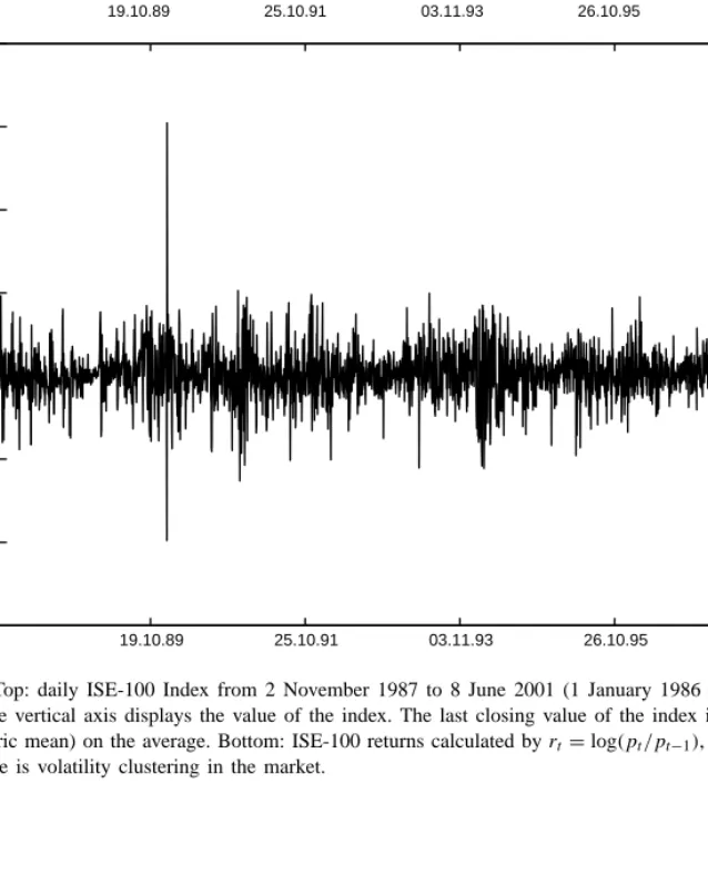
A volatile market provides a suitable environment to study the relative performance of competing VaR modeling approaches. In this regard, the Turkish econ-omy is a good candidate.12 The Istanbul Stock Ex-change was formally inaugurated at the end of 1985. Following the capital account liberalization in 1989, foreign investors were allowed to purchase and sell all types of securities and repatriate the proceeds. The to-tal market value of all traded companies was only US$ 938 million in 1986 and reached a record level of US$ 114.3 billion in 1999. Following a major financial cri-sis in February 2001, the total market value of all listed companies went down to 33.1 billion by November 2001. The daily average trade volume also decreased from the record level US$ 740 million in 2000 to US$ 336 million in November 2001.Figs. 1 and 2clearly indicate the high volatility and thick-tail nature of the Istanbul Stock Exchange Index (ISE-100), making it a natural platform to study EVT in financial markets.
4.1. Data analysis
The data set is the daily closings of the Istanbul Stock Exchange (ISE-100) Index from 2 November 1987 to 8 June 2001. The index value is normalized to 1 at 1 January 1986 and there are 3383 observa-tions in the data set. The daily returns are defined by rt = log(pt/pt−1), where pt denotes the value of the index at day t. In the top panel ofFig. 1the level of the ISE-100 Index is presented. The corresponding daily returns are displayed in the bottom panel ofFig. 1. The average daily return is 0.22% which implies ap-proximately 77% annual return (260 business days).13 This is not surprising as the economy is a high infla-tion economy. However, 3.27% daily standard devia-tion indicates a highly volatile environment. Indeed, extremely high daily returns (as high as 30.5%) or daily losses (as low as−20%) are observed during the sample period. Also from a foreign investor’s point of view, ISE-100 exhibits a wide degree of fluctuations which is reflected in its US dollar value. In US dollar
12For an overview of the Turkish economy in recent years, see
Ertuˇgrul and Selçuk (2001). Gençay and Selçuk (2001) study the recent crises episode in the Turkish economy from the risk management point of view.
19.10.89 25.10.91 03.11.93 26.10.95 28.10.97 17.11.99 0 0.4 0.8 1.2 1.6 2 x 10 4 19.10.89 25.10.91 03.11.93 26.10.95 28.10.97 17.11.99 –0.2 –0.1 0 0.1 0.2 0.3 0.4
Fig. 1. Top: daily ISE-100 Index from 2 November 1987 to 8 June 2001 (1 January 1986= 1). The horizontal axis corresponds to time while the vertical axis displays the value of the index. The last closing value of the index is 12138.26, implying a daily return of 0.22% (geometric mean) on the average. Bottom: ISE-100 returns calculated byrt= log(pt/pt−1), where ptis the value of the index at t. Notice that there is volatility clustering in the market.
342 R. Gençay et al. / Insurance: Mathematics and Economics 33 (2003) 337–356 –0.40 –0.3 –0.2 –0.1 0 0.1 0.2 0.3 50 1 00 1 50 2 00 2 50 3 00 0.1 0.15 0.2 0.25 0.3 0 5 10 15 20 25
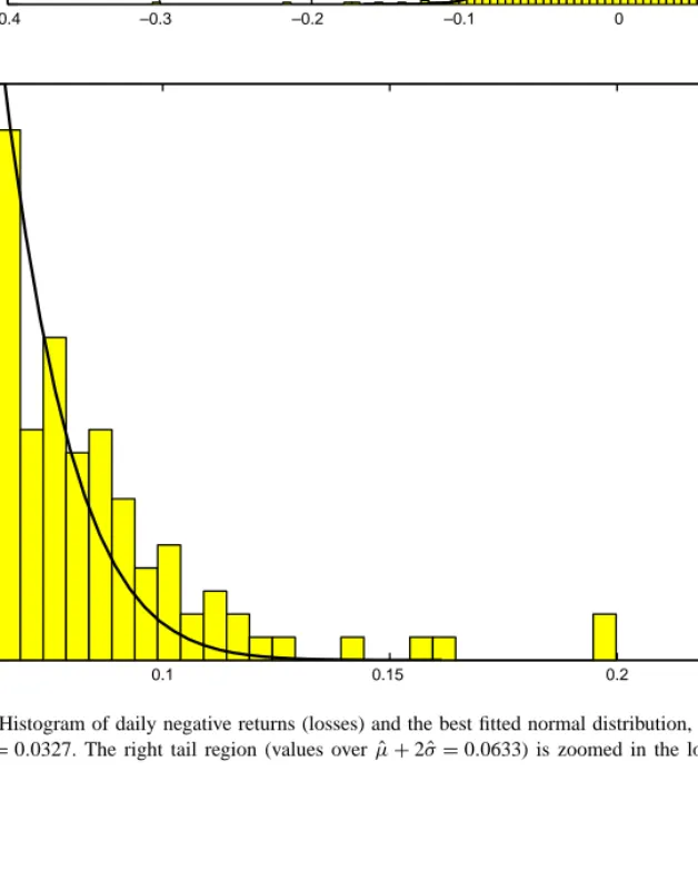
Fig. 2. Histogram of daily negative returns (losses) and the best fitted normal distribution,N( ˆµ, ˆσ). Estimated parameters are ˆµ = −0.0022 and ˆσ = 0.0327. The right tail region (values over ˆµ + 2 ˆσ = 0.0633) is zoomed in the lower panel which indicates a heavy tail.
terms (1986 = 100), the ISE-100 reached a record level of 1654 at the end of the year 1999 and dropped down to 378 in November 2001.
The sample skewness and kurtosis are 0.18 and 8.21, respectively. Although there is no significant skewness, there is excess kurtosis. In the framework of this paper, the fat-tailness may not be based on a normality test. Normality tests, such as theBera and Jarque (1981)normality test, based on sample skew-ness and sample kurtosis, may not be appropriate since rejecting normality due to a significant skewness or a significant excess kurtosis does not necessarily imply fat-tailness. For instance, a distribution may be skewed and thin-tailed or the empirical distribution may have excess kurtosis over normal distribution with thin-tails. The first 300 autocorrelations and partial autocorrela-tions of squared returns are statistically significant at several lags. This indicates volatility clustering and a GARCH type modeling should be considered in VaR estimations.
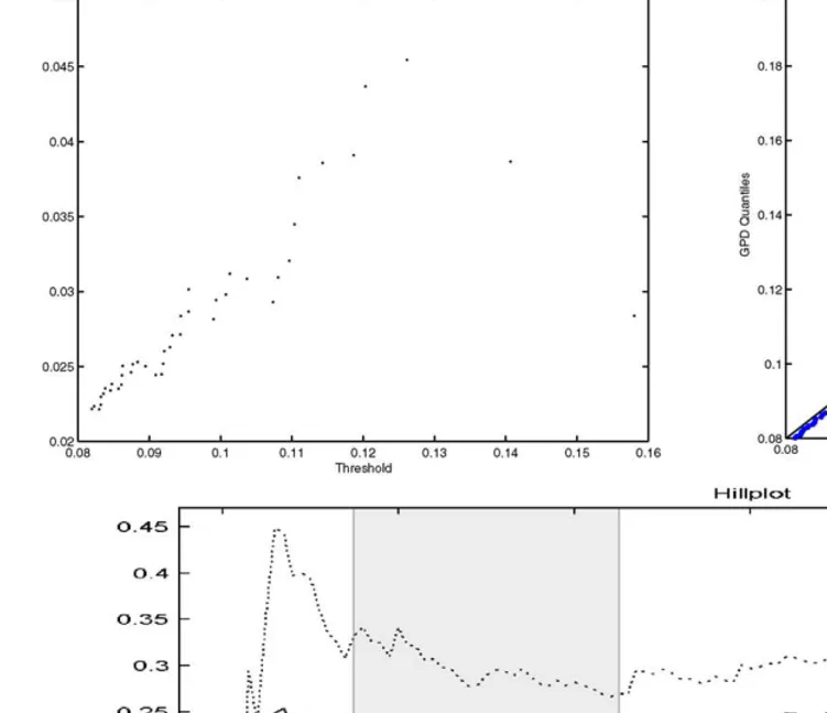
Other important tools for the examination of fat-tailness in the data are the sample histogram, QQ (quantile–quantile) plot and the mean excess function.14 The sample histogram of negative returns (returns multiplied with −1) is presented in Fig. 2. Extreme value analysis works with the right tail of the distribution. Hence, we work with negative re-turn distribution where the right tail corresponds to losses.15Fig. 2indicates that extreme realizations are more likely than a normal distribution would imply. The mean excess plot in the top-left panel ofFig. 3 in-dicates a heavy right tail for the loss distribution. QQ plot gives some idea about the underlying distribution of a sample. Specifically, the quantiles of an empirical distribution are plotted against the quantiles of a hy-pothesized distribution. If the sample comes from the hypothesized distribution or a linear transformation of the hypothesized distribution, the QQ plot should be linear. In extreme value analysis and generalized Pareto models, the unknown shape parameter of the distribution can be replaced by an estimate as sug-gested by Reiss and Thomas (1997, p. 66). If there is a strong deviation from a straight line, then either the assumed shape parameter is wrong or the model
14See Reiss and Thomas (1997, Chapters 1 and 2) for some empirical tools for representing data and to check the validity of the parametric modeling.
15Hereafter, we will refer to negative returns as losses.
selection is not accurate. In our case, the QQ plot of losses in the top-right panel ofFig. 3provides further evidence for fat-tailness. The losses over a threshold are plotted with respect to generalized Pareto dis-tribution (GPD) with an assumed shape parameter 0.20. The plot clearly shows that the left tail of the distributions over the threshold value 0.08 is well approximated by GPD.
The Hill plot is used to calculate the shape param-eter ξ = 1/α, where α is the tail index. The shape parameterξ is informative regarding the limiting dis-tribution of maxima. If ξ = 0, ξ > 0 or ξ < 0, this indicates an exponentially decaying, power-decaying, or finite-tail distributions in the limit, respectively. The critical aspect of the Hill estimator is the choice of the number of upper order statistics. The Hill plot of losses is displayed in the bottom panel of Fig. 3. The stable portion of this figure implies a tail index estimate between 0.20 and 0.25. Therefore, the Hill estimator indicates a power-decaying tail with an ex-ponent which varies between 4 and 5. This means that if the probability of observing a return greater than r is p then the probability of observing a loss greater than kr is in between k−4p and k−5p.
4.2. Relative performance
We consider six different models for the one pe-riod ahead loss predictions at different tail quantiles. These models are Var–Cov approach, historical simu-lation, GARCH(1, 1), GARCH(1, 1)-t, adaptive GPD and nonadaptive GPD models.
For the first five models, we adopt a sliding win-dow approach with three different winwin-dow sizes for 500, 1000, and 2000 days.16 For instance, the win-dow is placed between first and 1000th observations for a window size of 1000 days and a given quantile is forecasted for the 1001st day. Next, the window is slided one step forward to forecast quantiles for 1002nd, 1003rd, . . . , 3382nd days. The motivation behind the sliding window technique is to capture dynamic time-varying characteristics of the data in different time periods. The last approach (nonadaptive GPD model) does not utilize a sliding window and uses all the available data up to the day on which fore-casts are generated. This approach is preferable since
16Danielsson and Moritomo (2000)also adopts a similar win-dowing approach.
344 R. Gençay et al. /Insur ance: Mathematics and Economics 33 (2003) 337–356
Fig. 3. Top-left: mean excess (ME) plot. The horizontal axis is for thresholds over which the sample mean of the excesses are calculated. Values on the vertical axis display the corresponding mean excesses. The positive trend for thresholds above approximately 0.082 indicates a heavy left tail since this is the mean excess plot for losses. Since an approximately linear positive trend in an ME plot results from a Pareto type behavior (tail probabilities decaying as a power function), the extreme losses in ISE-100 Index have
a Pareto type behavior. Top-right: QQ plot of losses with respect to a GPD (assumed shape parameter, ˆξ, is 0.20). It shows that the left tail of the distributions over the threshold
value 0.08 is well approximated by the GPD. Bottom: variation of the Hill estimate of the shape parameter across the number of upper order statistics. The Hill estimate is very sensitive to the number of upper order statistics. The estimator for the shape parameter should be chosen from a region where the estimate is relatively stable. A stable region is toned gray in the figure. Notice that the confidence bands decrease on the right side of this stability region since more upper order statistics are used to calculate the estimate.
GPD estimation requires more data for out-of-sample forecasts, as extreme events are rare.17
The GARCH models are parameterized as having one autoregressive and one moving average term, GARCH(1, 1), since it is practically impossible to find the best parameterization for each out-of-sample forecast of a given window size. A similar constraint also applies for the GPD modeling, i.e., the difficulty of choosing the appropriate threshold value for each run. Both the adaptive and nonadaptive GPD quantile forecasts are generated using the upper 2.5% of the sample. In principle, it is possible to choose different thresholds for different quantiles and different win-dow sizes but this would increase the effect of data snooping.18 For the historical simulation, piecewise linear interpolation is chosen to make the empirical distribution function one-to-one.19
The relative performance of each model is cal-culated in terms of the violation ratio. A violation occurs when a realized return is greater than the esti-mated return. The violation ratio is defined as the total number of violations, divided by the total number of one-period forecasts.20If the model is correct, the ex-pected violation ratio is the tail area for each quantile. At qth quantile, the model predictions are expected to be wrong (underpredict the realized return)α = (1−q) percent of the time. For instance, the model is expected to underpredict the realized return 5% of the time at the 95th quantile. A high violation ratio at each quantile implies that the model excessively underestimates the realized return (=risk). If the violation ratio at the qth quantile is greater than α percent, this implies
exces-17In extreme value analysis, we employed the EVIM toolbox of
Gençay et al. (2003).
18SeeSullivan et al. (2001)for the implications of data snooping in applied studies.
19There are other interpolation techniques such as nonlinear interpolation or nonparametric interpolation which can also be used.
20For example, for a sample size of 3000, a model with a window size of 500 days produces 2500 one-step-ahead return estimates for a given quantile. Each of these one-step-ahead returns is compared to the corresponding realized return. If the realized return is greater than the estimated return, a violation occurs. The ratio from total violations (total number of times a realized return is greater than the corresponding estimated return) to the total number of estimates is the violation ratio. If the number of violations is 125, the violation ratio at this particular quantile is 5%(125/2500 = 0.05). That is, 5% of the time the model underpredicts the return (realized return is greater than the estimated return).
sive underprediction of the realized return. If the viola-tion ratio is less thanα percent at the qth quantile, there is excessive overprediction of the realized return by the underlying model. For example, if the violation ratio is 2% at the 95th quantile, the realized return is only 2% of the time greater than what the model predicts.
It is tempting to conclude that a small violation ratio is always preferable at a given quantile. However, this may not be the case in this framework. Notice that the estimated return determines how much capital should be allocated for a given portfolio assuming that the investor has a short position in the market. Therefore, a violation ratio excessively greater than the expected ratio implies that the model signals less capital allo-cation and the portfolio risk is not properly hedged. In other words, the model increases the risk exposure by underpredicting it. On the other hand, a violation ratio excessively lower than the expected ratio implies that the model signals a capital allocation more than necessary. In this case, the portfolio holder allocates more to liquidity and registers an interest rate loss. A regulatory body may prefer a model overpredicting the risk since the institutions will allocate more capi-tal for regulatory purposes. Institutions would prefer a model underpredicting the risk, since they have to al-locate less capital for regulatory purposes, if they are using the model only to meet the regulatory require-ments. For this reason, the implemented capital allo-cation ratio is increased by the regulatory bodies for those models that consistently underpredict the risk.
Quantiles which are important for contemporary risk management applications as well as regula-tory capital requirements are 0.95th, 0.975th, 0.99th, 0.995th and 0.999th quantiles. Table 1 displays the violation ratios for the left tail (losses) at the window size of 1000 observations.21 The numbers in paren-theses are the ranking between six competing models for each quantile. Var–Cov method has the worst per-formance regardless of the window size except for the 95th quantile. Since quantiles higher than 0.95th are more of a concern in risk management applications, we can conclude that the Var–Cov method should be placed at the bottom of the performance ranking of competing models in this particular market. The
21To minimize the space for tables and the corresponding figures we report the results for the window size of 1000 observations. The findings for the window sizes of 500 and 2000 observations do not differ from the window size of 1000 observations significantly.
346 R. Gençay et al. / Insurance: Mathematics and Economics 33 (2003) 337–356 Table 1
VaR violation ratios for the left tail (losses) of daily ISE-100 returns (in %)a
5% 2.5% 1% 0.5% 0.1% Var–Cov 5.37 (2) 3.36 (5) 2.31 (6) 1.60 (5) 0.92 (6) Historical simulation 5.46 (3) 2.73 (2) 1.22 (3) 0.67 (1) 0.34 (4) GARCH(1, 1) 4.70 (1) 2.85 (4) 1.85 (5) 1.34 (4) 0.59 (5) GARCH(1, 1)-t 3.78 (6) 2.23 (3) 1.18 (2) 0.76 (3) 0.21 (2) Adaptive GPD 6.21 (5) 2.73 (2) 1.13 (1) 0.67 (1) 0.25 (3) Nonadaptive GPD 4.41 (4) 2.64 (1) 1.39 (4) 0.71 (2) 0.17 (1)
aThe numbers in parentheses are the ranking between six competing models for each quantile. The violation ratio of the best performing model is given in italics. Each model is estimated for a rolling window size of 1000 observations. The expected value of the VaR violation ratio is the corresponding tail size. For example, the expected VaR violation ratio at 5% tail is 5%. A calculated value greater than the expected value indicates an excessive underestimation of the risk while a value less than the expected value indicates an excessive overestimation. Daily returns are calculated from the ISE-100 Index. The sample period is 2 November 1987–8 June 2001. The sample size is 3383 observations. Data source: The Central Bank of the Republic of Turkey.
Table 2
VaR violation ratios for the right tail of daily ISE-100 returns (in %)a
5% 2.5% 1% 0.5% 0.1% Var–Cov 4.70 (2) 3.19 (5) 2.06 (6) 1.43 (6) 0.59 (6) Historical simulation 5.37 (3) 2.85 (4) 1.34 (3) 0.84 (4) 0.34 (4) GARCH(1, 1) 4.83 (1) 2.69 (2) 1.47 (5) 0.88 (5) 0.42 (5) GARCH(1, 1)-t 3.74 (6) 1.81 (5) 0.88 (1) 0.42 (1) 0.21 (2) Adaptive GPD 6.09 (4) 2.81 (3) 1.22 (2) 0.63 (2) 0.29 (3) Nonadaptive GPD 3.78 (5) 2.52 (1) 1.43 (4) 0.67 (3) 0.13 (1)
aThe numbers in parentheses are the ranking between six competing models for each quantile. Each model is estimated for a rolling window size of 1000 observations. The expected value of the VaR violation ratio is the corresponding tail size. For example, the expected VaR violation ratio at 5% tail is 5%. A calculated value greater than the expected value indicates an excessive underestimation of the risk while a value less than the expected value indicates an excessive overestimation. Daily returns are calculated from the ISE-100 Index. The sample period is 2 November 1987–8 June 2001. The sample size is 3383 observations. Data source: The Central Bank of the Republic of Turkey.
second worst model is GARCH(1, 1), except for its excellent performance at the 95th quantile. Although it performs better than the Var–Cov approach, even the simple historical simulation approach produces smaller VaR violation rates than the GARCH model for most quantiles.
At the 0.975th quantile, nonadaptive GPD per-forms the best with a violation ratio of 2.64% which amounts to 0.14% over-rejection. The adaptive GPD models follow with 2.73% (0.23% over-rejection) and GARCH-t ranks third with 2.23% (0.27% under-rejection). At the 0.99th quantile, the adaptive GPD provides the best violation ratio with 1.13% which is followed by GARCH-t with 1.18%. At the 0.995th quantile the adaptive GPD and historical sim-ulation provide the best violation ratios with 0.67% which is followed by adaptive GPD with 0.71%. At
the 0.999th quantile, nonadaptive GPD provides the best performance with 0.17% which is followed by GARCH-t with 0.21%. Overall, the results inTable 1 indicate that GPD models provide the best violation ratios for quantiles 0.975 and higher. GARCH-t comes close to being the third contender and competes with the historical simulation.
Table 2 displays the results for the right tail of returns.22 The Var–Cov method is again the worst model for the quantiles higher than the 0.95th quan-tile. GARCH(1, 1) performs best at the 0.95th and 0.975th quantiles but its performance deteriorates at higher quantiles. GARCH(1, 1)-t provides the best re-sults for quantiles higher than the 0.975th except the
22It is important to investigate both tails since a financial insti-tution may have a short position in the market.
0.999th quantile where nonadaptive GPD performs best. Adaptive GPD is the second best for 0.99th and 0.995th quantiles. Historical simulation is again an av-erage model.
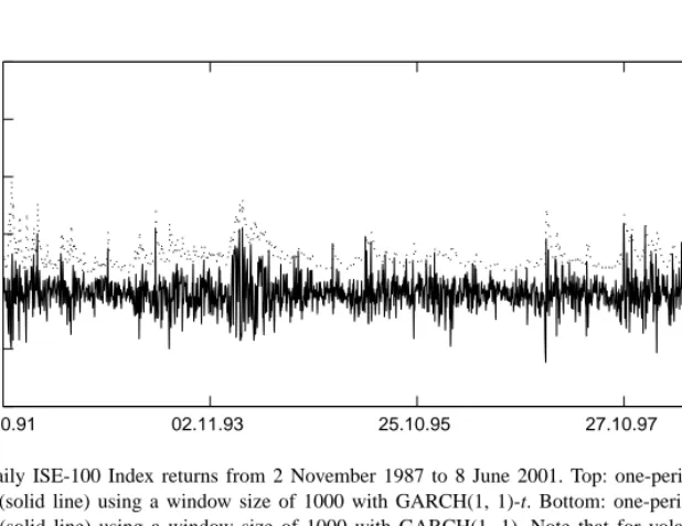
The one-period ahead 0.99th quantile forecasts of GARCH(1, 1) and GARCH(1, 1)-t models for losses are presented in Fig. 4 for the window size of 1000. Although the daily quantile forecasts of both models are quite volatile, GARCH(1, 1)-t model yields sig-nificantly higher, and therefore more volatile quantile forecasts relative to the GARCH(1, 1) model. This implies that the allocation of the capital for regu-latory purposes has to vary on a daily basis. This daily variation can be as large as 20% which is quite costly to implement and difficult to supervise in practice. 24.10.91 02.11.93 25.10.95 27.10.97 16.11.99 –0.2 –0.1 0 0.1 0.2 0.3 0.4 24.10.91 02.11.93 25.10.95 27.10.97 16.11.99 –0.2 –0.1 0 0.1 0.2 0.3 0.4
Fig. 4. Daily ISE-100 Index returns from 2 November 1987 to 8 June 2001. Top: one-period ahead 0.99th quantile forecasts (dotted line) of losses (solid line) using a window size of 1000 with GARCH(1, 1)-t. Bottom: one-period ahead 0.99th quantile forecasts (dotted line) of losses (solid line) using a window size of 1000 with GARCH(1, 1). Note that for volatile periods, GARCH(1, 1)-t gives significantly higher quantile estimates.
In the top panel of Fig. 5 quantile forecasts for the Var–Cov, historical simulation and adaptive GPD models are presented. All three models provide rather stable quantile forecasts across volatile return periods. The Var–Cov and historical simulation quantile casts are always lower than the adaptive GPD fore-casts with Var–Cov quantile forefore-casts being the most volatile between these three models.
A comparison between the GARCH(1, 1)-t and adaptive GPD model is presented in the bottom panel of Fig. 5. This comparison indicates that GARCH models yield very volatile quantile estimates when compared to the GPD, historical simulation or Var–Cov approaches. The volatility of the GARCH quantile forecasts are twice as much of the GPD quantile forecasts in a number of dates. Based on
348 R. Gençay et al. / Insurance: Mathematics and Economics 33 (2003) 337–356 24.10.91 02.11.93 25.10.95 27.10.97 16.11.99 –0.2 –0.15 –0.1 –0.05 0 0.05 0.1 0.15 0.2 Losses Var – Cov HS GPD 24.10.91 02.11.93 25.10.95 27.10.97 16.11.99 –0.2 –0.1 0 0.1 0.2 0.3 0.4 Losses GARCH – t GPD
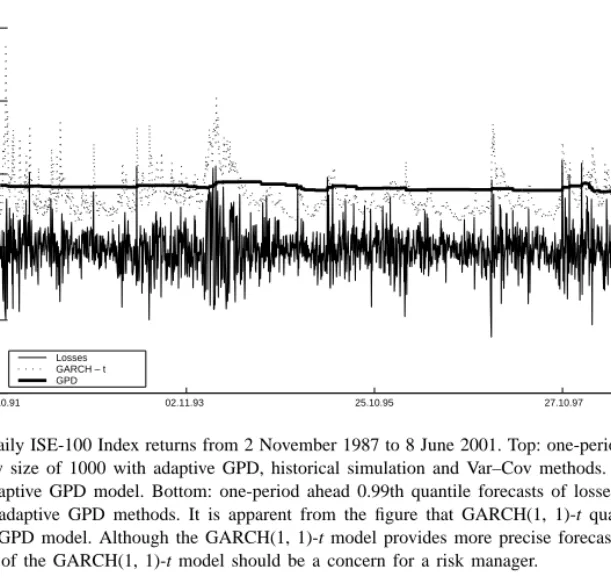
Fig. 5. Daily ISE-100 Index returns from 2 November 1987 to 8 June 2001. Top: one-period ahead 0.99th quantile forecasts of losses using a window size of 1000 with adaptive GPD, historical simulation and Var–Cov methods. The most conservative quantile forecasts belong to the adaptive GPD model. Bottom: one-period ahead 0.99th quantile forecasts of losses using a window size of 1000 with GARCH(1, 1)-t and adaptive GPD methods. It is apparent from the figure that GARCH(1, 1)-t quantile forecasts are much more volatile than the adaptive GPD model. Although the GARCH(1, 1)-t model provides more precise forecasts of this quantile, the excessive volatility of the forecasts of the GARCH(1, 1)-t model should be a concern for a risk manager.
Fig. 5, the level of change in the GARCH quantile forecasts can be as large 20–25% on a daily basis.
It is important that the models to be used in risk management should produce relatively stable quantile forecasts since adjusting the implemented capital fre-quently (daily) in light of the estimated VaR is costly
to implement and regulate. Therefore, models which yield more stable quantile forecasts may be more ap-propriate for the market risk management purposes. In this respect, the GPD models provide robust tail es-timates, and therefore more stable VaR projections in turbulent times.
4.3. S&P-500 returns
Although the Istanbul Stock Exchange Index returns provide an excellent environment to study the VaR models in high volatility markets with thick-tailed dis-tributions, this data set has not been studied widely in the literature and is not well known. Hence, we have repeated the same study with the S&P-500 Index re-turns.
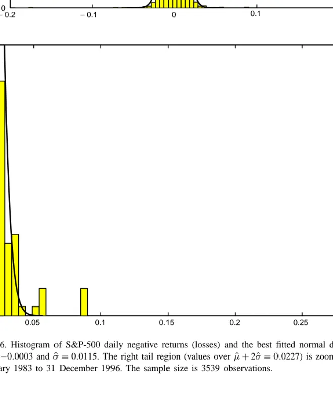
The data set is the daily closings of the S&P-500 Index from 3 January 1983 to 31 December 1996 and there are 3539 observations. The daily returns are de-fined byrt = log(pt/pt−1), where ptdenotes the value of the index at day t. The top panel of Fig. 6 pro-vides the histogram of the daily S&P-500 daily returns together with the best fitted normal distribution. The lower panel ofFig. 6provides the zoomed right tail which indicates thicker tails. The S&P-500 returns are highly skewed with a sample skewness of −6.5388 and has a large excess kurtosis with a sample kurtosis of 233.79.
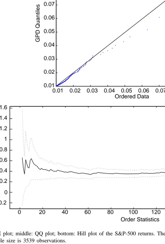
The mean excess plot in the top panel ofFig. 7 in-dicates a heavy right tail for the loss distribution. The QQ plot in the middle panel ofFig. 7provides further evidence for fat-tailness. The losses over a threshold are plotted with respect to the GPD with an assumed shape parameter, ˆξ = 0.30. It clearly shows that the left tail of the distributions over the threshold value 0.08 is well approximated by GPD. The Hill plot is used to calculate the shape parameterξ = 1/α, where α is the tail index. The shape parameter ξ is infor-mative regarding the limiting distribution of maxima. If ξ = 0, ξ > 0 or ξ < 0, this indicates an expo-nentially decaying, power-decaying, or finite-tail
dis-Table 3
VaR violation ratios for the left tail (losses) of daily S&P-500 returns (in %)a
5% 2.5% 1% 0.5% 0.1% Var–Cov 3.39 (4) 2.40 (1) 1.69 (5) 1.42 (5) 0.75 (5) Historical simulation 4.61 (3) 2.60 (1) 1.50 (4) 0.75 (3) 0.20 (2) GARCH(1, 1) 4.71 (2) 2.89 (3) 2.18 (6) 1.58 (6) 0.83 (4) GARCH(1, 1)-t 3.29 (6) 1.98 (4) 1.07 (1) 0.83 (4) 0.31 (3) Adaptive GPD 4.72 (1) 2.60 (1) 1.30 (3) 0.63 (2) 0.12 (1) Nonadaptive GPD 3.19 (5) 2.20 (2) 1.10 (2) 0.47 (1) 0.12 (1)
aThe numbers in parentheses are the ranking between six competing models for each quantile. Each model is estimated for a rolling window size of 1000 observations. The expected value of the VaR violation ratio is the corresponding tail size. For example, the expected VaR violation ratio at 5% tail is 5%. A calculated value greater than the expected value indicates an excessive underestimation of the risk while a value less than the expected value indicates an excessive overestimation. Daily returns are calculated from the S&P-500 Index. The sample period is 3 January 1983–31 December 1996. The sample size is 3539 observations. Data source: Datastream.
tributions in the limit, respectively. The Hill plot of losses is displayed in the bottom panel ofFig. 7. The stable portion of this figure implies a tail index esti-mate of 0.40. Therefore, the Hill estimator indicates a power-decaying tail with an exponent of 2.5.
Table 3displays the violation ratios for the left tail (losses) at the window size of 1000 observations. The numbers in parentheses are the ranking between six competing models for each quantile. Adaptive GPD model provides the best violation ratio for 0.95th and 0.975th quantiles. Var–Cov and historical simulation also do equally well with the adaptive GPD model for the 0.975th quantile. GARCH-t is the best performer for the 0.99th quantile which is followed by the adaptive GPD model. The nonadaptive GPD model provides the best performance for the 0.995th and 0.999th quantiles where the second best performer is the adaptive GPD model. The results from the left tail analysis indicate that GPD models provide the best vi-olation ratios in most quantiles. The ranking amongst the remaining three models is not obvious although Var–Cov method receives the worst violation ratios at the 0.99th quantiles and higher.Table 4displays the results for the right tail of returns. Amongst five quan-tiles, the adaptive GPD model performs as the best model by ranking first in three quantiles and the sec-ond in the remaining two quantiles. GARCH-t model has the worst performance in this tail by ranking as the last model except at the 0.999th quantile.
The S&P-500 one-period ahead 0.99th quantile forecasts of GARCH(1, 1) and GARCH(1, 1)-t mod-els for negative returns (losses) are presented inFig. 8 for the window size of 1000. Although the daily quantile forecasts of both models are quite volatile,
350 R. Gençay et al. / Insurance: Mathematics and Economics 33 (2003) 337–356 – 0.20 – 0.1 0 0.1 0.2 0.3 0.4 200 400 600 800 1000 1200 0.05 0.1 0.15 0.2 0.25 0.3 0.35 0.4 0 5 10 15 20 25 30
Fig. 6. Histogram of S&P-500 daily negative returns (losses) and the best fitted normal distribution,N( ˆµ, ˆσ). Estimated parameters are ˆµ = −0.0003 and ˆσ = 0.0115. The right tail region (values over ˆµ + 2 ˆσ = 0.0227) is zoomed in the lower panel. The sample period is 3 January 1983 to 31 December 1996. The sample size is 3539 observations.
0 0.01 0.02 0.03 0.04 0.05 0.06 0.07 0.08 0.09 0.1 0 0.01 0.02 0.03 0.04 0.05 0.06 0.07 0.08 0.09 0.1 Threshold Mean Excess 0.01 0.02 0.03 0.04 0.05 0.06 0.07 0.08 0.09 0.01 0.02 0.03 0.04 0.05 0.06 0.07 0.08 0.09 GPD Quantiles Ordered Data 0 20 40 60 80 100 120 140 160 180 200 – 0.2 0 0.2 0.4 0.6 0.8 1 1.2 1.4 1.6 Order Statistics xi
Fig. 7. Top: ME plot; middle: QQ plot; bottom: Hill plot of the S&P-500 returns. The sample period is 3 January 1983 to 31 December 1996. The sample size is 3539 observations.
352 R. Gençay et al. / Insurance: Mathematics and Economics 33 (2003) 337–356 Table 4
VaR violation ratios for the right tail of daily S&P-500 returns (in %)a
5% 2.5% 1% 0.5% 0.1% Var–Cov 3.03 (4) 1.97 (2) 1.06 (2) 0.75 (4) 0.31 (5) Historical simulation 4.57 (1) 2.52 (1) 1.06 (2) 0.63 (3) 0.16 (3) GARCH(1, 1) 3.31 (3) 1.91 (3) 1.01 (1) 0.79 (5) 0.22 (4) GARCH(1, 1)-t 1.80 (6) 0.84 (5) 0.22 (4) 0.11 (6) 0.06 (2) Adaptive GPD 5.75 (2) 2.52 (1) 0.99 (1) 0.55 (2) 0.12 (1) Nonadaptive GPD 2.72 (5) 1.61 (4) 0.83 (3) 0.47 (1) 0.12 (1)
aThe numbers in parentheses are the ranking between six competing models for each quantile. Each model is estimated for a rolling window size of 1000 observations. The expected value of the VaR violation ratio is the corresponding tail size. For example, the expected VaR violation ratio at 5% tail is 5%. A calculated value greater than the expected value indicates an excessive underestimation of the risk while a value less than the expected value indicates an excessive overestimation. Daily returns are calculated from the S&P-500 Index. The sample period is 3 January 1983–31 December 1996. The sample size is 3539 observations. Data source: Datastream.
12.12.86 05.12.98 27.11.90 17.11.92 09.11.94 31.10.96 –0.05 0 0.05 0.1 0.15 12.12.86 05.12.98 27.11.90 17.11.92 09.11.94 31.10.96 –0.05 0 0.05 0.1 0.15
Fig. 8. Top: S&P-500 one-period ahead 0.99th quantile forecasts (dotted line) of losses (solid line) using a window size of 1000 with GARCH(1, 1)-t. Bottom: one-period ahead 0.99th quantile forecasts (dotted line) of losses (solid line) using a window size of 1000 with GARCH(1, 1). Note that for volatile periods GARCH(1, 1)-t gives significantly higher quantile estimates. We restricted the vertical axis to [−0.05, 0.15] to improve the resolution. Otherwise GARCH quantile forecasts are as large as 0.34.
GARCH(1, 1)-t model yields significantly higher, and therefore more volatile quantile forecasts relative to the GARCH(1, 1) model. This implies that the alloca-tion of the capital for regulatory purposes has to vary on a daily basis. This daily variation can be as large as
12.12.86 05.12.98 27.11.90 17.11.92 09.11.94 31.10.96 – 0.05 0 0.05 0.1 0.15 Losses Var – Cov HS GPD 12.12.86 05.12.98 27.11.90 17.11.92 09.11.94 31.10.96 – 0.05 0 0.05 0.1 0.15 Losses GARCH – t GPD
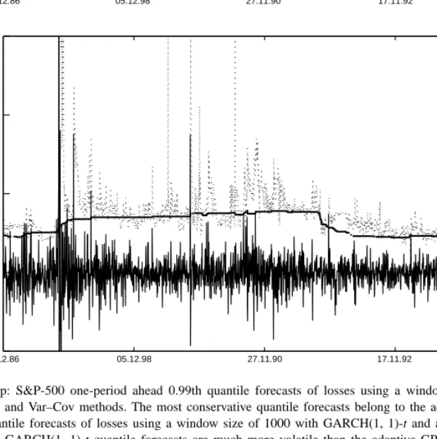
Fig. 9. Top: S&P-500 one-period ahead 0.99th quantile forecasts of losses using a window size of 1000 with adaptive GPD, historical simulation and Var–Cov methods. The most conservative quantile forecasts belong to the adaptive GPD model. Bottom: one-period ahead 0.99th quantile forecasts of losses using a window size of 1000 with GARCH(1, 1)-t and adaptive GPD methods. It is apparent from the figure that GARCH(1, 1)-t quantile forecasts are much more volatile than the adaptive GPD model. Although the GARCH(1, 1)-t model provides more precise forecasts of this quantile, the excessive volatility of the forecasts of the GARCH(1, 1)-t model should be a concern for a risk manager. We restricted the vertical axis to [−0.05, 0.15] to improve the resolution. Otherwise GARCH quantile forecasts are as large as 0.34.
30% which is quite costly to implement and difficult to supervise in practice. The findings from the left tail are parallel to the ones from the ISE-100 analy-sis. In the top panel of Fig. 9quantile forecasts for the Var–Cov, historical simulation and adaptive GPD
354 R. Gençay et al. / Insurance: Mathematics and Economics 33 (2003) 337–356
models are presented. All three models provide rather stable quantile forecasts across volatile return periods. The Var–Cov and historical simulation quantile fore-casts follow similar time paths as the adaptive GPD quantile forecasts.
A comparison between the GARCH(1, 1)-t and adaptive GPD model is presented in the bottom panel of Fig. 9. This comparison indicates that GARCH models yield very volatile quantile estimates when compared to the GPD, historical simulation or Var–Cov approaches. The volatility of the GARCH quantile forecasts are multiples of the GPD quantile forecasts in a number of dates. Based on Fig. 9, the level of change in the GARCH quantile forecasts can be as large as 30% on a daily basis. Our findings from the S&P-500 returns confirm the findings obtained from the ISE-100 returns that the GPD model pro-vides more accurate violation ratios and its quantile forecasts are stable across turbulent times.
From a regulatory point of view, it is important that banks maintain enough capital to protect them-selves against extreme market conditions. This con-cern allows regulators to impose minimum capital requirements in different countries. In 1996, the Basel Committee recommended a framework for measur-ing market risk and credit risk, and for determinmeasur-ing the corresponding capital requirements, see Basel (1996).23 The committee proposes two different ways of calculating the minimum capital risk requirement: a standardized approach and an internal risk man-agement model. In the standardized approach, banks are required to slot their exposures into different supervisory categories. These categories have fixed risk weights set by the regulatory authorities. A bank can utilize its own internal risk management model, subject to approval by the authorities. These models must meet certain conditions. Our “violation ratio” above as a criterion for evaluation of different models is basically the Basel Committee criterion for evalu-ating internal risk management models. We showed that this criterion, in combination with volatile
mar-23The New Basel Capital Accord (Basel II) is expected to be finalized by the end of 2003 with implementation to take place in member countries by year-end 2006. According to a recent consultative document by Basel Committee, the new accord sub-stantially changes the treatment of credit risk and introduces an explicit treatment operational risk; seehttp://www.bis.orgfor fur-ther details.
ket conditions, may result in costly implementations, especially if conditional models are employed to measure the risk. The results also indicate that the existing Basel Committee risk measurement and reg-ulatory framework can be improved by incorporating costs of trading, costs of capital adjustments and the amount of losses into the existing criterion to determine minimum capital requirements.
5. Conclusions
Risk management gained importance in the last decade due to the increase in the volatility of financial markets and a desire of a less fragile financial sys-tem. In risk management, the VaR methodology as a measure of market risk is popular with both financial institutions and regulators. VaR methodology benefits from the quality of quantile forecasts. In this study, conventional models such as GARCH, historical sim-ulation and Var–Cov approaches, are compared to EVT models. The six models used in this study can be classified into two groups: one group consisting of GARCH(1, 1) and GARCH(1, 1)-t models which lead to highly volatile quantile forecasts, while the other group consisting of historical simulation, Var–Cov, adaptive GPD and nonadaptive GPD models provide more stable quantile forecasts. In the first group, GARCH(1, 1)-t, while in the second group the GPD model is preferable for most quantiles.
Our results suggest further study by constructing a cost function that penalizes the excessive volatility and rewards the accuracy of the quantile forecasts at the same time. The results also indicate that the exist-ing Basel committee risk measurement and regulatory framework can be improved by incorporating costs of trading, costs of capital adjustments and the amount of losses into existing criterion to determine minimum capital requirements.
Acknowledgements
Ramazan Gençay gratefully acknowledges financial support from the Swiss National Science Foundation under NCCR–FINRISK, Natural Sciences and Engi-neering Research Council of Canada and the Social Sciences and Humanities Research Council of Canada.
References
Basel, 1996. Overview of the Amendment to the Capital Accord to Incorporate Market Risk. Basel Committee on Banking Supervision, Basel.
Bera, A., Jarque, C., 1981. Efficient tests for normality, hetero-scedasticity and serial independence of regression residuals: Monte Carlo evidence. Economics Letter 7, 313–318. Bollerslev, T., 1982. Generalized autoregressive conditional
heteroscedasticity. Journal of Econometrics 31, 307–327. Boothe, P., Glassman, P.D., 1987. The statistical distribution of
exchange rates. Journal of International Economics 22, 297– 319.
Dacorogna, M.M., Pictet, O.V., Müller, U.A., de Vries, C.G., 2001a. Extremal forex returns in extremely large datasets. Extremes 4, 105–127.
Dacorogna, M.M., Gençay, R., Müller, U.A., Olsen, R.B., Pictet, O.V., 2001b. An Introduction to High-frequency Finance. Academic Press, San Diego, CA.
Danielsson, J., de Vries, C.G., 1997. Tail index and quantile estimation with very high frequency data. Journal of Empirical Finance 4, 241–257.
Danielsson, J., de Vries, C.G., 2000. Value-at-risk and extreme returns. Annales D’Economie et de Statistique 60, 239–270. Danielsson, J., Moritomo, J., 2000. Forecasting extreme financial
risk: a critical analysis of practical methods for the Japanese market. Monetary Economic Studies 12, 25–48.
de Haan, L., Jansen, D.W., Koedijk, K.G., de Vries, C.G., 1994. Safety first portfolio selection, extreme value theory and long run asset risks. In: Galambos, J., Lechner, J., Kluwer, E.S. (Eds.), Extreme Value Theory and Applications. Kluwer Academic Publishers, Dordrecht, pp. 471–488.
Dowd, K., 1998. Beyond Value-at-Risk: The New Science of Risk Management. Wiley, Chichester, UK.
Duffie, D., Pan, J., 1997. An overview of value-at-risk. Journal of Derivatives 7, 7–49.
Embrechts, P., 1999. Extreme value theory in finance and insurance. Department of Mathematics, ETH, Swiss Federal Technical University.
Embrechts, P., 2000a. Extreme value theory: potentials and limitations as an integrated risk management tool. Derivatives Use, Trading and Regulation 6, 449–456.
Embrechts, P., 2000b. Extremes and Integrated Risk Management. Risk Books and UBS Warburg, London.
Embrechts, P., Kluppelberg, C., Mikosch, C., 1997. Modeling Extremal Events for Insurance and Finance. Springer, Berlin. Embrechts, P., Resnick, S., Samorodnitsky, G., 1999. Extreme
value theory as a risk management tool. North American Actuarial Journal 3, 30–41.
Engle, R.F., 1982. Autoregressive conditional heteroscedastic models with estimates of the variance of United Kingdom inflation. Econometrica 50, 987–1007.
Ertuˇgrul, A., Selçuk, F., 2001. A brief account of the Turkish economy: 1980–2000. Russian East European Finance Trade 37, 6–28.
Gençay, R., Selçuk, F., 2001. Overnight borrowing, interest rates and extreme value theory. Department of Economics, Bilkent University.
Gençay, R., Selçuk, F., Ulugülyaˇgcı, A., 2003. EVIM: a software package for extreme value analysis in Matlab. Studies in Nonlinear Dynamics and Econometrics 5, 213–239.
Ghose, D., Kroner, K.F., 1995. The relationship between GARCH and symmetric stable distributions: finding the source of fat tails in the financial data. Journal of Empirical Finance 2, 225– 251.
Hauksson, H.A., Dacorogna, M., Domenig, T., Müller, U., Samorodnitsky, G., 2001. Multivariate extremes, aggregation and risk estimation. Quantitative Finance 1, 79–95.
Hols, M.C., de Vries, C.G., 1991. The limiting distribution of extremal exchange rate returns. Journal of Applied Econo-metrics 6, 287–302.
Jorion, P., 1997. Value-at-Risk: The New Benchmark for Controlling Market Risk. McGraw-Hill, Chicago.
Koedijk, K.G., Schafgans, M.M.A., de Vries, C.G., 1990. The tail index of exchange rate returns. Journal of International Economics 29, 93–108.
Levich, R.M., 1985. Empirical studies of exchange rates: price behavior, rate determination and market efficiency. Handbook of Economics 6, 287–302.
Loretan, M., Phillips, P.C.B., 1994. Testing the covariance stationary of heavy-tailed time series. Journal of Empirical Finance 1, 211–248.
Lux, T., 1996. The stable Paretian hypothesis and the frequency of large returns: an examination of major German stocks. Applied Financial Economics 6, 463–475.
Mandelbrot, B., 1963a. New methods in statistical economics. Journal of Political Economy 71, 421–440.
Mandelbrot, B., 1963b. The variation of certain speculative prices. Journal of Business 36, 394–419.
Mantegna, R.N., Stanley, H.E., 1995. Scaling behavior in the dynamics of an economic index. Nature 376, 46–49. McNeil, A.J., 1997. Estimating the tails of loss severity
distributions using extreme value theory. ASTIN Bulletin 27, 1117–1137.
McNeil, A.J., 1998. Calculating quantile risk measures for financial time series using extreme value theory. Department of Mathematics, ETH, Swiss Federal Technical University, ETH E-Collection.http://e-collection.ethbib.ethz.ch/.
McNeil, A.J., 1999. Extreme value theory for risk managers. Internal Modeling CAD II, Risk Books, pp. 93–113. McNeil, A.J., Frey, R., 2000. Estimation of tail-related risk
measures for heteroscedastic financial time series: an extreme value approach. Journal of Empirical Finance 7, 271–300. Müller, U.A., Dacorogna, M.M., Pictet, O.V., 1998. Heavy tails
in high-frequency financial data. In: Adler, R.J., Feldman, R.E., Taqqu, M.S. (Eds.), A Practical Guide to Heavy Tails: Statistical Techniques for Analysing Heavy Tailed Distributions. Birkhäuser, Boston, pp. 55–77.
Mussa, M., 1979. Empirical regularities in the behavior of exchange rates and theories of the foreign exchange market. In: Carnegie-Rochester Conference Series on Public Policy, pp. 9–57.
Nelson, D.B., 1991. Conditional heteroskedasticity in asset returns: a new approach. Econometrica 59, 347–370.
Pictet, O.V., Dacorogna, M.M., Müller, U.A., 1998. Hill, bootstrap and jackknife estimators for heavy tails. In: Taqqu, M.S.
356 R. Gençay et al. / Insurance: Mathematics and Economics 33 (2003) 337–356 (Ed.), A Practical Guide to Heavy Tails: Statistical Techniques
for Analysing Heavy Tailed Distributions. Birkhäuser, Boston, pp. 283–310.
Reiss, R., Thomas, M., 1997. Statistical Analysis of Extreme Values. Birkhäuser, Basel.
Sullivan, R., Timmermann, A., White, H., 2001. Dangers of data-driven inference: the case of calendar effects in stock returns. Journal of Econometrics 105, 249–286.
Teugels, J.B.J., Vynckier, P., 1996. Practical Analysis of Extreme Values. Leuven University Press, Leuven.