A Higher-Order Sensitive Finite Differences Scheme Of The Cauchy Problem For 2D Linear Hyperbolic Equations With Constant Coefficients In A Class Of Discontinuous Functions

6

BEYKENT ÜNİVERSİTESİ FEN VE MÜHENDİSLİK BİLİMLERİ DERGİSİ CİLT SAYI:13/1

www.dergipark.gov.tr

A HIGHER-ORDER SENSITIVE FINITE DIFFERENCES SCHEME OF THE

CAUCHY PROBLEM FOR 2D LINEAR HYPERBOLIC EQUATIONS WITH

CONSTANT COEFFICIENTS IN A CLASS OF

DISCONTINUOUS FUNCTIONS

Öykü YENER*, Bahaddin SİNSOYSAL**, Mahir RASULOV***

ABSTRACT

In this study we develop a finite difference scheme for practical calculation of the Cauchy problem for the 2D scalar advection equation with a higher accuracy order constant coefficient, encountered in different fields of hydrodynamics. For this aim, to develop an auxiliary problem having some advantages over the main problem is introduced. The proposed auxiliary problem permits us to construct a higher-order sensitive finite differences scheme.

Keywords: Modelling equations of hydrodynamics, Weak solution in a class of discontinuous functions, Moving network

*Makale Gönderim Tarihi: 12.05.2020 ; Makale Kabul Tarihi : 05.06.2020 Makale Türü: Araştırma DOI: 10.20854/bujse.736345 *Sorumlu yazar: Beykent University, Institute of Graduate Studies, PhD Student in Applied Mathematics Department, Taksim, Istanbul, Turkey (yeneroyku@gmail.com) (ORCID ID: 0000-0002-9583-714X)

**Beykent University, Department of Management Information Systems, Sarıyer, Istanbul, Turkey (bsinsoysal@beykent.edu.tr) (ORCID ID: 0000-0003-2926-2744)

***Baku State University, Department of Numerical Methods of Mathematics, Baku, Azerbaijan (mresulov@gmail.com) (ORCID ID: 0000-0002-8393-2019)

SABİT KATSAYILI İKİ BOYUTLU LİNEER HİPERBOLİK DENKLEMLER

İÇİN CAUCHY PROBLEMİNİN SÜREKSİZ FONKSİYONLAR SINIFINDA

YÜKSEK MERTEBEDEN HASSAS SONLU FARKLAR ŞEMASI

Öykü YENER*, Bahaddin SİNSOYSAL**, Mahir RASULOV***

ÖZ

Bu çalışmada, hidrodinamiğin çeşitli alanlarında karşılaşılan iki boyutlu skaler adveksiyon denklemi için yazılmış Cauchy probleminin pratik hesaplanması için bir sonlu fark şeması geliştirilmiştir. Bu amaçla, ana probleme göre bazı avantajları olan bir yardımcı problem sunulmuştur. Önerilen yardımcı problem, daha yüksek mertebeden hassas bir sonlu farklar şeması oluşturmaya imkan sağlar.

Anahtar Kelimeler: Hidrodinamiğin model denklemleri, Süreksiz fonksiyonlar sınıfında zayıf çözüm, Hareketli ağ

*Makale Gönderim Tarihi: 12.05.2020 ; Makale Kabul Tarihi : 05.06.2020 Makale Türü: Araştırma DOI: 10.20854/bujse.736345 *Sorumlu yazar: Beykent University, Institute of Graduate Studies, PhD Student in Applied Mathematics Department, Taksim, Istanbul, Turkey (yeneroyku@gmail.com) (ORCID ID: 0000-0002-9583-714X)

**Beykent University, Department of Management Information Systems, Sarıyer, Istanbul, Turkey (bsinsoysal@beykent.edu.tr) (ORCID ID: 0000-0003-2926-2744)

***Baku State University, Department of Numerical Methods of Mathematics, Baku, Azerbaijan (mresulov@gmail.com) (ORCID ID: 0000-0002-8393-2019)

8

As usual, let R^3 (x,y,t) be Euclidean space of the points (x,y,t) and Q ={a≤x≤b,c≤y≤d}, Q_T=Q×[0,T). Here (x,y) and t are spatial and time variables respectively. In we consider the following problem

Here, A and B are given constants, u0 (x,y) is a known function having in Q some lines of discontinuity of the first type. Equation of the type (1) appears in different model problems of hydrodynamics [1],[3],[4],[6],[7],[8],[15]-[18].

The problem (1), (2) later on we will call the main problem. Let Q_ be the domain defined as follows, Figure 1.

2. Exact Solutions of the Main and Auxiliary Problems

Using the method of characteristics, we can show that the function

is the exact solution of the main problem.

Definition 1. The function u(x,y,t) satisfying the initial condition (2) is called a weak solution of the problem (1),(2) if the following integral relation

holds for every test function φ(x,y,t) defined and is differentiable in the upper half plane and vanishes for the large |x| + t and (x,T) = 0.

Figure 1: The Q_xy domain

Theorem 1. If the function u(x,y,t) is a continuous solution of the main problem, then the function u(x,y,t)= (x-At,y-Bt) is a soft solution of the main problem too, [9].

Proof. According to the definition of the weak solution we have

Theorem 2. If the function u(x,y,t) = (x-At,y-Bt) is integrable, then the function u(x,y,t) is a weak solution of the main problem, [9].

Proof. According to the definition of a weak solution we have

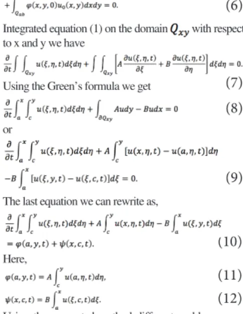
Integrated equation (1) on the domain with respect to x and y we have

Using the Green’s formula we get or

The last equation we can rewrite as,

Here,

Using the suggested method different problems were solved. [10]-[13] The general scheme offered method is shown in Figure 2. The equation (10) together with the condition (2) is called as first auxiliary problem. We introduce the following operator

and the function is defined as

It is easily seen that the function φ(a,y,t)+φ(x,b,t)φkerI. Indeed,

(1)

(2)

(3)

(4)

(10)

(11)

(12)

(14)

(13)

(5)

(6)

(8)

(9)

(7)

Figure 2: The general scheme of the suggested method Sometimes happen conveniently introduce of the second type auxiliary problem defined as follows. Taking into consideration (14) the equation (10) take the form From (14) we have

Indeed, if we differentiate the relation (14) at first with respect to x, then with respect to y we prove the validity of (16).

The initial condition for the equation (15) is

here, the function (x,y) is any continuously differentiable solution of the equation

The problem (15),(17) is called the second type auxiliary problem. Both auxiliary problems have the following advantages:

• The differentiability property of the function v(x,y,t) with respect to x and y is one order higher than u(x,y,t) • The function u(x,y,t) may be discontinuous. • In obtaining the solution u(x,y,t) of the problem (1), (2), we do not use the derivatives u_x, u_y, u_t which can not exist usually.

It is obvious that the solution of the auxiliary problem is not unique [7],[16]. The following theorem is valid. Theorem 3. If the function v(x,y,t) is the classical solution of the auxiliary problem (15),(17), then the function u(x,y,t) defined by (16) is a weak solution of the main problem.

Proof. Let the function φ(x,y,t) be a test function and we consider the following expression

After some simple manipulation we get

Integrating (15) with respect to t, x, y It proves Theorem 3.

Now we introduce a function v(x,y,t) defined by the following relation

Here,

It easily shows that

According to equation (21) we can rewrite equation (10) in the form

Taking into consideration (21) we have Then equation (22) takes the form (15) The exact solution of the problem (15), (17) is 3. Finite Differences Scheme for Cauchy Problem in a Class of Discontinuous Functions

In this section, we intend to introduce the numerical method for the problem (1), (2), and investigate some properties of it. By using the advantages of the suggested auxiliary problem, a new numerical algorithm is proposed. In [10],[11] the suggested numerical method applied to solve for nonlinear scalar equations of hydrodynamics

In further research, we will exploit the concept and theory of finite differences from the familiar books [2],[5],[14],[15]. In order to construct the method, the domain definition of the problem is covered by the following grid,

where, hx, hy and are steps of the grid with respect to x, y and t, respectively. The problem (15),(17) at any points of the grid is approximated by the following differences scheme

The initial condition for (25) is

If we write the equation (25) in point (i-1,j) and subtract it from (25) and divide it by hx we get.

It is easily seen that the function defined with the help of the equality

(16)

(17)

(18)

(21)

(22)

(23)

(24)

(25)

(26)

(27)

(15)

(19)

(20)

10

To approximate of the problem (10),(2) by the finite difference, the integrals leaving into (10) are approximated as follows

and

Taking this into consideration (25)-(27), the equation (9) at any point (i,j,k) of the grid is approximated as follows

The initial condition for (31) is 4. Numerical Experiments

The basic goal of this study is to develop an algorithm for the solution of the Cauchy problem for the 2D parabolic type equation in a class of discontinuous functions. At first this algorithm is tested on a linear equation, and later this method will be developed to a nonlinear problem. Here and later on we will use the advantages of the suggested auxiliary problem. In order to convince on the validity of the suggested method at first the computer tests will be carried out for the exact solution.

For this aim as the function u_0 (x,y), we take

For the sake of simplicity, we assume that A=B=1. There are two cases: (i) u_1>u_2, u_1<u_2. The graphs of these functions are demonstrated in Figure 3a) and 3b).

Figure 3:

a) The graph of the function u_0 (x,y), u_1>u_2; b) The graph of the function u_0 (x,y), u_1<u_2 The initial function of v_0 (x,y) obtained from equation (18)

(28)

(29)

(30)

(31)

(32)

Figure 4:

a) The graph of the function v_0 (x,y), u_1>u_2; b) The graph of the function v_0 (x,y), u_1<u_2 As it is seen from Figure 4a) and 4b) the order of differentiability of v_0 (x,y) is greater than u_0 (x,y), that permits us to apply classical methods. In order to find the exact solution of the main problem, we will use the solution of the auxiliary problem (15),(17) which is expressed as follows:

The graph of the function v(x,y,t) are depicted in Figure 5a) and 5b). Applying the formula (16) we find solution of the main problem Figure 6a) and 6b).

Figure 5:

a) The graph of the function v(x,y,t), u_1>u_2 at T=1; b) The graph of the function v(x,y,t), u_1<u_2 at T=1

Figure 6:

a) The graph of the function u(x,y,t)=Iv(x,y,t), u_1>u_2 at T=1; b) The graph of the function u(x,y,t)=I(x,y,t), u_1<u_2 at T=1 5. Conclusion

An algorithm to calculate the exact solution of the Cauchy problem for the 2D parabolic type equation in a class of discontinuous functions is suggested.

12

[1] Ames W. F. (1965), Nonlinear Partial Differential Equations in Engineering, Academic Press, New York, London.

[2] Ames W. F. (1977), Numerical Methods for Partial Differential Equations, Academic Press, New York.

[3] Anderson D. A., Tannehill J. C., Pletcher R. H. (1984), Computational Fluid Mechanics and Heat Transfer, Vol. 1,2, Hemisphere Publishing Corporation.

[4] Fritz J. (1986), Partial Differential Equations, Springer-Verlag, New York, Heidelberg, Berlin. [5] Godunov S. K., Ryabenkii V. S. (1972), Finite Difference Schemes, Moskow, Nauka. [6] Godunov S. K. (1979), Equations of Mathematical Physicis, Nauka, Moskow.

[7] Goritskii A. A., Krujkov S. N., Chechkin G. A. (1997), A First Order Ouasi-Linear Equations with Partial Differential Derivaites, Pub. Moskow University, Moskow.

[8] Leveque R. J. (2002), Finite Volume Methods for Hyperbolic Problems, Cambridge University Press, 558p.

[9] Noh W. F., Protter M. N. (1963), “Difference Methods and the Equations of Hydrodynamics”, Journal of Math. and Mechanics, 12(2).

[10] Rasulov M. A. (1991), “On a Method of Solving the Cauchy Problem for a First Order Nonlinear Equation of Hyperbolic Type with a Smooth Initial Condition”, Soviet Math. Dok., 43 (1).

[11] Rasulov M. A., Ragimova, T. A. (1992), “A Numerical Method of the Solition of ne Nonlinear Equation of a Hyperbolic Type of the First Order Differential Equations”, Minsk, 28(7), 2056-2063. [12] Rasulov M. A. (1991), “Identification of the Saturation Jump in the Process of Oil Displacement by Water in a 2D Domain”, Dokl RAN, 319(4), 943-947.

[13] Rasulov M. A., Coskun E., Sinsoysal B. (2003), “Finite Differences Method for a Two-Dimensional Nonlinear Hyperbolic Equations in a Class of Discontinuous Functions”, App. Mathematics and Computation, vol.140, Issue l, August, pp.279-295, USA.

[14] Richmyer R. D., Morton K. W. (1967), Difference Methods for Initial Value Problems, New York, Wiley, Int.

[15] Samarskii A. A. (1977), Theory of Difference Schemes, Moskow, Nauka.

[16] Smoller J. A. (1983), Shock Wave and Reaction Diffusion Equations, Springer-Verlag, New York Inc.

[17] Toro E. F. (1999), Riemann Solvers and Numerical Methods for Fluid Dynamics, Springer-Verlag, Berlin Heidelberg.

[18] Whitham G. B. (1974), Linear and Nonlinear Waves, Wiley Int., New York.

BEYKENT ÜNİVERSİTESİ FEN VE MÜHENDİSLİK BİLİMLERİ DERGİSİ CİLT SAYI:13/1