A parallel scaled
conjugate-gradient
algorithm for the solution
phase of gathering
radiosity on hypercubes
Tahsin M. Kuri, Cevdet Aykanat,
Bu¨lent O®zgu¨i
Department of Computer Engineering and Informa-tion Science, Bilkent University, 06533, Bilkent, An-kara, Turkey
Gathering radiosity is a popular method for investigating lighting effects in a closed environment. In lighting simulations, with fixed locations of objects and light sour-ces, the intensity and color and/or reflec-tivity vary. After the form-factor values are computed, the linear system of equa-tions is solved repeatedly to visualize these changes. The scaled conjugate-gradient method is a powerful technique for solving large sparse linear systems of equations with symmetric positive definite matrices. We investigate this method for the solution phase. The nonsymmetric form-factor matrix is transformed into a symmetric matrix. We propose an efficient data redistribution scheme to achieve almost perfect load balance. We also present several parallel algorithms for form-factor computation.
Key words: Gathering radiosity — Scaled conjugate-gradient method — Parallel al-gorithms — Hypercube multicomputer — Data redistribution
Correspondence to: T.M. Kuri
1 Introduction
Realistic synthetic image generation by com-puters has been a challenge for many years in the field of computer graphics. It requires the accurate calculation and simulation of light propagation and global illumination effects in an environment. The radiosity method (Goral et al. 1984) is one of the techniques for simulating light propagation in a closed environment. Radiosity accounts for the diffuse inter-reflections between the surfaces in a diffuse environment. There are two approaches to radiosity: progressive refinement (Cohen et al. 1988) and gathering. Gathering is a very suitable approach for investigating lighting effects within a closed environment. For such applications, the locations of the objects and light sources in the scene usually remain fixed, while the intensity and color of light sources and/or reflectivity of surfa-ces change in time. The linear system of equations is solved many times to investigate the effects of these changes. Therefore, efficient implementation of the solution phase is important for such applications.
Although gathering is excellent for some applica-tions in realistic image generation, it requires much computing power and memory storage to hold the scene data and computation results. As a result, applications of the method on conven-tional uniprocessor computers for complex envi-ronments can be far from practical due to high computation and memory costs. Distributed memory multicomputers, however, can provide a cost-effective solution to problems that require much computation power and memory storage. In these types of architectures, processors are con-nected to other processors by an interconnection network, such as a hypercube, ring, mesh, etc. Data are exchanged and processors are synchro-nized via message passing.
Various parallel approaches have been proposed and implemented for gathering radiosity (Chal-mers and Paddon 1989, 1990; Price and Truman 1990; Paddon et al. 1993). In these approaches, the Gauss—Jacobi (GJ) method is used in the solution phase. The scaled conjugate-gradient (SCG) method is known to be a powerful technique for the solution of large sparse linear systems of equa-tions with symmetric positive definite matrices. In general, the SCG method converges much faster than the GJ method. In this work, the utilization and parallelization of the SCG method is investi-gated for the solution phase. The nonsymmetric
form-factor matrix is efficiently transformed into a symmetric matrix. An efficient data redis-tribution scheme is proposed and discussed to achieve an almost perfect load balance in the solution phase. Several parallel algorithms for the form-factor computation phase are also presented.
The organization of the paper is as follows. Sec-tion 2 describes the computaSec-tional requirements and the methods used in the form-factor compu-tation and solution phases. The GJ and SCG methods for the solution phase are described in this section. Section 3 briefly summarizes the existing work on the parallelization of the radio-sity method. Section 4 briefly describes the hy-percube multicomputer. Section 5 presents the parallel algorithms for form-factor computation. The parallel algorithms developed for the solution phase are presented and discussed in Sect. 6. Load balancing in the solution phase and a data redis-tribution scheme are discussed in Sect. 7. Finally, experimental results from a 16-node Intel iPSC/2 hypercube multicomputer are presented and dis-cussed in Sect. 8.
2 Gathering radiosity
In the radiosity method, every surface and object constituting the environment is discretized into small patches, which are assumed to be perfect diffusers. The algorithm calculates the radiosity value of each patch in the scene.
The gathering radiosity method (the term
radio-sity method will also be used interchangeably
to refer to the gathering method) consists of three successive computational phases: the form-factor computation phase, the solution phase,
and the rendering phase. The form-factor
matrix is computed and stored in the first phase. In the second phase, a linear system of equations is formed and solved for each color band (e.g., red, green, blue) to find the radiosity values of all patches for these colors. In the last phase, results are rendered and displayed on the screen. They are derived from the radiosity values of the patches computed in the second phase. Conventional rendering methods (Watt 1989; Whitman 1992) (e.g., Gouraud shading, Z-buffer algorithm) are used in the last phase to display the results.
This section describes the computational require-ments and the methods used in the form-factor computation and solution phases.
2.1 Form-factor computation phase
In an environment discretized into N patches, the radiosity bi of each patch ‘i’ is computed as follows:
bi"ei#ri +N
j/1bjFij
(1)
where ei and ri denote the initial radiosity and reflectivity values, respectively, of patch ‘i ’, and
the form-factor Fij denotes the fraction of lightthat leaves patch ‘j’ and is incident on patch ‘i’.
The Fij values depend on the geometry of the scene, and they remain fixed as long as the ge-ometry of the scene remains unchanged. The
Fii values are taken to be zero for convex patches.An approximation method to calculate the form
factors, called the hemicube method, is proposed by Cohen and Greenberg (1985). In this method, a discrete hemicube is placed around the center of each patch. Each face of the hemicube is divided into small squares (surface squares). A typical
hemicube is composed of 100]100]50 such
squares. Each square ‘s’ corresponds to a delta
form-factorDf (s).
After allocating a hemicube over a patch ‘i’, all other patches in the environment are projected onto the hemicube for hidden patch removal. Then, each square ‘s’ allocated by patch ‘j’
con-tributes Df (s) to the form-factor Fij between
patches ‘i’ and ‘j’. At the end of this process, the
ith row of the form-factor matrix F is constructed.
The F matrix is a sparse matrix because a patch may not see all the patches in the environment due to the occlusions. In order to reduce the memory requirements, space is allocated dynam-ically for only nonzero elements of the matrix during the form-factor computation phase. Each element of a row of the matrix is in the form [column id, value]. (This compressed form requires 8 bytes for each nonzero entry, 4 bytes for the
column-id, and 4 bytes for the value. We observed
that +30% of the matrix entries are nonzero in our test scenes. Hence, for N patches,
approximately 2.4N2 bytes are required to store the F matrix.) The column id indicates the j index of an Fij value in the ith row.
2.2 Solution phase
In this phase, the linear system of equations of the form
Cb"(I!RF)b"e (2)
is solved for each color band. Here, R is the diagonal reflectivity matrix, b is the radiosity vec-tor to be calculated, e is the vecvec-tor representing the self-emission (initial emission) values of patches, and F is the form-factor matrix.
Methods for solving such a linear system of equa-tions can be grouped as direct methods and iter-ative methods (Golub and van Loan 1989). In this work, iterative methods have been used in the solution phase because they exploit and preserve the sparsity of the coefficient matrix. In addition, unlike direct methods, maintaining only F is suffi-cient in the formulation of iterative methods in this work. Hence, they require less storage than direct methods. Furthermore, iterative methods are more suitable for parallelization. It has been experimentally observed that iterative methods converge quickly to acceptable accuracy values. Three popular iterative methods widely used for solving linear system of equations are the Gauss—Jacobi (GJ), Gauss—Seidel (GS), and con-jugate-gradient (CG) methods (Golub and van Loan 1989). The GS scheme is inherently sequen-tial; hence, it is not suitable for parallelization. Thus, only the GJ and CG schemes are described and investigated for parallelization in this work.
2.2.1 The GJ method
In the GJ method, the iteration equation for the solution phase of the radiosity becomes
bk`1"RFbk#e. (3)
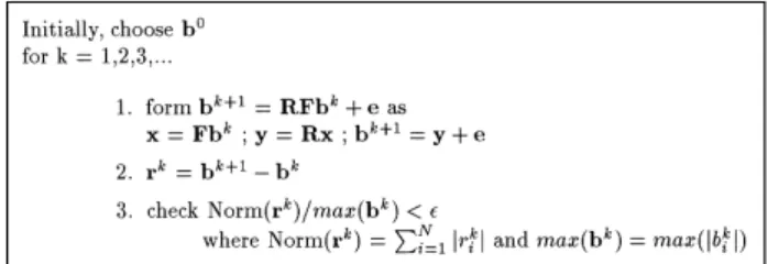
Note that it suffices to store only the diagonals of the diagonal R matrix. Hence, matrix and vector will be used interchangeably to refer to a diagonal matrix. The GJ algorithm necessitates storing
Fig. 1. Basic steps of the GJ method
only the original F matrix and the reflectivity vector for each color in the solution phase. The algorithm for the GJ method is given in Fig. 1. The computational complexity of an individual GJ iteration is:
¹GJ+(2M#6N)tcalc (4)
where M is the total number of nonzero entries in the F matrix, and N is the number of patches in the scene. Here, scalar addition, multiplication, and absolute value operations are assumed to take the same amount of time tcalc.
2.2.2 The SCG method
The convergence of the CG method (Hestenes and Stiefel 1952) is guaranteed only if the coefficient matrix C is symmetric and positive definite. How-ever, the original coefficient matrix is not symmet-ric since cij"riFijOrjFji"cji. Therefore, the CG method cannot be used in the solution phase using the original C matrix as is also mentioned by Paddon et al. (1993). However, the reciprocity relation AiFij"AjFji between the form-factor values of the patches can be exploited to trans-form the original linear system of equations in Eq. 2 into
Sb"De (5)
with a symmetric coefficient matrix S"DC where D is a diagonal matrix D"diag[A1/r1,
A2/r2,2, AN/rN]. Note that matrix S is
symmet-ric since sij"AiFij"AjFji"sji for jOi. The ith row of the matrix S has the following structure:
Si*"[!AiFi1,2, !AiFi,i~1, Ai/ri,
!
for i"1, 2,2, N. Therefore, matrix S preserves diagonal dominance. Thus, the coefficient matrix S in the transformed system of equations (Eq. 5) is positive definite since diagonal dominance of a matrix ensures its positive definiteness, which is also shown by Neumann (1994, 1995) indepen-dently of our work.
The convergence rate of the CG method can be improved by preconditioning. In this work, simple yet effective diagonal scaling is used for preconditioning the coefficient matrix S. In this preconditioning scheme, rows and columns of the coefficient matrix S are individually scaled by the diagonal matrix D"diag[A1/r1,2, AN/rN]. Hence, the CG algorithm is applied to solve the following linear system of equations
S3 b3"e8 (6)
where S3 "D~1@2SD~1@2"D~1@2DCD~1@2"
D1@2CD~1@2 has unit diagonals, b3"D1@2b, and
e8 "D~1@2De"D1@2e. Thus, the vector De on the
right-hand side in Eq. 5 is also scaled, and b3 must
be scaled back at the end to obtain the original
solution vector b (i.e., b"D~1@2b3). The
eigen-values of the scaled coefficient matrix S3 (in Eq. 6)
are more likely to be grouped together than those of the unscaled matrix S (in Eq. 5), thus resulting in a better condition number.
The entries of the scaled coefficient matrix S3 are of
the following structure:
sJ ij"
G
!Jdiicij 1 Jdjj"!S
Airi riFijS
Ajrj "!JriAiS
rj AjFij if iOj 1 otherwise.The values of the scaling parameters JriAi and
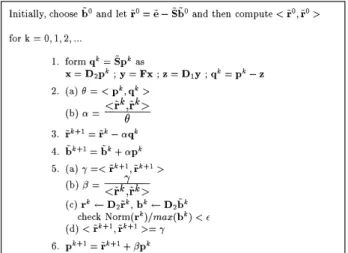
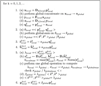
Jrj/Aj depend only on the area and reflectivity values of the patches and do not change through-out the iterations. Therefore, the values of the scaling parameters can be computed once at the beginning of the solution phase and maintained in two vectors (for each color band) representing two diagonal matrices D1"diag[Jr1A1,2, JrNAN] and D2"diag[Jr1/A1,2,JrN/AN]. The basic steps of the SCG algorithm proposed
Fig. 2. Basic steps of the SCG method
for the solution phase of the radiosity method is
illustrated in Fig. 2. The pk and r8k-vectors in
Fig. 2 denote the direction and residual vectors at
iteration k, respectively. Note that r8 k"e8!S3b3k
must be null when b3 k is coincident with the
solu-tion vector.
The matrix vector product qk"S3pk looks as if the
S3 matrix is to be computed and stored for each
color band. However, this matrix vector product can be rewritten for each color as:
qk(r, g, b)"S3(r, g, b)pk(r, g, b)
"
[I!D1(r, g,b)FD2(r, g, b)]pk(r, g, b)
"pk(r, g, b)!D1(r,g,b)FD2(r,g,b)
]pk(r, g, b). (7)
Hence, it suffices to compute and store only the original F matrix and two scaling vectors D1 and D2 for each color band for the SCG method. However, in order to minimize the computational overhead during iterations due to this storage scheme, the vector D1FD2pk should be computed as a sequence of three matrix vector products, x"D2pk, y"Fx and z"D1y, which take H(N), H(M) and H(N) times, respectively. Since
M"O(N2), the computational overhead due to
the diagonal matrix vector products x"D2pk, z"D1x, and the vector subtraction qk"pk!z
computational complexity of a single SCG iter-ation is
¹SCG+(2M#18N)tcalc. (8)
Although the operations shown convert the C matrix into a symmetric matrix, in practice one should be careful when using the SCG method. The hemicube method used in the form-factor calculations is an approximation. As a result, the form-factor values calculated may contain nu-meric errors due to the violation of some assump-tions (Baum et al. 1989). Therefore, the reciprocity relation may not hold, and the operations may still result in a nonsymmetric matrix.
2.2.3 Convergence check
The convergence of iterative methods is usually checked by comparing a selected norm of the
residual error vector rk"e!Cbk with a
prede-termined threshold value at each iteration k. In this work, the following error norm is used for the convergence check:
Errork"+Ni/1DrkiD
max(DbkiD), (9)
where D · D denotes the absolute value. Iterations
are terminated when the error becomes less than
a predetermined threshold value (e.g., errork(e
wheree"5]10~6). Note that the residual vector
rk is already computed n the SCG method.
How-ever, the residual vector rk is not explicitly
com-puted in the GJ scheme. Nonetheless,
rk"e!Cbk"e!(I!RF)bk
"e#RFbk!bk"bk`1!bk. (10)
Hence, the residual error vector rk can easily be
calculated at each iteration of the GJ scheme by a single vector subtraction operation.
3 Related work
There are various parallel implementations for progressive refinement and gathering methods in
the literature (Chalmers and Paddon 1989, 1990, 1991; Price and Truman 1990; Purgathofer and Zeiller 1990; Feda and Purgathofer 1991; Guitton et al. 1991; Jessel et al. 1991; Drucker and Schroeder 1992; Varshney and Prins 1992; Pad-don et al. 1993; Aykanat et al. 1996). In this section, parallel approaches for the gathering method are summarized.
Price and Truman (1990) parallelize the gathering method on a transputer-based architecture in which the processors were organized as a ring having a master processor, used for communicat-ing with host and graphics system, and had a number of slave processors to do the calcu-lations. Any data can be exchanged with this ring interconnection. In their approach, they assume that total scene data can be replicated in the local memories of the processors, hence form factors can be computed without any interprocessor communication. The GJ iterative scheme is used in their solution phase.
Purgathofer and Zeiller (1990) use a ring of trans-puters. In the form-factor computation phase, ‘‘receiving’’ patches are statically distributed to worker processors. Patches are distributed to pro-cessors randomly to obtain a better load balance. The master processor sends global patch informa-tion in blocks to the first processor in the ring. Then, the patch information is circulated in the ring. In their approach, the sparsity of the form-factor matrix is exploited, and the matrix is main-tained in compressed form. The memory used for matrix rows and hemicube information is over-lapped, allowing the calculation of several rows of the matrix at a time in each processor. The num-ber of rows calculated at a time decreases as more rows allocate memory shared with hemicube information.
Chalmers and Paddon (1989, 1990) use a demand-driven approach in the form-factor computation phase and a data-driven approach in the solution phase in which data are assigned to processors in a static manner. The target architecture is based on transputers arranged in a structure of minimal path lengths. Paddon et al. (1993) discuss the trade-offs between demand and data-driven schemes in the parallelization of the form-factor computation phase. Chalmers and Paddon (1989) address the data redistribution issue for better load balancing in the solution phase. Chalmers
approach for the form-factor calculation phase. The form-factor row computations are concep-tually divided evenly among the processors. The even decomposition here refers to the equal num-ber of row allocations to each conceptual region. Each processor is assigned a task by the master from its conceptual region until all tasks in its region are consumed. Idle processors whose con-ceptual regions are totally consumed are assigned tasks from the conceptual regions of other proces-sors. However, in such cases, the computed form-factor vectors are passed to the processors that own the conceptual region. The GJ iterative scheme is used in the solution phases of all these works.
4 The hypercube multicomputer
Among the many interconnection topologies, the hypercube topology is popular because many other topologies, such as ring and mesh, can be embedded into it. Therefore, it is possible to ar-range processors in the most suitable interconnec-tion topology for the soluinterconnec-tion of the problem.
A d-dimensional hypercube consists of P"2d
processors (nodes) with a link between every pair of processors whose d-bit binary labels differ in one bit. Thus, each processor is connected to
d other processors. The hamming distance between
two processors in a hypercube is defined as the number of different bits between these two proces-sors’ ids. The channel i refers to the communica-tion links between processors whose processor ids differ in only the ith bit.
Intel’s iPSC/2 hypercube is a distributed memory multicomputer. Data are exchanged and synchro-nized between nodes via exchanging messages. In this multicomputer, interprocessor communication time (¹comm) for transmitting m words can be modeled as ¹comm"tsu#mttr, where ttr is the trans-mission time per word, and tsu (Attr in the iPSC/2 hypercube multicomputer) is the set-up time.
5 Computation of the parallel
form-factor matrix
In this section, the parallel algorithms devised for the phase computing the form-factor matrix in the gathering method are described.
5.1 Static assignment
In this scheme, each processor is statically as-signed the responsibility of computing the rows corresponding to a subset of patches prior to the parallel execution of this phase. However, projec-tion computaprojec-tions onto local hemicubes may introduce load imbalance during the parallel form-factor computation phase. The complexity of the projection of an individual patch onto a hemicube depends on several geometric factors. A patch that is clipped completely requires much less computation than a visible patch, since it leaves the projection pipeline in a very early stage. Furthermore, a patch with a large projection area on a hemicube requires more scan-conversion computation than a patch with a small projection area. Hence, the assignment scheme should be carefully selected in order to maintain the load balance in this phase.
In this work, we recommend two types of static assignment schemes: scattered and random. In the scattered assignment scheme, the adjacent patches on each surface are ordered consecutively. Then, the successive patches in the sequence are as-signed to the processors in a round-robin fashion. Note that filling the hemicube for the adjacent patches is expected to take an almost equal amount of computation due to the similar view volumes of adjacent patches. Hence, scattered as-signment is expected to yield a good load balance. The scattered assignment of the patches on a regular surface (e.g., rectangular surface) is trivial. Unfortunately, this assignment scheme may necessitate expensive preprocessing computations for the irregular surfaces. The random assignment scheme is recommended if the scene data are not suitable for the preprocessing needed for the scat-tered assignment scheme. In this assignment scheme, randomly selected patches are similarly assigned to the processor in a round-robin fashion. It has been observed experimentally that the random assignment scheme yields a fairly
good load balance for a sufficiently large NP ratio.
The random assignment scheme is used in this work.
In both of these two assignment schemes, first (N mod P) processors in the decimal processor
or-dering are assignedvNPw patches, whereas the
re-maining processors are assigned xNPy patches.
so thatNP patches assigned to processor l are
re-numbered fromNPl to NP(l#1)!1. The new global
numbering (new patch ids) is not modified throughout the computations.
5.1.1 Patch circulation
In this scheme, the host processor distributes only local path information to node processors. After receiving the local patch information, each pro-cessor calculates the rows of the F matrix for its local patches. Each processor places a hemicube around the center of a local patch and calculates the form-factor row for that patch. Each proces-sor’s local patch information is circulated among the processors so that it can project all patches to their local hemicubes. The ring-embedded hy-percube structure, which can easily be achieved by gray-code ordering (Ranka and Sahni 1990), is used for patch circulation. If the number of patches N is not a multiple of P, those processors
havingvNPw local patches require one more patch
circulation phase than the processors havingxNPy
local patches. Hence, those processors having xNPy patches participate in an extra patch circula-tion phase (which does not include any local hemicube fill operation) for the sake of other processors.
In this scheme, information for H(NP) patches is
concurrently transmitted to successive processors of the ring in each communication step. The total volume of concurrent communication in a single
circulation step is then H(NP)(P!1)"H(N).
Hence, the total concurrent communication
vol-ume is H(N)vNPw"H(N2
P). This communication
overhead can be reduced by avoiding communi-cation as much as possible. To do this, the global patch information is duplicated at each node pro-cessor. The scheme to implement this idea is given in the following section.
5.1.2 Storage sharing scheme
Dynamic memory allocation is used for storing the computed F matrix rows. This scheme can be exploited to share the memory needed for global patch information with the memory to be allo-cated to nonzero matrix elements. With such a sharing of memory, we can avoid interprocessor
communication until the memory allocated to global patch information is required for a row of the matrix.
In this scheme, the global patch information is duplicated in each processor after the local patch assignment and the corresponding global patch renumbering mentioned earlier. Then, processors concurrently compute and store the form-factor rows corresponding to their local assignment. They avoid interprocessor communication until no more memory can be allocated for the new row. If a processor cannot allocate memory space for storing the computed form-factor row, it broadcasts a message so that other processors can switch to the communication phase as soon as possible and run the patch circulation scheme. Note that the patch should be circulated until all remaining rows of the F matrix are calculated. Therefore, the data circulation phase in the patch circulation scheme should be repeated a number of times equal to the maximum number of un-processed patches remaining.
5.2 Demand-driven assignment
This approach is an attempt to achieve better load balance through patch assignment to idle proces-sors upon request. The scheme proposed in this work has similarities to the approach used by Chalmers and Paddon 1989, (1990). However, un-like their scheme, the patches are not divided
conceptually. When a patch is processed, the
com-puted form-factor row remains in the processor. In this scheme, each node processor demands a new patch assignment from the host processor as soon as it computes the form-factor row(s) associated with the previous patch assignment. The host processor sends the necessary informa-tion for a predefined number of patch assignments to the requesting node processor. The number of patch assignments at a time is a factor that affects the performance. The number of node-to-host and host-to-node communications decreases with an increasing number of patch assignments at a time. However, this may affect the quality of load bal-ance adversely.
Each node processor keeps an array to save the reflectivity and emission values of the processed patches. The global ids of the processed patches are also saved in an array to be used in the
solution phase. In addition, each processor holds the information for all patches in the scene to avoid interprocessor communication, as is explained in Sect. 5.1.2. The host processor behaves as a master. It is responsible for processing requests and syn-chronizing nodes between phases. The host pro-gram maintains an array for global patch informa-tion and keeps account of the remaining patches to be processed. All node processors are synchronized by the host processor when one or more of the node memories become full, and processors have to switch to the data circulation mode. The host is also responsible for the termination of the form-factor computation phase.
6 Parallel solution phase
This section describes the parallel GJ and SCG algorithms developed for the solution phase. The parallel implementation of the solution phase is closely related to the schemes used in the phase computing the form-factor matrix because patch distribution, hence row distribution, to the pro-cessors differs in each scheme. In the following sections, parallel algorithms for the solution phase are described. We assume that a static as-signment scheme is used in the phase computing the parallel form-factor. An efficient parallel re-numbering scheme, described in Sect. 6.3, adapts these algorithms if the demand-driven assignment scheme is used in this phase.
6.1 Parallel Gauss
—
Jacobi (GJ) method
The GJ algorithm formulated (Fig. 1) for the solu-tion phase has the following basic types of
opera-tions: matrix vector product (x"Fbk), diagonal
matrix vector product (y"Rx), vector
subtrac-tion/addition (bk`1"y#e, rk"bk`1!bk),
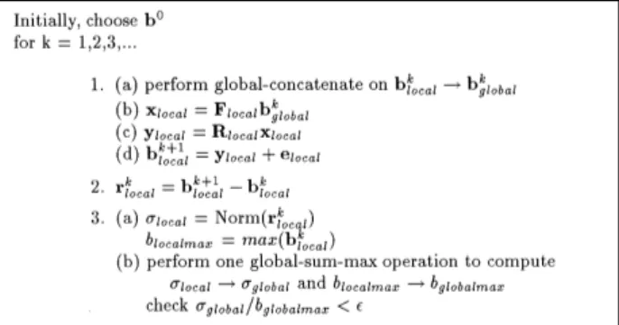
vec-tor norm and maximum (step 3). All of these basic operations can be performed concurrently by dis-tributing the rows of the form-factor matrix F, the corresponding diagonals of the R matrix, and the corresponding entries of the b and e vectors. In the parallel form-factor computation, each processor computes the complete row of form factors for its local patches. Hence, each processor holds a row slice of the form-factor matrix at the end of the form-factor computation phase. Thus, the row
Fig. 3. The parallel GJ algorithm
partitioning required for the parallelization of the solution phase is automatically achieved in this phase. The slices of the R, b, and e vectors are mapped to the processors accordingly. With such a mapping, each processor is responsible for updat-ing the values of those b and r vector elements assigned to it. That is, each processor is responsible for updating its own slice of the global b vector in a local B array (of size N/P) at each iteration. Figure 3 illustrates the parallel GJ algorithm. In an individual GJ iteration, each processor needs to calculate a local matrix vector product
that involves NP inner products of its local rows
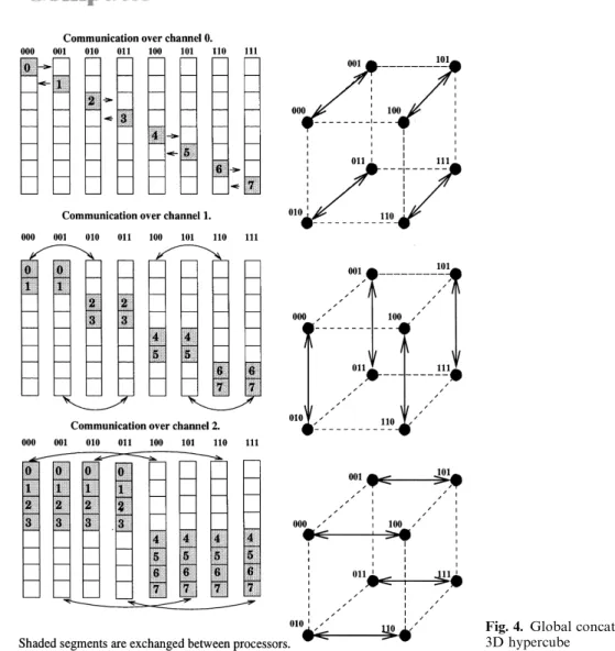
with the global b vector. To do this, the whole b vector computed in a distributed manner in a particular iteration is needed by all processors in the next iteration. This requirement necessitates the global concatenate operation, which is illus-trated for a 3D hypercube topology in Fig. 4. In this operation, each processor l moves its local b array to the lth slice of a working array GB of size N. Then, log2P concurrent exchange com-munication steps are taken between neighbor pro-cessors over channels j"0, 1, 2,2, log2P!1, as is illustrated in Fig. 4. Note that the amount of concurrent data exchange between processors is
only NP in the first step, and it is doubled at each
successive step. That is, at the ith communication step, processors exchange the appropriate slices of
size 2(i~1) NP of their local GB array over channel
i!1. Therefore, the total volume of concurrent
communication is:
Volume of communication"log2+P~1
j/0
2jN
P
"(P!1)N
Fig. 4. Global concatenate operation for a 3D hypercube
The distributed vector add/subtract operations are performed concurrently as local vector
opera-tions on vectors of size NP without necessitating
any interprocessor communication. The partial sums computed by each processor must be added to form the global sum to compute the vector
norm (+Ni/1DriD). In addition, local blocalmax values
should be compared to obtain the global max-imum (bglobalmax). Furthermore, the results should be distributed to all processors in order to ensure the termination at the same iteration. The distrib-uted global norm operation can be performed by a global sum operation. The exchange-communi-cation sequence of the global sum operation is exactly the same as that of global concatenate operation. The only difference is the local scalar
addition after each exchange communication step (Aykanat et al. 1988) instead of the local vector concatenation. This local scalar operation in-volves the addition of the received partial sum to the current partial sum. Similarly, the distributed global maximum can be found by using the
glob-al max operation. The globglob-al max operation can
be done by replacing the local scalar addition operation with a comparison operation in global sum operation. Performing global sum and global max operations successively requires 2log2P of set-up time. Fortunately, this set-up time can be decreased to log2P by combining the global max and global sum operations into a single global operation (global sum-max). In this global operation, partial sums and current maximums
are exchanged after each exchange communica-tion step. Therefore, assuming a perfect load bal-ance, the parallel computational complexity of an individual GJ iteration is:
¹GJ+
A
2MP #6N
P
B
tcalc#2log2Ptsu#
A
P!1P N#2log2P
B
ttr. (12)As is seen from this equation, the communication overhead can be considered negligible for a
sufficiently large granularity (i.e., M/PAN).
Note that this equation is equivalent to Eq. 4 for P"1.
6.2 Parallel scaled conjugate-gradient
(SCG) method
The SCG algorithm (Fig. 2) formulated for the solution phase has the following basic types of operations: matrix-vector product (y"Fx), diag-onal matrix-vector products (x"D2pk, z"D1y),
vector subtraction (qk"pk!z), inner products
(Sr8k, r8kT, Spk, qkT), vector update through
SAXPY operations in steps 3, 4, and 6, and vector norm and maximum operations for the conver-gence check. All of these basic operations can be performed concurrently by distributing the rows of the F matrix and the corresponding entries of the e, D1, D2, x,y, z, b,p, r8, and q vectors.
As is discussed for the parallel GJ algorithm, during the phase of the parallel form-factor com-putation, the rows of the F matrix are assigned to the processors automatically. With such a map-ping, each processor stores its own (local) row slice of the F matrix and the corresponding slices of the e, D1, and D2 vectors. Furthermore, each processor is responsible for updating its local
sli-ces of the x, y, z, b, p, r8 , q vectors. Figure 5
illus-trates the parallel SCG algorithm.
A sequence of distributed matrix and vector com-putations are needed for the distributed
computa-tion of the qk vector. To find the diagonal matrix
vector products x"D2pk and z"D1y, the pro-cessors concurrently compute their local xlocal and zlocal vectors by computing element-by-element products of pairs of local vectors that correspond
Fig. 5. The parallel SCG method
to their slices of the global D2, pk and D1, y vec-tors, respectively. Thus, the distributed diagonal matrix vector product does not necessitate any interprocessor communication. As is the case in the GJ method, the distributed computation of the matrix vector product y"Fx necessitates global concatenation on the local xlocal vector stored in a local array X of size N/P in each processor. Then, the processors concurrently compute their local ylocal vectors by multiplying a local matrix corresponding to their slice of the F matrix with the global xglobal vector, collected in an array GX of size N in their local memories after the global concatenate operation. Finally, the processors concurrently compute their local
qklocal vectors with local vector subtraction
operation.
All processors need the most recently updated
values for the global scalars aglobal and bglobal for
their local vector updates in steps 3, 4, and 6. As is seen in steps 2 and 5, the update of these global scalars involves computing the inner products Sqk, pkT and Sr8k`1, r8k`1T at each iteration. Hence, all processors should receive the results of these distributed inner product computations. To com-pute these products, the processors concurrently compute the local inner products (partial sums) corresponding to their slices of the respective global vectors. Then, the results are accumulated in the local memory of each processor by a glob-al-sum operation. At the end of the global sum
operation, the processors can concurrently
com-pute the same value for the global scalarsaglobal
andbglobal with these global inner product results.
In steps 3, 4, and 6, the processors concurrently update their local blocal, r8local and plocal vectors with local SAXPY operations on these vectors. Note that the distributed norm and maximum opera-tions also necessitate global sum-max operaopera-tions after all processors concurrently compute their local (partial) error norms and maximums, which correspond to the norm/maximum of their sli-ces of the global r and b vectors. Fortunately, these operations and the global inner product Sr8k`1, r8k`1T can be concurrently accumulated in the same global operation to avoid the extra over-head of the log2P set-up time. In this global op-eration, one local maximum and two partial sums are exchanged in each of the log2P concurrent exchange steps. Therefore, assuming a perfect load balance, the parallel computational com-plexity of an individual SCG iteration is:
¹SCG+
A
2MP #18N
P
B
tcalc#3log2Ptsu#
A
P!1P N#4log2P
B
ttr. (13)As is seen from this equation, the communication overhead can be considered negligible for a
suffi-ciently large granularity (i.e., M/PAN).
6.3 A parallel renumbering scheme
In the form-factor computation phase of the static assignment scheme, patches are renumbered and assigned to the node processors so that processor
l has patches from NPl to NP(l#1)!1 for l"0, 1, 2,2, P!1. Therefore, the exchange
sequence, together with the local concatenate scheme in the global concatenate operations at step 1a of the parallel GJ algorithm and step 1b of the parallel SCG algorithm, maintains the orig-inal global patch ordering of the static assignment scheme in the local copies of the global vectors. Hence, during the concurrent local matrix vector products, the appropriate entries in the current global vectors collected in the local GB (in GJ) and GX (in SCG) arrays can be accessed for
multiplication by indexing through the column ids of the local nonzero form-factor values. Unfortu-nately, this nice consistency between the global patch numbering and the global F matrix row ordering among the processors is disturbed in the demand-driven assignment scheme. Hence, the demand-driven assignment scheme necessitates two-level indexing for each scalar multiplication involved in the local matrix vector products at each iteration. We propose an efficient parallel renumbering scheme to avoid this two-level indexing.
During the computation of the form-factor matrix in the demand-driven assignment scheme, each processor saves the global id of the patches it receives from the host processor in a local integer array ID. After the form-factor computation, a global-concatenate operation on these local ar-rays collects a copy of the global GID array in each processor. Note that the collection operation is done in the same way as the global concatenate operation to be performed on the local B (in GJ) and X (in SCG) arrays during the iterations. Hence, there is a one-to-one correspondence between the GB (GX) and GID arrays such that the radiosity value in GB[i] (GX[i]) belongs
to the patch whose original global id"
GID[i]. Then, each processor constructs the same
permutation array PERM of size N, where
PERM[GID[i]]"i (for i"1, 2,2, N) by
per-forming a single for loop. Here, PERM[i] de-notes the new global id for the ith patch in the original global numbering. Then, each processor concurrently updates the column—id values of all its local nonzero form-factor values using
the PERM array as column—id"PERM
[column—id]. Note that this renumbering opera-tion is performed only once as a preprocessing step just before the solution phase, and it is not repeated when the reflectivity and/or emission values are modified.
7 Load balancing in the solution
phase: data redistribution
Assigning equal numbers of F matrix rows and the corresponding vector elements suffices to achieve a perfect load balance during the distrib-uted vector operations involved in the GJ and SCG iterations. However, the computational
complexities of individual GJ and SCG iterations are bounded by the distributed matrix vector products Fb and Fx, respectively. Hence, the load balance during the computing of the distributed matrix vector products is much more crucial than during that of the vector operations. Since we exploit the sparsity of the F matrix in the matrix vector products, the load balance in these compu-tations can only be achieved by assigning equal numbers of nonzero entries of the F matrix to the processors.
The factors that effect the load balance in the form-factor computation and the solution phases are not the same. The assignment schemes men-tioned earlier for the form-factor computation aim at achieving load balance on the hemicube filling operations associated with the patches. However, even if two patches require almost equal time for hemicube filling the number of nonzero entries in the respective rows may be substantially different. Hence, an assignment scheme (e.g., the demand-driven assignment) that yields a near-perfect load balance in the form-factor computa-tion may not achieve a good load balance during the solution phase. Furthermore, it is not possible to achieve perfect load balance in the form-factor computation phase through static assignment, since the amount of projection work is not known a priori. However, once the sparsity structure of the F matrix is determined at the end of the form-factor computation phase, static reassign-ment can be used for better load balancing in the solution phase. Recall that the parallel form-factor computation phase already imposes a row-wise distribution of the nonzero F matrix entries that may not achieve this desired assignment. Hence, a redistribution of F matrix entries is needed for perfect load balancing during the dis-tributed matrix vector product operations. There are various data redistribution schemes in the literature (Ryu and Ja´ja´ 1990; Ja´ja´ and Ryu 1992). The main objective in these schemes is to achieve a data redistribution such that the number of data elements in different processors differ at most by one. However, these schemes do not assume any hierarchy among the data elements. In our case, data elements belong to the rows of the F matrix, and it is desirable to minimize the subdivision of rows among the processors because subdivided rows may require extra communication during the solution phase. Furthermore, the data
move-ment necessitated by the redistribution should be minimized to minimize the preprocessing over-head for the solution phase.
7.1 A parallel data-redistribution scheme
In this work, we propose an efficient parallel redistribution scheme that allows at most one shared row between successive processors in the decimal ordering (i.e., between processors l and
l#1 for l"0,1,2, P!2). That is, each
proces-sor l, except the first and the last procesproces-sors (0 and
P!1, respectively), may share at most two rows,
one with processor l!1 and one with processor
l#1. The processors 0 and P!1 may share at
most one row with processors 1 and P!2, re-spectively. Recall that successive processors in the decimal ordering hold the successive row slices of the distributed F matrix. We assume a similar global implicit numbering for the nonzero entries of the distributed F matrix. Nonzero entries in the same row are assumed to be numbered in the storage order. Nonzero entries in the successive rows are assumed to be numbered successively. Hence, the global numbers of the nonzero entries in processor l#1 are assumed to follow those of processor l.
In the parallel reassignment phase, a global con-catenate operation is performed on the local F matrix nonzero entry counts so that each pro-cessor collects a copy of the global integer
O¸DMAP array of size P. At this stage, O¸DMAP[l] denotes the number of nonzero
en-tries computed and stored in processor l for
l"0, 1,2, P!1. Then, processors concurrently
run the prefix sum operation on their O¸DMAP
array. After the prefix sum operation,
O¸DMAP[l!1]#12O¸DMAP[l] denotes the range of nonzero entries computed and stored in processor l in the assumed ordering. Note that
O¸DMAP[P!1]"M yields the total number
of nonzero entries in the global F matrix. Then, all processors concurrently construct the same inte-ger NE¼MAP array of size P, where
NE¼-MAP[l]"vMPw for l"0,1,2,(MmodP)!1
and NE¼MAP[l]"xMPy for l"(MmodP),
2 , P!1. At this stage, NE¼MAP [l ] denotes the number of nonzero entries to be stored in processor l after the data redistribution. Then, the processors concurrently run the prefix sum
operation on their NE¼MAP array. Therefore, after the prefix sum operation NE¼MAP[l!1]# 12NE¼MAP[l] denotes the range of F matrix nonzero entries to be stored in processor l in the assumed ordering after the redistribution. Each processor, knowing the new mapping for their current local nonzero entries, can easily determine its local row subslices to be redistributed and their destination processor(s). Similarly each processor, knowing the old mapping for their expected map-ping after the data redistribution, can easily deter-mine the source processor(s) from which it will receive data during the redistribution and the volume of data in each receive operation. How-ever, the sending processors should append the row structure of the data transmitted in front of the messages during the data redistribution phase. Note that consecutive row data are transmitted between processors, and only the first and/or last rows of the transmitted data may be partial row(s). Processors receiving data store them in row structure according to the global row order-ing with simple pointer operations.
At the end of the data redistribution phase, the number of nonzero entries stored by different pro-cessors may differ at most by one. Thus, perfect load balance is achieved during the distributed sparse matrix vector product calculated at each iteration of both the GJ and the SCG methods. However, shared rows need special attention during these distributed matrix-vector-product operations. Consider a row ‘i’ (in global row num-bering) shared between processors l and l#1. Note that this row corresponds to the last and first (partial) local rows of processors l and l#1, respectively. During the distributed matrix vector product these two processors accumulate the par-tial sums that correspond to the inner products of their local portions of the ith row of the F matrix with the global right-hand-side vector. These two partial sums should be added to determine the ith entry of the resultant left-hand-side vector. Hence, row sharing necessitates one concurrent inter-processor communication between successive processors after each distributed matrix vector product. In the proposed mapping, the computa-tions associated with the vector entries corre-sponding to the shared rows between processors
l and l#1 are assigned to the processor l#1 for l"0, 1,2, P!2. Hence, processors
concurrent-ly send the partial inner product results
corre-sponding to their last local row (if it is shared) to the next processor in the decimal ordering. Note that only a single floating-point word is transmit-ted in these communications. Hence, this concur-rent shift-and-add scheme for handling shared rows introduces a tsu#ttr#tadd concurrent com-munication and addition overhead per iteration of both the GJ and SCG algorithms.
7.2 Avoiding the extra set-up time
overhead
We propose an efficient scheme for the GJ method that avoids the extra set-up time overhead by incorporating this extra communication into the global concatenation. In the proposed scheme, the global concatenate operation is performed on the
bk`1
local array after step 1d (Fig. 3) instead of on the
bklocal array at step 1a. That is, it is actually
per-formed for the next iteration. Note that the first and/or last entries of the xlocal array may contain partial results at the end of step 1b due to the row sharing. Processors propagate these partial results
to their bk`1localarrays through step 1c and d. Hence,
the first and/or last entries of the bk`1local array may
contain partial results just before the global con-catenate operation modified to handle these par-tial results. The exchange and local concatenate structure of the modified global concatenate op-eration is exactly the same as that of the conven-tional one. However, just after the concurrent exchange step over channel j, processors whose
jth bit of their processor ids are 1(0) add the last
(first) entry of the received array to the first (last) entry of their local array in addition to the proper local concatenate operation if this location con-tains a partial result. The concurrent addition operation after the exchange step over channel
j corrects the partial result corresponding to the
shared rows between successive processors of the hamming distance j#1 for j"0, 1,2,
log2P!1. The proposed modification introduces
an overhead of (ttr#tadd)log2P to each global concatenate operation. Since tsuAttr in medium-to-coarse grain parallel architectures (e.g., the iPSC/2), the modified global concatenate scheme performs much better than the single shift-and-add scheme. In the SCG method, a similar ap-proach can be followed to incorporate the extra communication overhead due to the shared rows
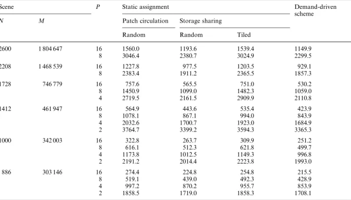
Table 1. Relative performance results in parallel execution times (in seconds) of various parallel algorithms for the form-factor computation phase
Scene P Static assignment Demand-driven
scheme
N M Patch circulation Storage sharing
Random Random Tiled
2600 1 804 647 16 1560.0 1193.6 1539.4 1149.9 8 3046.4 2380.7 3024.9 2299.5 2208 1 468 539 16 1227.8 977.5 1203.5 929.1 8 2383.4 1911.2 2365.5 1857.3 1728 746 779 16 757.6 565.5 751.0 530.2 8 1450.9 1099.0 1482.3 1059.0 4 2719.5 2161.5 2909.9 2110.8 1412 461 947 16 564.9 443.6 535.4 423.9 8 1078.1 867.1 994.0 843.9 4 2032.6 1700.7 1923.0 1684.9 2 3764.7 3399.2 3594.3 3365.3 1000 342 003 16 322.8 263.7 309.9 251.2 8 616.1 512.3 621.8 499.7 4 1173.8 1012.5 1149.3 996.8 2 2191.2 2014.4 2223.8 1993.0 886 303 146 16 274.4 224.8 254.8 215.5 8 519.1 439.0 492.3 428.9 4 997.2 870.2 955.7 853.9 2 1858.5 1719.0 1858.3 1708.1
into the global inner product operation at step 2a-b in Fig. 5.
8 Experimental results
The algorithms discussed in this work were imple-mented (in the C language) on a 4D Intel iPSC/2 hypercube multicomputer. These algorithms were tested on various room scenes containing various objects discretized into varying numbers of patches ranging from 496 to 2600.
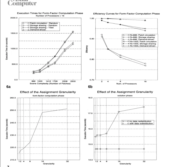
Table 1 illustrates the relative performance results of various parallel algorithms for the form-factor computation phase. The execution times of the algorithms are illustrated in Fig. 6a for 16 proces-sors. Parallel timing results for the random as-signment scheme denote the average of 5 different executions for different random assignments. As is seen in the table, the storage sharing scheme gives better performance results than the patch circula-tion scheme. In the storage sharing scheme, ran-dom decomposition yields a better load balance than the tiled decomposition, as is expected.
How-ever, tiled assignment in the storage sharing scheme yields better results in most of the test instances (e.g., 15 out of 19) than the random assignment in patch circulation due to the de-crease in communication overhead. As seen in Table 1 and in Fig. 6a, the demand-driven scheme always performs better than the static assignment scheme due to a better load balance. Note that experimental timing results for some of the instan-ces are missing for a small number of proinstan-cessors due to insufficient local memory sizes. The se-quential timings could only be obtained for the smallest scenes with N"886 and N"1000 as 3418.7 s and 3981.3 s, respectively. The efficiency curves for these scenes are illustrated in Fig. 6b. The demand-driven scheme yields almost 0.99 ef-ficiency even for these two small scenes on a hy-percube with 16 processors.
We have also experimented on the effect of the
assignment granularity on the form-factor
compu-tation and solution phases for the demand-driven assignment scheme. The results of these experi-ments are displayed in Fig. 7. The assignment granularity denotes the number of patches
6a
7
6b
Fig. 6a, b. Form-factor computation phase: a execution times for various schemes on 16 processors; b efficiency curves for various schemes
Fig. 7. The effect of the assignment granularity on the performance (execution time in seconds) of the demand-driven scheme for N"886, P"16
assigned and sent to the requesting idle processor by the host processor. A small assignment granularity (e.g., single patch assignment) gives better performance in the parallel form-factor computation phase due to the better load balance in spite of the increased communication overhead. Therefore, we can deduce that the calculation of a single form-factor row is computationally
inten-sive, and hence the load balance is a more crucial factor than the communication overhead in this scheme. As is also seen in the figure, a similar behavior is observed in the solution phase when nonzero entries are not redistributed. Note that higher granularity means a processor will gener-ate more rows for a single request. Hence, the number of nonzero entries in the local slices of the
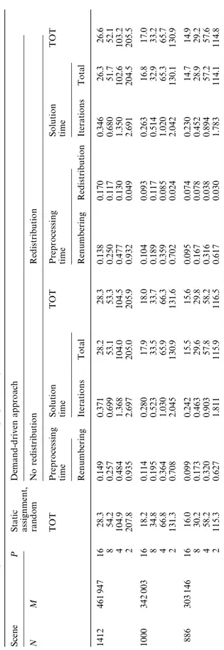
Tabl e 2 . Par a ll el exe cu ti o n ti m es (i n seco nd s) o f vari o us sc h eme s in th e so lu ti o n ph as e (u si n g th e GJ met h o d ) a lo n g w it h th e a sso ci a te d o verh eads. T h e to tal execu ti o n ti m e (T OT) inc lu di ng ov er h ea d s, i. e. , T O T " (s ol ut io n # prep ro cessi ng) ti m e S cen e P S tat ic De man d -d ri v en a p p ro a ch a ss ig n me nt , NM ran d o m N o red ist ri b u ti o n Re d is trib u ti o n TO T P re pr oce ss in g So lu ti on TO T P re pr oce ss ing So lu ti on TO T ti m e ti m e ti m e ti m e R enu m b er ing It er a ti o ns T o ta l R enu m b er ing R edi st ri b u ti o n It er a ti o ns T o ta l 1412 461 9 4 7 1 6 28. 3 0 .149 0. 371 28. 2 28. 3 0 .138 0. 170 0. 346 26. 3 26. 6 8 54. 2 0 .257 0. 699 53. 1 53. 3 0 .250 0. 117 0. 680 51. 7 52. 1 4 104. 9 0 .484 1. 368 104. 0 104. 5 0 .477 0. 130 1. 350 102. 6 103. 2 2 207. 8 0 .935 2. 697 205. 0 205. 9 0 .932 0. 049 2. 691 204. 5 205. 5 1000 342 0 0 3 1 6 18. 2 0 .114 0. 280 17. 9 18. 0 0 .104 0. 093 0. 263 16. 8 17. 0 8 34. 8 0 .195 0. 523 33. 5 33. 7 0 .189 0. 117 0. 514 32. 9 33. 2 4 66. 8 0 .364 1. 030 65. 9 66. 3 0 .359 0. 085 1. 020 65. 3 65. 7 2 131. 3 0 .708 2. 045 130. 9 131. 6 0 .702 0. 024 2. 042 130. 1 130. 9 886 303 1 4 6 1 6 16. 0 0 .099 0. 242 15. 5 15. 6 0 .095 0. 074 0. 230 14. 7 14. 9 8 30. 2 0 .173 0. 463 29. 6 29. 8 0 .167 0. 078 0. 452 28. 9 29. 2 4 58. 2 0 .320 0. 903 57. 8 58. 2 0 .316 0. 038 0. 894 57. 2 57. 6 2 115. 3 0 .627 1. 811 115. 9 116. 5 0 .617 0. 030 1. 783 114. 1 114. 8
F matrix in each processor may be substantially different, incurring more load imbalance in the solution phase for higher granularity values. As is expected, when the data are redistributed, the execution time of the solution phase remains con-stant, irrespective of the assignment granularity. Table 2 illustrates the performance comparison of various schemes in the solution phase along with the associated overheads. Note that static assign-ment scheme does not necessitate any renumber-ing operation. As is expected, data redistribution achieves performance improvement due to better load balancing in spite of the preprocessing over-heads. The overall performance gain will be much more notable for repeated solution operations as are required in lighting simulations, since the data are redistributed only once for such applications. As is seen in this table, the time spent for the renumbering and data redistribution operation is substantially smaller than even the solution time per iteration and yields a considerable improve-ment in performance during the parallel solution. For example, by spending almost 0.6% of the solution time in data redistribution, we reduce the total solution time by almost 7.1% on 16 proces-sors for the scene with N"1412 patches. The relative performance gain achieved by adopting data redistribution is expected to increase with an increasing number of processors. Table 2 also illustrates the decrease in the execution time of the parallel renumbering operation whenever the data redistribution operation is performed. This is due to the fact that the load balance metric in both the parallel renumbering and the matrix vector product operations are exactly the same; i.e., there are equal numbers of nonzero matrix elements in each processor.
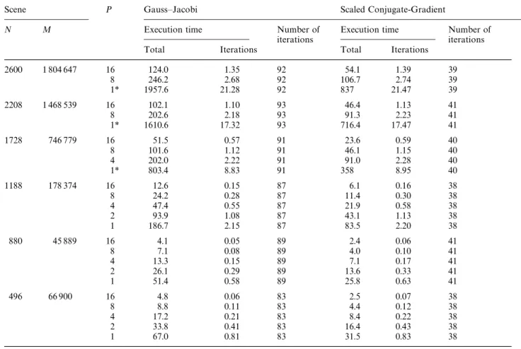
Table 3 illustrates the performance comparison of the GJ and SCG methods for the parallel solution phase. Note that experimental timing results for some of the instances on a small number of pro-cessors are missing due to the insufficient local memory size. However, sequential timings for the scenes with N"1728, 2208, and 2600 patches are estimated with the sequential complexity expres-sions given in Eqs. 4 and 8 and with tcalc"5.87 ks for the sake of efficiency computations. The number of iterations denote the total number of iterations required for convergence to the same
tolerance value (5]10~6) for three color bands
Table 3. Performance comparison of parallel the Gauss—Jacobi (GJ) and Scaled Conjugate-Gradient (SCG) methods (1* denotes the estimated sequential timings)
Scene P Gauss—Jacobi Scaled Conjugate-Gradient
N M Execution time Number of Execution time Number of
iterations iterations
Total Iterations Total Iterations
2600 1 804 647 16 124.0 1.35 92 54.1 1.39 39 8 246.2 2.68 92 106.7 2.74 39 1* 1957.6 21.28 92 837 21.47 39 2208 1 468 539 16 102.1 1.10 93 46.4 1.13 41 8 202.6 2.18 93 91.3 2.23 41 1* 1610.6 17.32 93 716.4 17.47 41 1728 746 779 16 51.5 0.57 91 23.6 0.59 40 8 101.6 1.12 91 46.1 1.15 40 4 202.0 2.22 91 91.0 2.28 40 1* 803.4 8.83 91 358 8.95 40 1188 178 374 16 12.6 0.15 87 6.1 0.16 38 8 24.2 0.28 87 11.4 0.30 38 4 47.4 0.55 87 21.9 0.58 38 2 93.9 1.08 87 43.1 1.13 38 1 186.7 2.15 87 83.5 2.20 38 880 45 889 16 4.1 0.05 89 2.4 0.06 41 8 7.1 0.08 89 4.0 0.10 41 4 13.3 0.15 89 7.1 0.17 41 2 26.1 0.29 89 13.6 0.33 41 1 51.4 0.58 89 25.8 0.63 41 496 66 900 16 4.8 0.06 83 2.5 0.07 38 8 8.8 0.11 83 4.4 0.12 38 4 17.2 0.21 83 8.4 0.22 38 2 33.8 0.41 83 16.4 0.43 38 1 67.0 0.81 83 31.5 0.83 38
Fig. 8. Efficiency curves for the SCG method
individual SCG iteration takes more time than that of the GJ iteration. However, the SCG method converges much faster than the GJ method, as is expected. Therefore, we recommend the parallel SCG method for the solution phase. Figure 8 illustrates the efficiency curves of the SCG method. As is seen in this figure, the efficien-cy remains above 86% for sufficient granularity (i.e., M/P'11 148).
9 Conclusions
In this work, a parallel implementation of the gathering method for hypercube-connected multi-computers has been discussed for applications in which the location of objects and light sources remain fixed, whereas the intensity and color of the light sources and/or reflectivity of objects vary
in time, such as in lighting simulations. In such applications, the efficient parallelization of the solution phase is important since this phase is repeated many times.
The powerful scaled conjugate-gradient (SCG) method has been successfully applied in the solu-tion phase. It has been shown that the non-symmetric form-factor matrix can be efficiently transformed into a symmetric and positive defi-nite matrix to be used in the SCG method. It has been experimentally observed that the SCG algo-rithm converges faster than commonly used Gauss—Jacobi (GJ) algorithm, which converges in almost double the number of iterations of the SCG algorithm. Efficient parallel SCG and GJ algorithms were proposed and implemented. An almost perfect load balance has been achieved by a new and efficient parallel data redistribution scheme. Our experiments verify that the efficiency of the SCG algorithm with the data redistribution scheme remains over 86% for sufficiently large granularity (i.e., M/P'11 148). We conclude that the SCG method is a much better alternative to the conventional GJ method for the parallel solu-tion phase.
In this paper, several parallel algorithms for the form-factor computation phase were also present-ed. It has been illustrated that it is possible to reduce the interprocessor communication by sharing the memory space for rows of the form-factor matrix with global patch data. It has also been observed that the demand-driven approach, in spite of its extra communication overhead, achieves better load balancing and hence better processor utilization than static assignment. An efficient parallel renumbering scheme has also been proposed to avoid double indexing required in the matrix vector products in the parallel SCG and GJ algorithms when demand-driven assign-ment is used in the form-factor computation phase.
Acknowledgements. This work is partially supported by the
Commission of the European Communities, Directorate General for Industry under contract ITDC 204-82166, and The Scientific and Technical Research Council of Turkey (TU®BI0 TAK) under grant EEEAG-160.
References
1. Aykanat C, O®zgu¨ner F, Erial F, Sadayappan P (1988) Iterative algorithms for solution of large sparse systems of
linear equations on hypercubes. IEEE Trans Comput 37:1554—1568
2. Aykanat C, hapin TK, O®zgu¨i B (1996) A parallel progressive radiosity algorithm based on patch data circulation. J Com-put Graph 20:307—324
3. Baum DR, Rushmeier HE, Winget JM (1989) Improving radiosity solutions through the use of analytically deter-mined form-factors. Comput Graph 23:325—334
4. Chalmers AG, Paddon DJ (1989) Implementing a radiosity method using a parallel adaptive system. Proceedings of the 1st International Conference on Applications of Trans-puters, Liverpool, UK
5. Chalmers AG, Paddon DJ (1990) Parallel radiosity methods. The 4th North American Transputer Users Group Confer-ence, Ithaca, USA, IOS Press, pp 183—193
6. Chalmers AG, Paddon DJ (1991) Parallel processing of progressive refinement radiosity methods. Proceedings of the 2nd Eurographics Workshop on Rendering, Barcelona, Spain
7. Cohen MF, Greenberg DP (1985) The hemi-cube: a radiosity solution for complex environments. Comput Graph (SIGGRAPH’85) 19:31—40
8. Cohen MF, Chen S, Wallace J, Greenberg DP (1988) A pro-gressive refinement approach for fast radiosity image generation. Comput Graph 22:75—84
9. Drucker SM, Schroeder P (1992) Fast radiosity using a data parallel architecture. Proceedings of the 3rd Euro-graphics Workshop on Rendering, Bristol, UK, pp 247—258 10. Feda M, Purgathofer W (1991) Progressive refinement radiosity on a transputer network. Proceedings of the 2nd Eurographics Workshop on Rendering, Barcelona, Spain
11. Golub GH, van Loan CF (1989) Matrix computations, 2nd edn. The Johns Hopkins University Press, Baltimore, Maryland
12. Goral CM, Torrance KE, Greenberg DP, Battaile B (1984) Modeling the interaction of light between diffuse surfaces. Comput Graph 18:213—222
13. Guitton P, Roman J, Schlick C (1991) Two parallel approaches for a progressive radiosity. Proceedings of the 2nd Eurographics Workshop on Rendering, Barcelona, Spain
14. Hestenes MR, Stiefel E (1952) Methods of conjugate gradi-ents for solving linear systems. Natl Bureau Stand J Res 49:409—436
15. Ja´ja´ J, Ryu KW (1992) Load balancing and routing on the hypercube and related networks. J Parallel Distributed Comput 14:431—435
16. Jessel JP, Paulin M, Caubet R (1991) An extended radiosity using parallel ray-traced specular transfers. Proceedings of the 2nd Eurographics Workshop on Rendering, Barcelona, Spain
17. Neumann L (1994) New efficient algorithms with posi-tive definite radiosity matrix. Proceedings of the 5th Euro-graphics Workshop on Rendering, Darmstadt, pp 219—237 18. Neumann L, Tobler R (1995) New efficient algorithms with positive definite radiosity matrix. In: G. Sakas, P. Shirley, and S. Mu¨ller (eds) Photorealistic Rendering Techniques. Springer, pp 227—243
19. Paddon D, Chalmers A, Stuttard D (1993) Multiprocessor models for the radiosity method. Proceedings of the 1st Bilkent Computer Graphics Conference on Advanced Tech-niques in Animation, Rendering, and Visualization. Ankara, Bilkent Univ., Ankara, pp 85—103
20. Price M, Truman G (1990) Radiosity in parallel. Application of transputers: Proceedings of the 1st International Confer-ence on Applications of Transputers, IOS Press, Amster-dam, pp 40—47
21. Purgathofer W, Zeiller M (1990) Fast radiosity by paralleli-zation. Proceedings of the Eurographics Workshop on Photosimulation, Realism and Physics in Computer Graphics, Rennes, pp 173—184
22. Ranka S, Sahni S (1990) Hypercube algorithms with applica-tions to image processing and pattern recognition. Bilkent University Lecture Series, Springer, Berlin Heidelberg New York
23. Ryu KW, Ja´ja´ J (1990) Efficient algorithms for list ranking and for solving graph problems on the hypercube. IEEE Trans Parallel Distributed Syst 1:83—90
24. Varshney A, Prins JF (1992) An environment-projection approach to radiosity for mesh-connected computers. Pro-ceedings of the 3rd Eurographics Workshop on Rendering, Bristol, UK, pp 271—281
25. Watt A (1989) Fundamentals of three-dimensional computer graphics. Addison Wesley, Wokingham New York Amster-dam Bonn
26. Whitman S (1992) Multiprocessor methods for computer graphics rendering. Jones and Bartlett Boston
TAHSI0 N M. KURh received his B.S. degree in Electrical and Electronics Engineering from the Middle East Technical Uni-versity, Ankara, Turkey, in 1989 and his M.S. degree in Com-puter Engineering and Informa-tion Science from Bilkent Uni-versity, Ankara, Turkey, in 1991. He is currently a Ph.D. student at Bilkent University. His re-search interests include parallel computing and algorithms, parallel computer graphics ap-plications, visualization, and rendering.
CEVDETAYKANAT received his B.S. and M.S. degrees from the Middle East Technical Uni-versity, Ankara, Turkey, and his Ph.D. degree from Ohio State University, Columbus, all in electrical engineering. He was a Fulbright Scholar during his Ph.D. studies. He worked at the Intel Supercomputer Systems Division Beaverton, as a re-search associate. Since October 1988 he has been with the De-partment of Computer Engin-eering and Information Science, Bilkent University, Ankara, Tur-key, where he is currently an associate professor. His research interests include parallel computer architectures, parallel algo-rithms, parallel computer graphics applications, neural network algorithms, and fault-tolerant computing.
BU®LENT O®ZGU®C, joined the Bilkent University Faculty of Engineering, Turkey, in 1986. He is a professor of computer science and the dean of the Fac-ulty of Art, Design and Architec-ture. He formerly taught at the University of Pennsylvania, USA, Philadelphia, College of Arts, USA, and the Middle East Technical University, Turkey, and worked as a member of the research staff at the Schlumber-ger Palo Alto Research Center, USA. For the last 15 years, he has been active in the field of computer graphics and animation. He received his B. Arch. and M. Arch. in architecture from the Middle East Technical Univer-sity in 1972 and 1973. He received his M.S. in architectural technology from Colombia University, USA, and his Ph.D. in a joint program of architecture and computer graphics from the University of Pennsylvania in 1974 and 1978, respectively. He is a member of ACM Siggraph, IEEE Computer Society and UIA.