Preferences, selection, and value added: a structural approach

a_{Bilkent University,Turkey}

b_{The Pennsylvania State University,United States}

A R T I C L E I N F O

A B S T R A C T

What do applicants take into consideration when choosing a high school? To what extent do schools contribute to their students' academic success? To answer these questions, we model students' preferences and obtain average valuation placed on each school. We then investigate what drives these valuations by carefully controlling for endogeneity using a set of creative instruments suggested by our model. Wefind that valuation is based on a school's location, its selectivity as measured by its cutoff score, value added and past performance in university entrance exams. However, cutoffs affect school valuation an order of magnitude more than does value added.

“The C student from Princeton earns more than the A student from Podunk not mainly because he has the prestige of a Princeton degree, but merely because he is abler. The golden touch is possessed not by the Ivy League College, but by its students.”

Shane Hunt, “Income Determinants for College Graduates and the Return to Educational Investment,” Ph.D. thesis, Yale University, 1963, p. 56.

1. Introduction

In much of the world, elite schools are established and very often subsidized by the government. Entry into these“exam” schools is based on performance in open competitive entrance exams. Applicants leave no stone unturned in their quest for higher scores on these entrance exams, creating enormous stress. The belief seems to be that getting into these schools is valuable, presumably because future outcomes are better in this event. Students, it is argued, will do better by going to an exam school where they are challenged by more difficult material and exposed to better peers. What actually happens? Students of these elite exam high schools, without a doubt, do better on college entrance exams and are more likely to be placed at the best university programs. But is this due to selection or value-added by these schools? It is quite possible that the success of students from exam schools creates the belief that these schools add value. This belief results in better students sorting into exam schools so that students from these schools do better, which perpetuates the belief system.

The usual way of ranking schools is in terms of their selectivity, how hard they are to get into in terms of some performance measure like the SATs in the US,1_{or in terms of how well students who graduate from them do as measured by wages, eminence in}

http://dx.doi.org/10.1016/j.euroecorev.2016.09.009 Received 22 September 2015; Accepted 15 September 2016

⁎_{Corresponding author.}

E-mail addresses:pelina@bilkent.edu.tr(P. Akyol),kmk4@psu.edu(K. Krishna).

1_{Schools are sometimes less than honest: some inflate their statistics on the performance of their entering class. Some schools manipulate the system by keeping}

their class size small, thereby having high SATs and looking very selective. See“Academic integrity should count in rankings” in the Kansas City Star, 2/8/2013. http://www.centredaily.com/2013/02/12/3499088/editorial-academic-integrity-should.html

Available online 28 September 2016

later life, or admission into further schooling. However, schools may do well in all of these dimensions merely because they admit good students and not because they provide value added and thereby improve the performance of the students they admit.2_{How can}

we control for such selection and estimate value added? What do students seem to value? Can we model and estimate their preferences? These are the questions we try to address.

Turkey is a good place to look for answers to these questions for a number of reasons. To begin with, the Turkish admissions system is exam-driven. Admissions are rationed on the basis of performance on open competitive national central exams at the high school and university level. This eliminates incentive problems when there are a large number of students.3Second, as education is highly subsidized in public institutions, educational options outside the country or at private institutions are much more expensive so that these exams are taken seriously by the applicants. When the stakes are high, as in Turkey, it is less likely that outcomes are driven just by noise.

We develop a way to answer the questions of interest by taking a more structural approach than much of the literature. The structure imposed allows us to economize on the data requirements. Our data consists of information on all high schools (Exam Schools) in Turkey which admit students on the basis of an open competitive exam administered at the end of middle school. Not all middle schoolers take this exam as it is voluntary. We obtained (from public sources) the admission cutoff scores of each exam school, the number of seats in each such school, and the overall distribution of scores of students who chose to take this exam. For one school only, we also have the distribution of scores of admitted students. We also have the mean performance of students in each exam high school in the university entrance exam. We would like to emphasize that we do not have individual level data on performance in the high school (or university entrance) exam or on stated preferences for high schools.

We use this data inSection 3to estimate a nested logit model of preferences over high schools, taking into account that exam schools only admit the highest scoring students who apply. Thus, students choose their best school from schools whose cutoff is below their score. We estimate preferences in two steps. First, by using information on the minimum cutoff scores, we derive the demand for each school, conditional on the correlation of shocks within a nest. We obtain the mean valuation for each school by setting demand equal to the number of available seats and solving for mean valuation. Second, we pin down the correlation of shocks within a nest using information on the maximum and minimum cutoff scores in each school. This twist, to our knowledge, is novel. The idea is quite simple. If preference shocks are perfectly correlated within a nest, then preferences are purely vertical and the minimum score in the most valued school in the nest cannot be lower than the maximum score in the second most valued school in the nest. Thus, the extent of overlap in the scores between schools within a nest identifies the correlation in preference shocks in the nest.

Finally, inSection 3, to see what applicants care about in a school, we regress the mean valuation of schools on the schools' characteristics (its location, size, mean performance in the verbal and quantitative parts of the university entrance exam, type of school, and the cutoff score). The error term, which is meant to capture shocks to school valuations, is likely to be correlated with the cutoff, as greater valuations raise demand and hence the cutoff, biasing the estimates upwards. We use a clever instrument suggested by our model to correct for endogeneity bias. Wefind that selectivity does indeed seem to raise valuations.

Section 4focuses on value added. In this section we restrict attention to a subset of schools (Science high schools). To understand the value added by a school, we use the data on the overall distribution of scores on the high school entrance exam, along with the estimated preference parameters, to allocate students to high schools and obtain the simulated distribution of students' scores on the high school entrance exam in each school. We then compare the mean of the simulated distribution for each school to its mean score in the University Entrance Exam after standardizing the scores. This gives a (possibly contaminated by mean reversion) estimate of the value-added by a school. Mean reversion is likely to be especially severe at the top and bottom of the school hierarchy as it is a consequence of randomness in performance. Students in the best (worst) schools disproportionately include those who are just lucky (unlucky) so that their performance in the university entrance exams will tend to be below (above) that in the high school entrance exams even if there is zero value added. We use simulation-based methods as well as information on each student in a single school to estimate the average value-added by a school, while controlling for mean reversion. Note that the extent of the mean reversion depends on both preferences and the extent of noise in the high school entrance exam score so that correcting for it can only be done by taking a structural approach. Finally, we ask if value added also drives mean valuation of a school.

Our results show that highly valued schools do not all have high value-added. Some have negative value added, while others have positive value added. Our estimates suggest that students like more selective schools so that better students, who have more options open to them, sort into these schools. We alsofind that they also care about the value added by the school, but its importance (in a standardized regression) is far less than that of the cutoff score. Consequently, even when schools do not add value to the students (in terms of their performance on the university entrance exam) they attract good students, providing an advantage to incumbents and an impediment to entry and the functioning of the market.

A major contribution of our paper is to relate the valuations placed on schools to measures of school characteristics such as selectivity, facilities, location and value added by the school. It is important to understand what lies behind preferences. If preferences seem to be driven by selectivity alone, selective schools need not be those that are adding the most value and circular causation will drive rankings. Preferences may be unrelated to school performance (i.e., value added) either because it is hard to

2_{There has recently been considerable effort in determining value-added by a school as part of the accountability in the No Child Left Behind legislation. See}

Darling-Hammond et al. (2012)for a critique of the approach usually taken.

countries. While the evidence on the effect of attending more selective schools on students' academic achievement is mixed, one possible interpretation is that just attending a more selective school is not enough to improve future performance. An essential input might also be the motivation of students. This could be manifested in the data as they are choosing to attend a more selective school, despite it being harder in some dimension for them to do so.

In the US, the consensus seems to be that expanding school options, via having exam schools or having lotteries that allow the winners more school options, need not have much of an impact on a student's academic achievement.Abdulkadiroğlu et al. (2014) andDobbie and Fryer Jr (2011) find going to exam schools has little effect on academic achievements using a Regression-Discontinuity approach in Boston and New York, respectively.Cullen et al. (2005, 2006)use data from randomized lotteries that determine the allocation of students in the Chicago public school system. Students who win the lottery have more options open to them and so can attend schools more consistent with their tastes and hence are better off.5

Theyfind that winning this lottery does not improve students' academic performance. In contrast to work thatfinds little effect of expanding school options,Hastings et al. (2012)use U.S. data from a low income urban school district andfind that winning this lottery has a positive and significant effect on both student attendance after winning the lottery but before going to the new school, and on performance later on.Clark (2010) investigates the effect of attending a selective high school (Grammar School) in the UK (where selection is based on a test given at age 11 and primary school merit) andfinds no significant effect on performance in courses taken by students, although the probability of attending a university is positively affected.

Dale and Krueger (2002, 2011)look at the effect of attending elite colleges on labor market outcomes. They control for selection by controlling for the colleges to which the student applied and was accepted. The former provides an indication of how the student sees himself, while the latter provides a way of controlling for how the colleges rank the student. Intuitively, the effect of selective schools on outcomes is identified by the performance of students who go to a less selective school despite being admitted to a more selective one, relative to those who go to the more selective one. Of course, if this choice is based on unobservables, this estimate would be biased.6_{Theyfind that black and Hispanic students as well as students from disadvantaged backgrounds (less-educated or}

low-income families) do seem to gain from attending elite colleges. However, for most students the effect is small and fades over time.

Duflo et al. (2011)emphasize an important additional channel that may induce heterogeneity in effects. If, for example, teachers at a top ranked school direct instruction towards the top, ignoring weaker students, better students in the class may gain, while worse ones may lose. In such cases the value added of a school can vary by student ability and tracking may help teachers target students.

Card and Giuliano (2014)look at the effect of being in gifted programs. They find that high IQ students, to whom these programs are often targeted, do not seem to gain from such programs. However, students who miss the IQ thresholds but scored highest among their school/grade cohort in state-wide achievement tests in the previous year do gain. Their work suggests that“a separate classroom environment is more effective for students selected on past achievement – particularly disadvantaged students who are often excluded from gifted and talented programs.”

In contrast to these results,Pop-Eleches and Urquiola (2013)andKirabo Jackson (2010)estimate the effect of elite school attendance in Romania and Trinidad and Tobago, respectively. Theyfind a large positive effect on students' exam performance in the university entrance exams. This could be because students who go to elite schools in these countries are more motivated to succeed than those going to elite schools in richer countries.

From the school choice literature,Hastings et al. (2008)andBurgess et al. (2009)investigate what parents care about in a school using data from the Charlotte-Mecklenburg School District and Millennium Cohort Study (UK), respectively.Hastings et al. (2008) take a structural approach and estimate a mixed logit model of preferences. A major contribution of their work is to use information on the stated preferences for schools and compare these to what was available to them to back out the weight placed on factors like academics, distance from home, and so on. They are then able to see whether the impact of a school differs according to “type”. They

4_{This regressive nature is common across countries as the better off are advantaged in many ways.}

5_{The schools they choose may be those that add value through delivering higher achievement levels, better peers and more resources, or not.}

6_{For example, if confident students go to the selective school and less confident ones do not, and confident students do better, the effect of selective schools would}

find that students who put a high value on academics in so much as they choose to go to “supposedly good” schools that are further away, do better from being there than students who attend just because they are close to the school. For this reason, reduced form effects estimated for attending “good” schools could be biased when such selection is not properly accounted for. If students in developing countries place greater value on good schools than do students from developed countries, this insight could explain why we see such different results for attending better schools in the two.Burgess et al. (2009)also compare thefirst choice school, to the set that was available (constructed by the authors by using students' residence areas) and estimate trade-offs between school characteristics.

An advantage of the slightly more structural approach taken here is that we examine the whole process and not just one of its components in the estimation. Our approach allows us to separate between preferences over schools (based on their observable attributes) and their value added. Moreover, despite the lack of panel data, i.e., not having the high school entrance exam score and the college entrance exam score for each student, we show how one can use fairly limited data on each high school, along with data on university entrance exam takers along with the model, to get around this deficiency. That is to say, our approach allows us to economize on data in the estimation which extends the ability to look at policy issues, as outcomes may differ across countries. Of course, the applicability of our method depends on certain institutional characteristics, such as priority by score in the allocation of students to high schools, and the existence of uniform school leaving or university entrance exams. While our approach has many limitations, for example, it does not allow us to look at whether attending elite exam schools has heterogeneous effects, nor does it let us look at long term effects (which may be large even if short term ones are not7) as inChetty et al. (2014a), it does provide a way to do a lot with relatively little data.

2. Background

In Turkey, competitive exams are everywhere. Unless a student chooses to attend a regular public high school, he must take a centralized exam at the end of 8th grade to get into an“exam school”. These are analogous to magnet schools in the US, though the competition for placement into them is national and widespread, rather than local as in the US. After high school there is an open competitive university entrance exam given every year. Most students go to cram schools (dershanes) to prepare for the university entrance exam. Much of high school is also spent preparing students for this exam. In fact, it has been argued that at least in Turkey, cram schools weaken the formal schooling system as students substitute cram schools (dershanes) for high school (seeTansel and Bircan, 2006). If exam schools, in fact, have little value-added, then the system itself may have adverse welfare effects. This is especially so if these elite exam schools are subsidized relative to the alternatives as is often the case.8_{In this event, students expend}

possibly wasteful effort to capture these rents which has a welfare cost.9

Students from exam schools do perform much better in university entrance exams.Fig. 1shows the distribution of average scores (ÖSS-SAY) in the university entrance exam of science track students coming from the different kinds of high schools. Science high schools are clearly doing better, followed by the almost equally selective Anatolian high schools, while regular public schools seem to do the worst. However, this says little about the contribution of exam schools in terms of value-added.

2.1. The institutional structure

The educational system in Turkey is regulated by the Ministry of Education. All children between the ages of 6 and 14 must go to school. At 14 they take the high school entrance exam (OKS) if they want to be placed in public exam schools. Performance on this exam determines the options open to a student. The better the performance, the greater the number of schools with a cutoff score below what the student has obtained. There are four types of public exam schools: Anatolian high schools, Anatolian Teacher Training high schools, Science high schools, and Anatolian Vocational high schools.

Anatolian high schools place a strong emphasis on foreign language education although their specific goals may vary across the different types of Anatolian schools. The main goal of Anatolian high schools is to prepare their students for higher education while teaching them a foreign language at a level that allows them to follow scientific and technological developments in the world. Anatolian Vocational high schools aim to equip their students with skills for certain professions and prepare them both for the labor market and higher education. Anatolian Teacher Training high schools train their students to become teachers though they can choose other paths as well.

The most prestigious of the exam schools are the Science high schools. These were established in the mid-1980s to educate the future scientists of Turkey and initially accepted very few students. Over the next decade, the success of their students on the university entrance exams, as well as the rigorous education these schools were famous for, created considerable demand for these schools and they spread throughout the country.

In public high schools, students can choose between four tracks: the Science track, the Turkish-Math track, the Social Science track and the Language track. They make this choice after ninth grade. In Science high schools they must take the science track. In Anatolian Vocational high schools there are no tracks, which put them a little outside the mainstream. All of this is depicted inFig. 2. After eleventh grade, students who wish to pursue higher education take a centralized nationwide university entrance exam (ÖSS), which is conducted by the Student Selection and Placement Center (ÖSYM). There are no selection issues here: data (from the

7_{Zimmerman (2014)suggests that elite school attendance may have long term impacts via networks and referrals.}

8_{The best teachers are allocated to these schools, their facilities are better, and their class sizes are smaller than that of regular schools. In addition,Caner and}

Okten (2013)show that school subsidies are regressive as better off students tend to do better on exams and so go to better schools which are more highly subsidized.

National Education Statistics Bureau) on the number of high school graduates and data on the number of students taking the university entrance exam for thefirst time (from reports released by ÖSYM) show that these two are very close to each other. This exam is highly competitive and placement of students into colleges is based on their ÖSS score, high school grade point average (GPA), and their preferences.

Below, we use high school and university entrance exam scores to infer the value-added of schools. For this reason, it is important to explain what these exams consist of and how similar they are. Both high school and university entrance exams are multiple choice tests that are held once a year. The high school entrance exam is taken by students at the end of eighth grade. There are four tests, Turkish, social science, math, and science, with 25 questions on each test. Students are given 120 min to answer the 100 questions. The University entrance exam is similar. It is a nationwide central exam with four parts, Turkish, social science, math, and science,

Fig. 1. Distribution of ÖSS-SAY score.

with 45 questions in each part. Students are given 180 min. The questions on both exams are based on the school curriculum and are meant to measure the ability to use the concepts taught in school. To discourage guessing, there is negative marking for incorrect answers in both exams.

2.2. The data

The data we use come from several public sources. To measure students' academic performance at the end of high school, we rely on information on the performance of each school on the university entrance exam from 2002 to 2007. This information is published by ÖSYM and is made available to schools and families so that they are informed about the standing of each school. The information includes the number of students who took university entrance exam from each school, as well as the mean and standard deviation of their scores in eachfield of the exam.

A student's performance in the high school entrance exam is seen as a (noisy) measure of his performance prior to attending high school. We obtained data on the minimum and maximum admission scores and on the number of seats in 2001 for each exam high school from the Ministry of Education's website.10_{The summary statistics for these variables are presented inTable A6. We also}

collected data on the average ÖSS performance of each high school on each part of the exam in the previous year, 2000, from ÖSYM's Results booklet for that year, which is publicly available from their website. This is used as one possible quality dimension along which schools vary. Additional high school characteristics were collected from the Ministry of Education's website (education language, dormitory availability, and location) and the high schools' websites (age of the schools). We use this data along with the score distribution of all students who took the high school entrance exam in 2005 (seeTable A7) in our analysis below. Ideally we would have liked to have this information for 2001, but as this was not available and as these distributions are very stable, we use data from 2005.

In the next section we show how to use information on the allocation process, seats available, the distribution of scores overall on the high school entrance exam, and the preference structure to back out the mean valuation placed on each high school.

3. The model

Seats in public exam schools are allocated according to students' preferences and their performance on a centralized exam (conducted once a year). All schools have an identical ranking over students based on their test scores. Each exam school has afixed quota, qj, which is exogenously determined.11The allocation process basically assigns students to schools according to their stated

preferences, with higher scoring students placed before lower scoring ones. Students know past cutoffs for schools when they put down their preferences. They are allowed to put down up to 12 schools.12

We model preferences as follows. Student i's utility from attending school j takes the form U X ξ εij( ,j j, ij; ) =β βXj+ξj+εij

where Xjare the observed school characteristics,ξjare the unobserved school characteristics, andεijis a random variable which has

a Generalized Extreme Value (GEV) distribution. Letδjdenote the school specific mean valuation where

δj=βXj+ξj

so that

U X ξ εij( ,j j, ij; ) =β δj+εij

This structure implies that variation in individual preferences comes from the error term, conditional on the students having the same feasible choice set.13_{Preference shocks are allowed to be correlated for the alternatives in the same nest. Otherwise, they are}

assumed to be independent.

In general, the cumulative distribution function of ε= 〈εi0,εi1, …,εiN〉is given by ⎛ ⎝ ⎜ ⎜ ⎛ ⎝ ⎜ ⎜ ⎛_⎝⎜ ⎞_⎠⎟ ⎞ ⎠ ⎟ ⎟ ⎞ ⎠ ⎟ ⎟

∑ ∑

10_{This data was collected using the websitehttp://archive.org/web/web.php, which provides previous versions of websites.} 11_{In general, the seats available are close to the size of the graduating class as schools are capacity constrained.}

12_{Students do face a location restriction in listing their Anatolian high school preferences. They are not allowed to list preferences on Anatolian high schools in}

Ankara,İstanbul, İzmir, and their current city: they have to pick one of these locations and make all their Anatolian high school preferences from their chosen location. However, if preferences are stated after the score is known, and cutoffs are stable over time (as in our setting) this restriction should not have any impact. A student would put his most preferred school with a cutoff below his score at the top of his list and be assigned there.

13_{In our model, we do not incorporate heterogeneity in valuations depending on students' score or other background characteristics as we do not have information}

on individual student's preferences. However, the choice set for each student depends on his score so that individuals with different scores make very different choices. With better data on students' scores, background characteristics, stated preferences and high school placement, we could allow valuations to depend on individual characteristics. Moreover, with such data we could do a much better job estimating school value-added and even allow for possible heterogeneous treatment effects.

alternatives within nest k (seeTrain, 2009). Asλkincreases, the correlation between alternatives in nest k decreases. Ifλkis equal to

1, there is no correlation between alternatives within nest k, whereas as λk goes to0, there is perfect correlation among all

alternatives in the same nest. In this case, the choice of alternatives for any individual is driven by theδjcomponent alone so that

there is pure vertical differentiation among schools in a nest.

We partition the set of high schools in Turkey according to their type and location.Fig. 3shows the nesting structure we adopt. Since we want to allow for vertical and horizontal differentiation, it makes sense to put similar schools in the same nest. Thus, at the upper level of the nest, students have seven options: Science high schools, Anatolian Teacher Training high schools, Anatolian high schools in Ankara, inİstanbul and in İzmir, Anatolian Vocational high schools, and the local school option. The local school option for a student includes a local Anatolian school and a public regular high school which is modeled as the outside option. Since computational intensity will increase with the size of the choice set, we aggregate Anatolian Vocational high schools intofive subgroups according to their types with seats equal to the sum of seats of schools in that subgroup. We define the maximum and minimum score of each subgroup as the maximum and minimum of the cutoff scores of the schools in that subgroup. Other nests include all schools in Turkey of a given type: 91 Teacher Training high schools, 48 Science high schools, 24 Anatolian high schools in Ankara, 38 Anatolian high schools inİ stanbul, and 18 Anatolian high schools in İzmir.14_{Thus, we have 226 options overall.}15

Each student chooses a school that maximizes his utility given his feasible set of schools, which is determined by his own score,si,

and the cutoff scores of each school U X ξ ε β max ( , , ; ) j∈-i ij j j ij where j c s = { : ≤ } i j i

-The feasible set of a student,- includes all the schools whose cutoi, ff score is below the student's score. Given the demand for each school and the number of seats available, the cutoff score, c ,j is endogenously determined in equilibrium.

Let the set of N schools be partitioned into K mutually exclusive sets (nests) where the elements of each of these sets correspond to schools within that nest. For example, Bk, where k= 1, 2, …,K, would have all schools that are in nest k as its elements. If there

were no rationing, the probability that school j in nest k was chosen by student i would be given by16

⎛ ⎝ ⎜ ⎞ ⎠ ⎟⎛ ⎝ ⎜ ⎛ ⎝ ⎜ ⎞ ⎠ ⎟⎞ ⎠ ⎟ ⎛ ⎝ ⎜ ⎛ ⎝ ⎜ ⎞ ⎠ ⎟⎞ ⎠ ⎟ δ λ P δ λ δ λ δ λ ( , ) = exp ∑ exp ∑ ∑ exp ij j k l B l k λ n K l B l n λ ∈ −1 =1 ∈ k k n n

which would be equivalent to the fraction of students whose best alternative was alternativej.

However, students' choices are constrained by the cutoff scores in each school, cj, and by their own exam performance, si.

Suppose that there areN + 1choices (including the outside option) and let the cutoff scores for each alternative be ordered in ascending order:

c0= 0 c1 c2 ⋯ cN−1 cN

Fig. 3. School choice in Turkey.

14_{These schools are located in the center of the Ankara,İstanbul, and İzmir. Anatolian high schools located in a town in the provinces are defined as local}

Anatolian high schools by Ministry of Education.

15_{We ignore private exam high schools as they comprise less than 5% of the total and there is no data on them.} 16_{SeeTrain (2009, Chapter 4)for the derivation of P .}

where 0 indexes the outside option. Students whose score is in the interval[cm,cm+1)have thefirst m schools in their feasible choice set and we call this interval Im. Similarly, students whose scores are below c1have scores in I0and have their choice set containing

only the outside option, while students with si≥cNget to choose from all theN + 1alternatives and have scores in IN. Thus, the

probability that student i with a score in Ijchooses schoolt,t≤j, in nest k from his feasible set will be

⎧ ⎨ ⎪ ⎪ ⎩ ⎪ ⎪ ⎛ ⎝ ⎜ ⎞_⎠⎟⎛ ⎝ ⎜ ⎛ ⎝ ⎜ ⎞_⎠⎟⎞ ⎠ ⎟ ⎛ ⎝ ⎜ ⎛_⎝⎜ ⎞_⎠⎟⎞ ⎠ ⎟ ⎫ ⎬ ⎪ ⎪ ⎭ ⎪ ⎪ δ λ P δ λ δ λ δ λ s I ( , ) = exp ∑ exp ∑ ∑ exp if ∈ jt k t k l B I l k λ n K l B I l n λ i j ( ) ∈ ( ) −1 =1 ∈ ( ) k j k j n j n

where bold variables denote vectors and whereB Ik( )j denotes the restriction placed on the elements of nest k when the individuals'

score is in the intervalIj. λkis the extent of independence between alternatives in nest k, and Kjis the total number of nests available

to a student whose score is in the interval Ij.

Aggregate demand for each school will thus depend on the distribution of scores,F s( ), the minimum entry cutoff scores of all other schools whose cutoff score is higher, and the observed and unobserved characteristics of all schools. Using the equilibrium cutoff scores and the students' score distribution we can get the density of students that are eligible for admission to each school. For simplicity, we will write the demand function for school j in nest s,dj s( )( , )δ λ, asdj s( ). The demand for school N , the best

school, which is in nest k comes only from those inIN:

δ λ

dN k( )=PNN k( )( , )[1 −F c(N)]

Only students with scores above cNhave the option to be in school N which gives the term[1 −F c(N)]. In addition, N in nest k has

to be their most preferred school; hence the termPNN k( )( , )δ λ. Similarly, the demand for school j which is in nest s comes from those

inIj,… IN:

∑

Students with higher scores have more options open to them which is what makes higher scores valuable to a student in this setting.

3.1. Estimation strategy and results

Given the preference parameters and the number of seats in each school, the real world cutoffs are determined by setting the demand for seats, as explained above, equal to their supply and obtaining the market clearing score cutoffs. This is not what we will do. For us, the cutoffs and the number of seats are data. We want to use this data and the nesting structure imposed to obtain the preference parameters. In particular, we want to estimate the coefficients of school characteristics( )β and the parameter vector λ, where λ= [ ,λ λ1 2, …,λK], that bestfit the data and respect the solution of the model that equates demand d( )with supply q( ).

We do this in two steps. In Step 1, we back out the values ofδjfor each school j for a given λ. In essence, the minimum cutoff in

each school denoted by the vectorc= ( , ‥c1 cN), the number of seats in each school denoted by the vectorq= ( , ‥q1 qN), together with

the market clearing conditions of the model, pin down the mean valuation of each school for a given vector, λ= ( , …λ1 λK). In step 2, wefind λ so as to best match the extent of overlap in the scores of schools in the same nest. A higher correlation in the errors within a nest means that there is less of a role for preference shocks to play in choice, so that preferences are driven by the non-random terms. This corresponds to having more of a vertical preference structure. As a result there is less overlap in the range of student scores across schools in a nest. If there is perfect correlation, the maximum score in a worse school will be less than the minimum score in a better one. Following this, we relate our estimates ofδjto the characteristics of each school to see what drives the preferences for

schools.

We do not use the standard nested logit setup because the cutoff score constrains choice. Only those students with scores above the cutoff for a school have the option of attending it. Had we ignored this constraint, we would have obtained biased estimates of δj.

For example, small and selective colleges would be wrongly seen as undesirable.17

3.2. Step 1: mean valuations conditional on λ

Our model includes unobserved school characteristics, and these unobserved characteristics enter the demand function nonlinearly, which complicates the estimation process.Berry (1994)proposed a method to transform the demand functions so that unobserved school characteristics appear as schoolfixed effects. By normalizing the value of the outside option to zero, δ = 00 , we have N demand equations with N unknowns. This permits us to get the vector δ( , , ) for given vectors q andq c λ c,conditional on a

17_{There is a growing literature on the structural estimation of matching models that uses data on who is matched with whom (seeFox, 2009). Since we do not}

vector λ such that

δ λ λ

q= ( ( , , ), ).d q c

On the left-hand side we have supply of seats, and on the right-hand side we have the demand for seats for a given vector of mean school valuations and school cutoffs (denoted by δ andc, respectively) and correlation of shocks within nests (λ). For a given λ, and with q andccoming from the data, we can invert the above to obtain δ( , , ). We cannot solve forq c λ δ q c λ( , , )analytically as done in some of the models inBerry (1994). Our setup is closer to that inBresnahan et al. (1997)who solve the system numerically as we do. Berry (1994)shows that if the market share function is everywhere differentiable with respect to δ, and its derivatives satisfy the strict equalities:∂d_δ > 0 ∂ j j and < 0 d δ ∂ ∂ j

k for k≠j, the market share function is invertible and unique. As our demand function satisfies these conditions, our numerical solution forδ q c λ( , , )is unique.

3.3. Step 2: pinning down λ

Once we get δ( , , ), we can specify individual i's utility from alternative j asq c λ

λ λ

Uij( ,q,εij) =δj( , , ) +q c εij

At this stage, the only unknown in the utility function is the vector λ. As theλ for a nest falls, the correlation of the utility shock within the nest will increase. In the extreme case, when the correlation is perfect, if one agent values a particular school highly so do all other agents, which can be interpreted as pure vertical differentiation. In this case, there will be no overlap in the score distributions of different schools within the nest. If correlation is low, then some students will choose one school and others will choose another and there will be overlap in the score distributions. The extent of overlap in the minimum and maximum scores of schools that are next to each other in cutoffs within a nest helps to pin down the λ in the nest.

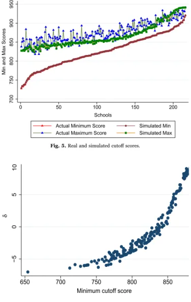
Fig. 4shows how different values of λ affect the fit of the model to the data for the Science high school nest. For each λ, the simulated minimum scores lie exactly on top of the actual minimum scores as depicted inFig. 4, a consequence of our estimation strategy. Thefigure shows the actual maximum score and simulated maximum scores forλ = 0.25, 0.5 and 1. Note how the lines move up asλ rises (or correlation falls) so that the extent of overlap increases.

We pin downλ using a simulation-based approach. The simulation algorithm works as follows: For a given vector λ, we obtain the vector δ( , ) and simulate the minimum and maximum cutoq λ ff scores, cj, andcj, for each school. Then wefind the vector λ that

best matches the actual maximum and minimum cutoff scores.

Simulating the error terms in the nested logit model creates some difficulties: taking a draw from the GEV distribution with the standard Markov Chain Monte Carlo Method is computationally intensive. We use a method proposed byCameron and Kim (2001) which takes a draw from the GEV distribution using a far less computationally intensive procedure.18

We draw M( = 100) sets of error terms εij for each student from the distribution function given in Eq.(1) by using the

parameters, λ. For each of the M sets of errors drawn, εk= 〈εijk〉,k= 1, ‥M, we allocate students to schools by using the placement rule.19_{After drawing each set of errors we get a distribution of scores for students in each school. Let g}

jkbe the set of scores in school

j in simulation k, ordered to be increasing20_:

Fig. 4. Real and simulated cutoff scores for λ = 0.25, 0.5, 1.

18_{This method is explained inAppendix A.1}

19_{We focus on the highest scoring 50,000 students to reduce computational intensity. The score of the student whose rank is 50,000 is lower than the minimum}

cutoff score of 216 schools and lower than the maximum cutoff score of all 226 schools.

20_{In the method proposed byCameron and Kim (2001), a change inλ only affects the coefficients. This allows us to keep the random seeds drawn from the extreme}

λ λ λ λ g_jk( ) = s ( ),s ( ), …,s ( ) j k j k jqk 1 2 _j

After ordering scores in ascending order for each school j and simulation M, wefind the expected value of the score for each rank within each school across the M simulations. The expected score of student with rank r in school j is thus:

∑

We take the lowest and highest ranked mean simulated score in each school. Wefind the λ that gives the least square distance between these simulated minimum and maximum cutoff scores and observed minimum and maximum cutoff scores. In effect, we are matching the maximum scores as the minimum scores are matched on average given our estimation procedure for obtaining δ:

⎛ ⎝ ⎜ ⎞ ⎠ ⎟

∑

∑

Table 1shows theλ values for each nest that minimize the distance between simulated and real maximum and minimum cutoff scores. As we mentioned before,λ is a measure of dissimilarity in preferences within a nest. If λ is small, students rank schools in the same nest according to their perceived quality( )δ so that students tend to agree on the ranking of schools. However asλ gets bigger, students differ in their preferences and no such ranking exists as their tastes for schools differ.

The correlation in shocks is low for vocational, teacher and local schools, suggesting that preferences are more horizontal there. This makes sense as these schools do not tend to be vertically differentiated: students usually go to the nearest one. As a result, the overlap in the support of scores in these schools is large which drives the high estimate forλ. The correlation is highest in the İzmir, Ankara, andİstanbul Anatolian high school nests (as λ is lowest). Note that the smaller the city, the higher the correlation in the city nest, as might be expected. In large cities, there may be enough schools so that students can choose the school that is most convenient without sacrificing much in quality. This would be picked up as greater horizontal differentiation, i.e., a higher λ. Science high schools are also more vertically differentiated than the others which again makes sense as they are the most elite of the schools. Thesefindings suggest, quite reasonably, that students' preferences are vertical for selective Anatolian and Science high schools, but less so for less selective vocational, teacher and local schools. Moreover, the standard errors are low so that the estimates are tight.21

The real and simulated cutoff scores for λ presented inTable 1are given inFig. 5. As we can see simulated maximum scores track the real maximum cutoffs quite well. Note that the actual maximum score is more variable than that estimated one. Heterogeneity in preferences comes from the error term. In our data we have no information about individual students preferences such as the school's location relative to their own home. As a result the error term ends up having more noise in it. For example, a very good student may choose a less selective Anatolian School just because it is close to where he comes from. This would raise the maximum score there above what the model predicts. If we had better information on students, we expect that we could do better at matching the maximum score.

Table 1 Nesting parameters: λ. Variable Coefficient λloc 0.958 (0.0001) λvoc 0.986 (0.0005) λank 0.795 (0.0007) λist 0.837 (0.0016) λizm 0.777 (0.0004) λteach 0.999 (0.0000) λsci 0.897 (0.0018)

Note: Standard errors are reported in parentheses.

Fig. 6depicts the relationship between the perceived valuation and the selectivity of schools. More selective schools clearly seem to be more valued. Close to the top of the score distribution a small increase in the score raises utility a lot while a similar increase at low scores has little effect. In the next step, we investigate the factors affecting the students' perceived valuations of the schools. 3.4. What drives valuations?

Once we pin down the λ that gives the best match of the actual and the simulated cutoffs, we get δl( ,q λl . Returning to the) definition of δ, the vector of mean valuations for schools,

δl=βX+ξ (2)

where X is the observed characteristics of the school, andξ is the school specific component of mean valuations. ξ is the unobserved, common across all agents, school specific preference shock. X includes the school's success on the ÖSS the previous year, its age/ experience, type, education language, dormitory availability, whether it is located in a big city (Ankara,İstanbul, or İzmir), the number of seats, and the cutoff score of the school. Agents may value selectivity, i.e., a high cutoff score, for the associated bragging rights and/or because they use it as a signal for unobserved quality. The cutoff score is an equilibrium outcome and so endogenous by definition. The dummy for being a Science or Anatolian high school incorporates the possibility that such schools have a good reputation and this makes people value them. This could be for consumption purposes, perhaps for the bragging rights associated with going there.

The cutoff score is an equilibrium phenomenon. An increase in the valuation (though any of the channels that people seem to care about) will shift demand out and raise the cutoffs. An increase in the number of seats will both change the valuation (if agents

Fig. 5. Real and simulated cutoff scores.

care about the school size) and so shift demand and raise the cutoff. It will also directly affect supply so that the cutoff will fall.22

We allow valuations to depend on a number of factors, including the cutoff score itself.23_{The equilibrium cutoff is then a fixed}

point: given the equilibrium cutoff, valuations generate the same cutoff in equilibrium. In Eq.(2)there is a valuation shock,ξ, which acts as the error term. There is thus an econometric issue associated with including the cutoff score as an explanatory variable.24

Ifξ, the school specific valuation shock, is large and positive, then the cutoff score will be high as well, so that the cutoff will be correlated withξ. This will bias the estimates of β obtained upward. This is the familiar endogeneity problem. To deal with this we need good instruments for the cutoff score. We partition X as X c[ , ]͠ so that

δl=β∼X͠ +γc+ξ

A good instrument is an exogenous variable that shifts the cutoff score, but does not affect a school's average valuation δ directly. The first variable that comes to mind that shifts the minimum cutoff score is the number of available seats in a school. However, the available number of seats may affect the valuation of the school directly. In addition, it may be a response to a highξwhich makes it less than optimal.25_{Fortunately, the model suggests which instruments to use for the minimum cutoff score. Next, we explain what}

these are and how we construct them, and then present our results.26

The model predicts that the number of available seats in schools worse than a given school has no effect on the demand for the school. However, the number of seats in better schools does affect demand: more seats in better schools are predicted to reduce the cutoff score of a school. This comes from the observation that the demand for a school comes from those who like it the most, from the alternatives that are open to them. Changing the cutoff in worse schools has no effect on the alternatives open to a student going to a better school, and hence, on their demand. In other words, if Podunk University offers more seats, there is no effect on the demand for Harvard since everyone choosing to go to Harvard had, and continues to have, Podunk in their choice set. But if Harvard offers more seats, it may well reduce the demand for Podunk University. It could be that someone chose Podunk because they could not get into Harvard. Once Harvard increases its seats and so reduces its own cutoff, Harvard may become feasible for such a student. As we use seats in other schools to instrument for a school's cutoff we need not worry about any correlation with ξ.

To construct the instrumental variable, we need a ranking of schools free ofξ. We will use the schools' success on the verbal and quantitative part of the ÖSS in the previous year to rank schools.27_{We construct our instrumental variable as follows:}

1. For each school, wefind the schools that have better average test scores in both dimensions, verbal and quantitative.

2. Wefind the total number of seats in all of the schools found in step 1. The available number of seats in the school itself is not included. The second set of instruments we use is constructed using a different insight. A large positive draw ofξ, the school specific demand shock, would raise demand for the school and so raise both the minimum score and the maximum score. As a result, the residual from the regression of the minimum cutoff score on a flexible form of the maximum score will be correlated with the minimum cutoff, but orthogonal to the school specific demand shock,ξ. This makes it a good instrument.28_{We thus use the residual}

of the minimum score on a polynomial function of maximum score as an instrument for the minimum cutoff score29

: c=λ0+λ c1 +λ c2 2+ν

Table 2shows ourfirst stage estimation: c=ηX͠ +κ1*Seats in better schools +κ ν2* +l ε

Note that the number of seats in better schools has a negative coefficient: more seats in better schools reduce the school's own cutoff as expected. The second instrumental variable, the residual from the regression of minimum cutoff on a polynomial function of maximum score, has a positive coefficient as expected since the minimum score would be increased by a positive shock as captured by a positive residual.

Finally, according to the model, the number of seats in worse schools should have no effect on the school's own cutoff.Table A8 presented inAppendix A.3shows thefirst stage estimation after adding as an additional instrument the number of seats in lower scoring schools. As expected, this additional instrument is not significant. We also test for the exogeneity of the cutoff score using a Hausman test and reject the hypothesis with p-value equal to 0. Our model is overidentified. According to the results of heteroskedasticity-robust score test (Wooldridge, 1995), we cannot reject this hypothesis with p-value 0.17.

22_{The net effect will be negative if the equilibrium is stable.}

23_{This is like putting in the price into the utility function: people get utility from the price being higher in a Veblenesque manner.}

24_{The same criticism might be thought to apply to variables like the school's average score in (parts of) the university entrance exam. However, it is far from clear}

why this would happen. Even if class quality today rose with the cutoff, this would only affect university entrance exam results with a 3year delay.

25_{This is less of a concern in Turkey, where the number of seats is usually equal to the size of the graduating class as the overall school size is set by the central}

authority and can be thought of as exogenous.

26_{An exogenous change in the cutoff score could occur if it was misreported by accident and last years cutoffs affected this years valuations.}

27_{Of course, there could still be a problem if demand shocks when the students in the previous year were admitted was strongly serially correlated with today's}

demand shock. As long as the correlation between the demand shock today and at the time the students in the previous year were admitted are small, our instrument is valid.

28_{One might ask what could affect the maximum score and not the minimum score. The score distribution around the cutoff score of a school does not affect its}

maximum score but it affects its minimum cutoff score.

Thefirst column ofTable 3shows our baseline estimates, where we regress average valuation on the exogenous variables and do not include the minimum cutoff score of a school. This column suggests that past performance on the university entrance exam (ÖSS scores) and school type drive preferences. The second column ofTable 3shows the results of the regression of the average valuation on the exogenous variables and the school's cutoff score. The coefficient on the minimum score is positive and highly significant suggesting that a more selective school is highly valued. The significance of past scores on the university entrance exam are less significant, as would be expected given that the cutoff is positively correlated with the past performance of a school so that including it picks up some of this variation. However, as explained above, cutoffs are not exogenous. As cutoffs are high when the school preference shocks are high, cutoffs are positively correlated with the error term which imparts an upward bias to the coefficient. The third and fourth columns show the results when we instrument for cutoffs. The third column reports the 2SLS estimates, and the fourth column reports the limited information maximum likelihood (LIML) estimates. The latter has better small sample properties. It is reassuring that the estimates from both methods are very similar. In addition, note that after instrumenting for the cutoff score, the coefficient on it falls (as expected) but remains positive and significant. Past performance on the university entrance exam becomes more significant suggesting that, conditional on the cutoff, a school's performance on the university entrance exam is an important determinant of its valuation. Thus, students do look at how well students graduating, or the output of a school, in forming their valuation of a school. These results are consistent with thefindings ofBurgess et al. (2009)andHastings et al. (2008)who reach a similar conclusion using data from the Millennium Cohort Study in the UK, and school choice data from the Charlotte-Mecklenburg School District, respectively.30

Anatolian high school inİstanbul 24.090

(19.870)

Anatolian high school inİzmir 13.460

(20.850)

Education language– English 11.410

(11.160)

Education language– German −3.628

(11.810) Dormitory availability 13.140 (6.895) Ankara 26.46* (12.690) İstanbul 23.780 (14.750) İzmir 30.93* (15.110)

Seats in better schools −0.00358*

(0.002)

Residual from min regression 0.740***

(0.087)

Constant 708.2***

(35.050)

F-stat (Excluded variables) 41.512

R2 _0.802

N 161

Note: Standard errors are reported in parentheses.

*_{Significance at the 0.90 level.} **_{Significance at the 0.95 level.} ***_{Significance at the 0.99 level.}

30_{The significance level of the “seats in better schools” instrument is lower than the “residual from min regression” instrument. One might wonder whether our}

Science high schools and schools inİstanbul, Ankara, and İzmir are also valued beyond what they would be based on their selectivity alone. As mentioned before, Science high schools are very prestigious. It could be that attending such schools gives one contacts in the future as well as a consumption value in the present.MacLeod and Urquiola (2009)show that a school's reputation can affect wages as the identity of the school attended gives information about a student's ability. This could also rationalize the high valuation placed on Science high schools. It could also be that the high valuation of Science high schools comes from the students' use of school type as a proxy for school quality. In the next section we look at the value-added of each Science high school by estimating the effect or the value added of the high school on their students' performance on the university entrance exam. 4. Value-added by high schools

In the previous section, we estimated the preference parameters and simulated the high school entrance exam scores for students in each school. We allocated students to schools on the basis of the estimated preference parameters and the overall score distribution using simulations. In this section, we estimate the value-added by a school in terms of their students' academic performance. Here we are limited by the data. We do not have a panel, so we cannot match the score the student obtained on the high school entrance exam to what he obtained on the university entrance exam. Rather, we infer the effects of schools on student performance by comparing the mean high school entrance exam (OKS) score to the mean university entrance exam (ÖSS) scores for each school. We have many years for the latter, but only one year for the former. We estimate the average value added per school by running a regression of the difference in the (standardized) mean score of a school in the university entrance exam and in the high

Table 3

School choice: estimation results.

Variable (OLS) (OLS) (2SLS) (LIML)

Number of available seats 0.005 0.00842* _{0.007 0.007}

(0.007) (0.004) (0.004) (0.004)

Average quantitative score in 2000 ÖSS 0.218*** _0.0680* _0.116** _0.117**

(0.053) (0.033) (0.036) (0.036)

Average verbal score in 2000 ÖSS 0.306*** _0.0865* _0.157*** _0.159***

(0.053) (0.038) (0.039) (0.040)

Age 0.026 0.032 0.030 0.030

(0.062) (0.031) (0.040) (0.040)

Science high school 8.422*** _3.237*** _4.892*** _4.936***

(1.764) (0.765) (1.034) (1.047)

Teacher high school 4.039* _{0.867 1.880 1.907}

(1.931) (0.763) (1.063) (1.075)

Anatolian high school inİstanbul 1.928 −0.544 0.245 0.267

(2.152) (0.728) (1.156) (1.169)

Anatolian high school inİzmir 1.715 0.392 0.814 0.826

(2.280) (0.679) (1.036) (1.050)

Education language– English 2.671 −0.028 0.834 0.857

(2.192) (1.118) (1.418) (1.429)

Education language– German 1.198 0.330 0.607 0.615

(2.254) (1.175) (1.458) (1.467) Dormitory availability 1.617 0.500 0.856 0.866 (0.893) (0.455) (0.555) (0.558) Ankara 4.235** _{0.733 1.851}* _1.881* (1.494) (0.485) (0.784) (0.795) İstanbul 4.485*** _1.687** _2.580** _2.604** (1.297) (0.522) (0.771) (0.779) İzmir 3.746* _{0.608 1.610}** _1.637** (1.449) (0.381) (0.580) (0.591)

Minimum cutoff score 0.0846*** _0.0576*** _0.0569***

(0.006) (0.007) (0.008)

Constant −22.95*** _−76.18*** _−59.19*** _−58.73***

(3.121) (4.363) (4.596) (4.654)

R2 _{0.807 0.942 0.928 0.927}

N 161 161 161 161

Note: Corrected standard errors are reported in parentheses.

*_{Significance at the 0.90 level.} **_{Significance at the 0.95 level.} ***_{Significance at the 0.99 level.}

(footnote continued)

εij ij i i fic and individual specific components of

the university entrance exam score shock and are independently distributed, mean zero error terms. Thus si =α +ε hs i i hs and

⏟

where j indexes schools andγjis the school value-added. Assume that α γ u vi, j, j, i c

andεihsare independent of each other. The school

level common shock, uj, is a shock affecting the performance of all students in the school. εihsand viccan be thought as idiosyncratic

shocks such as air pollution (Ebenstein et al., 2016) or the noise level near where students take the exam (students take both exams in schools that they are assigned randomly in a city that they prefer) that affect performance, but are uncorrelated with other observables. We do not observe the individual students' scores, but only the school level average scores for the university entrance exam. Thus, aggregating to the school level in the model above, we get the mean scores in the OKS and ÖSS from school j:

E s(i | ) =j E α j( ) +E ε( | )j hs i i hs and E s j t( | , ) =ijc E α j t( i , ) +γj t, +E ε j t( | , )ijc

The t is the time index as we have more than a single year's data on the university entrance exam. Under the following assumptions, we can get a consistent estimate of the school value-added, γj t,, by using the data on the performance of the schools over time.

Assumption 1. E ε j(i | ) = 0

hs

.

Assumption 1is a heroic one and is unlikely to hold in the data we have. Students with better scores, and hence with better shocks to their scores on the high school entrance exam, get into a better school while those with worse ones do not. As a result, it is expected that the mean scores of students in the best (worst) high schools will look like they have fallen (risen) in the university entrance exam even if there is actually no value-added by any school. This is the familiar mean reversion issue. All we are saying here is that ifAssumption 1holds, then we can easily estimate value added. If it is grossly untrue, then our estimates will be biased due to mean reversion and we will need to correct for this.

Assumption 2. E α j t( i , ) =E α j( i ) ∀t.

Assumption 2states that students placed in a school have the same ability on average over time. This is a reasonable assumption in the Turkish system. The cutoff scores are fairly stable as the educational environment in Turkey has been unchanged over the last few decades. InAppendix A.2we present evidence on the stability of cutoff scores.

Assumption 3. γj t, =γj∀t.

Assumption 3says that school value-added is time-invariant.Assumptions 1–3imply that the variation in the performance of a school comes from the shock, ujt, received by that school in that year.

Under these assumptions the average performance of students in school j at time t can be written as E s j t( | , ) =ij E s( | ) +j γ +E u( +v j t E s j t| , ) ( | , ) −E s( | ) =j γ +E u j t( | , ) c i hs j j i c ij c i hs j j

To account for the correlation in the shocks received by a school over time, we cluster standard errors at the school level. Value added modeling has become a key tool in the attempt to evaluate teachers and institutions, especially in the US, seeKoedel et al. (2015)for a useful survey of recent work. Two papers stand out in this literature.Chetty et al. (2014a)use value added modeling to monetize the gains that would occur from improving teachers using Internal Revenue Service (tax) data. Their work

suggests that these gains are large: replacing a teacher in the bottom 5% in terms of value added with an average one would raise the present discounted value the earnings of all students in the class by $250,000. However,Rothstein (2015)criticizes these estimates as being biased due to unobserved sorting. His argument is elegant and devastating. He shows that after adding the usual controls, current student test score growth is correlated with future teacher value added, suggesting that student assignments to teachers are not random. However,Chetty et al. (2015)argue that future value added is generated from past student scores leading to a mechanical correlation noted byRothstein (2015).32

Deming (2014)also points out that only controlling for prior test scores may not be enough to control for sorting across schools so that value-added estimates will be biased. In our framework, if students with better (worse) unobserved characteristics sorted into more (less) selective schools our value-added estimates would be upward biased for more selective schools and downward biased for less selective schools. There is also considerable controversy over the persistence of teacher value added and on the viability of using such measures to incentivize students. After all, if teachers are judged by a given yardstick, they will naturally direct their efforts to look good according to the yardstick (perhaps by teaching to the test rather than encouraging understanding of the material) with long run costs.33

4.2. Results

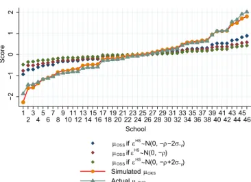
Before we present our results, we examine the patterns in the data on the schools' average performance on the university and high school entrance exams, to understand the effect of noise on the average performance of schools. The patterns seem to be driven by ability sorting, value added, and mean reversion. We normalize the average ÖSS score and the average OKS scores so that they have mean zero and variance of unity.

Looking at the patterns in the data we see that there seems to be a role for ability in the sorting between schools. If ability did not affect the scores on the high school and the university entrance exams, then allocation of students to schools would be independent of ability. In that case, the correlation between the (normalized)average ÖSS score and the average OKS score would be zero if there is no value-added by schools. If there was value added by schools, and this mattered to students, then the high value added schools should be harder to get into and sorting by ability should occur. The correlation and rank correlation of these mean OKS and the mean ÖSS scores are strongly positive as inTable 4 and 5suggesting some sorting by ability.

If there was sorting on the basis of ability and/or preferences, no value-added by any school, and no randomness in OKS scores, we would expect the normalized OKS and ÖSS scores to lie along the 45 degree line. When we plot normalized OKS and ÖSS scores as inFig. 7, thefitted line is flatter than the 45 degree line, which is in red. This should not be taken to mean that more selective schools have negative value added as this could arise from mean reversion if there was randomness in the OKS scores.

The less the randomness in the OKS score relative to the variation in ability, the more informative is the high school entrance exam score and the lower the extent of mean reversion bias. If we knew, or could assume something about the variance in the OKS score, we might be able to pin down the value-added by a school.

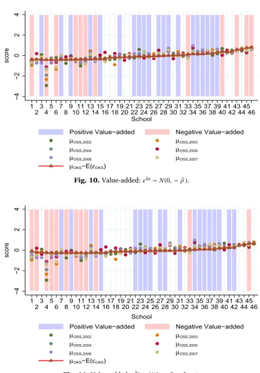
Fig. 8presents the same data in a slightly different way. It orders schools on the basis of their cutoffs, not the average score, with School 1 being the least selective one. Thus, the schools are ordered from“worst” to “best”. Each school's score on the university entrance exam from 2002 to 2007 as well as the high school entrance exam score in 2001 is plotted. The high schools whose normalized ÖSS scores are significantly higher than their OKS ones, i.e., those with positive “value-added” are highlighted in blue, while those with significantly negative “value-added” are highlighted in red. No highlight means the estimated value-added is not significantly different from zero. Note that the value added here is contaminated by mean reversion.

The least selective schools seem to add value on average and the most selective ones seem to reduce it, although School 4, one of the worst schools, reduces value. As discussed above, this broad pattern could be just a reflection of mean reversion. In the next section, by using auxiliary student level data from a school, we estimate the magnitude of the mean reversion bias and correct for it.

4.3. Mean reversion bias

In the previous section we noted that the mean difference in school performance in the OKS and ÖSS exams captures both mean reversion and value-added. In this section, by using auxiliary student-level data we were able to obtain for only one school, we develop a way to correct for the bias due to mean reversion. This auxiliary data contains each student's name, their high school score and their college entrance exam score. This school (which is not a Science high school, but is an Anatolian exam school) has roughly the same cutoff score as the one with rank 16 inTable 4.34

As in the previous section, we normalize scores within this Anatolian exam school so that the mean score is zero and its standard deviation is 1 on both exams. If the value-added by a school is constant across students35then student i's high school and university entrance exam scores are given by36

32_{There is an ongoing debate on this issue, seeChetty et al. (2014a,b, 2015),Rothstein (2015), andBacher-Hicks et al. (2014).}

33_{This is well understood in the principal agent literature as the optimal contract may be to not provide high powered incentives for easily measured outcomes. For}

example, tying remuneration of CEOs to stock prices may cause them to direct their efforts to short term projects rather than long term ones that build value.

34_{This is the only school that posted incoming students OKS scores as well as their OSS scores when they graduated on its website.}

35_{This is a strong assumption. A school may add positive value to some students and not to others as inDuflo et al. (2011). However, if this assumption fails to}

hold, we cannot account for mean reversion in our data.

Rank of mean score OKS ÖSS 2002 ÖSS 2003 ÖSS 2004 ÖSS 2005 ÖSS 2006 ÖSS 2007 OKS 1 ÖSS 2002 0.8341 1 ÖSS 2003 0.8191 0.7988 1 ÖSS 2004 0.8347 0.8228 0.8533 1 ÖSS 2005 0.7438 0.6365 0.7479 0.8013 1 ÖSS 2006 0.8758 0.8171 0.8971 0.8927 0.7968 1 ÖSS 2007 0.851 0.7983 0.8489 0.87 0.7754 0.8825 1

Fig. 7. Average ÖSS score by average OKS score. (For interpretation of the references to color in thisfigure, the reader is referred to the web version of this paper.)