ISTANBUL BILGI UNIVERSITY
INSTITUTE OF SOCIAL SCIENCES
INTERNATIONAL FINANCE MASTER’S DEGREE
PROGRAM
PORTFOLIO CONSTRUCTION WITH PARTICLE SWARM
OPTIMIZATION IN TURKISH STOCK MARKET
Ozgur SALMAN
114665013
Supervisor: Assoc. Prof. Dr. Cenktan ÖZYILDIRIM
ISTANBUL
ii
ACKNOWLEDGEMENT
I would like to express my sincere gratitude to Assoc. Prof. Dr. Cenktan Özyıldırım for his guidance at every level of my improvement in the field of finance.
I would also like to dedicate this work to my mother and sister.
iii
ABSTRACT
This study serves as an experimental approach to portfolio selection with using a particle swarm optimization technique. PSO is used as an integration of social behaviors into a portfolio optimization problem. With integration of PSO, returns of financial asset has a chance to be treated as mathematical reasons to a cognitive surface. The main objective is to maximize the expected return and minimize the risk as of the variance via the MATLAB software. To detect analogous results by another traditional portfolio selection models, other portfolio optimization techniques are implemented into code. Code is constructed by the main pso script and six other function scripts. Study data consists of six stocks which are participants of BIST 30 index and it is tested through the December 31st of 2010 to December 30th of 2015. As a comparison, mean-variance model and particle swarm optimization are compared. Main problem with the mean-variance model, it puts the weights on two criteria only and contains no implementation of short selling. On the contrary, PSO is seemed to be a favorable technique to implement a weight adjustment to a portfolio in the unconstrained search space.
iv
ÖZET
Bu çalışma, parçacık sürü optimizasyon tekniği kullanılarak, portföy seçimi için deneysel bir yaklaşımı sunmaktadır. PSO, sosyal davranışların bir portföy optimizasyon problemine entegrasyonu kullanılmıştır. PSO'nun entegrasyonu ile finansal varlıkların getirileri, matematiksel nedenler olarak, algısal düzeyde ele alınma şansına sahiptir. Temel hedef, MATLAB yazılımını kullanarak, beklenen portfolyo getirisini maksimize etmek ve aynı zamanda portfolyo riskinin varyansını en aza indirgemektir. Birbirine benzer başka geleneksel seçim modellerini tespit etmek için, diğer portföy optimizasyon teknikleri koda uygulanmaktadır. Kod, ana pso komut dosyası ve altı diğer fonksiyon dosyası tarafından oluşturulmuştur. Çalışma verileri BIST 30 endeksinin katılımcıları olan altı hisse senedinden oluşmaktadır ve 31 Aralık 2010'dan 30 Aralık 2015'e kadar test edilmiştir. Bir karşılaştırma olarak, ortalama-varyans modeli ve parçacık sürüsü optimizasyonu karşılaştırılmıştır. Ortalama-varyans modelinin temel problemi, ağırlıkları yalnızca iki ölçüt üzerine dağıtmaktadır ve kısa satış uygulaması içermemektedir. Aksine, PSO sınırlandırılmamış arama alanında, portföye ağırlık dağıtımı yapmak için daha uygun bir teknik gibi görünmektedir.
v
TABLE OF CONTENTS
ACKNOWLEDGEMENT……… ii ABSTRACT……….. iii ÖZET………. iv TABLE OF CONTENTS……….. v LIST OF FIGURES………. viLIST OF GRAPH………... vii
LIST OF TABLES………. viii
1. INTRODUCTION……….. 1 2. LITERATURE REVIEW……….. 4 2.1. Evolution of PSO………... 4 2.2. Overview of PSO………. 23 2.3. Topology in PSO………. 25 2.4. PSO on finance……… 29 2.5. Applications of PSO……… 30
3. DATA AND METHODOLOGY………. 31
4. IMPLEMENTATION OF MEAN-VARIANCE MODEL………... 41
5. IMPLEMENTATION OF PSO MODEL……….. 45
6. COMPARISON OF PORTFOLIOS………...54
CONCLUSION……… 62
vi
LIST OF FIGURES
Figure 2.1: Boids Movements by Different Parameters……… 7
Figure 2.2: Applied Rules for The Game of Life……….. 10
Figure 2.3: Crossover Patterns……….. 13
Figure 2.4: Mutation Pattern………. 14
Figure 2.5: Inversion Pattern………. 14
Figure 2.6: Original PSO Scheme……….. 23
Figure 2.7: Ring Topology……….. 25
Figure 2.8: Fully Informed Particle Topology……….. 26
Figure 2.9: Star Topology………... 27
Figure 2.10: Mesh Topology………... 28
Figure 2.11: Toroidal Topology………. 28
Figure 2.12: Tree Topology……… 29
Figure 3.1: Return and Risk Relation………... 37
Figure 4.1: Code of Data Implementation in Mean-Variance Portfolio……… 41
Figure 4.2: Code of Asset Moments and Portfolio Constraints……….. 41
Figure 4.3: Code of Comparison to Sharpe Ratio……… 41
Figure 4.4: Code of Risk and Return……… 42
Figure 5.1: Code of Cost Function and Population Limits……….. 45
Figure 5.2: Code of Main Approach and Limits……….. 46
Figure 5.3: Code of Particle Initialization……… 46
Figure 5.4: Code of Velocity Initialization and Catcher………. 47
Figure 5.5: Code of Updating the Velocity and Position………. 47
Figure 5.6: Code of Convergence……….. 48
Figure 5.7: Code of Updating the Personal Best and Catcher……… 48
vii
LIST OF GRAPH
Graph 3.1: TUPRS, OTKAR and KOZAL’S Monthly Prices……… 32
Graph 3.2: TUPRS, OTKAR and KOZAL’S Monthly Returns……… 32
Graph 3.3: THYAO, GARAN and ARCLK’S Monthly Prices……….. 33
Graph 3.4: THYAO, GARAN and ARCLK’S Monthly Returns………... 33
Graph 3.5: BIST 30 Index……….. 34
Graph 4.1: Weights Distributed to Stocks……… 42
Graph 4.2: Efficient Frontier of Mean-Variance Portfolio………. 43
Graph 4.3: Capital Allocation of 3 Stock Simulation……….. 44
Graph 5.1: Weights Distribution by Stocks in Each Solution……… 49
Graph 5.2: Efficient Frontier in First 6 Solution………. 51
Graph 5.3: Efficient Frontier in Last 9 Solution……….. 52
Graph 5.4: Efficient Frontier for Portfolio………... 53
Graph 6.1: Return Distribution by Stocks in 2016 from Mean-Variance…………..54
Graph 6.2: Return Distribution by Stocks in 2017 from Mean-Variance…………..55
Graph 6.3: Return Distribution by Stocks in 2016 from Risk Minimized…………..56
Graph 6.4: Return Distribution by Stocks in 2017 from Risk Minimized…………..57
Graph 6.5: Yearly Returns by Portfolios………...58
Graph 6.6: Stock Returns in 2017 from Mean-Variance Portfolio……….60
Graph 6.7: Stock Returns in 2017 from Minimized Risk Portfolio………61
viii
LIST OF TABLE
Table 2.1: Functions Applied to Comparison………...21
Table 2.2: Applications of PSO in Real World……….30
Table 5.1: Weights in Each Solution………..50
Table 5.2: Optimal Risk in First 6 Solution………...51
Table 5.3: Optimal Risk in Last 9 Solution………....52
Table 6.1: Monthly Returns in 2016 from Mean-Variance………..54
Table 6.2: Monthly Returns in 2017 from Mean-Variance………..55
Table 6.3: Monthly Returns in 2016 from Minimized Risk PSO………56
Table 6.4: Monthly Returns in 2017 from Minimized Risk PSO………56
Table 6.5: Monthly Returns in 2016 from Maximized Return PSO………...57
Table 6.6: Monthly Returns in 2017 from Maximized Return PSO………...57
Table 6.7: Portfolio Weightings by Mean-Variance Portfolio……….59
1
CHAPTER 1
INTRODUCTION
In the field of finance, portfolio selection is highly deep and most tempting concept for a researcher from the first day Markowitz (1952) gave a clear identification to a topic which is a major decision-making process that everyone of us related to. The other improvement to portfolio construction topic is suggested by Tobin (1958), study proposed an idea of Keynesian portfolio which is selected either bonds or cash. Over the decades, as the investable instruments has risen, money supply has increased along with it. For a brief demonstration, balance sheet size of Federal Reserve System of United States and European Central Bank has risen drastically in the 21th century. Between 2003 and 2017, growth in the total assets of FED and ECB are 720,1 million USD to 4,437 trillion USD and 795 million Euros to 4,440 trillion Euros, respectively.
Naturally, in the world of an increasing Money supply, decision–making processes on portfolio construction and investment instrument selection are highly demanded research subjects to focus on.
In the early phase of the subject, comparative solution to a selectional investment decisions had a lack of computerized speed. By the mean of speed absence, it can be visualized with a hypothetical example. Imagine a foreign investor who wants to purchase a rice field in Japan in the 60ties. Also, investor in an attempt to hedge his long position against an undesirable outcome from precipitation. Even with an adequate data collection, which was also another difficult topic at that time, from the previous meteorological data investor could barely process this data into a possible outcome in days.
2
The other puzzled complication is the gathering the data, again from the rice investor example, only helpful variable to use in the simulation is data that were connected to Japan individually. However, rice price’s dependence should be on the global equilibrium, which is forced by every individual around the world who is sided as a producer and also a consumer. From the logic of the absence of accessible data other than the investee country, simulation would be limited to Japan’s outcomes only.
Over the decades, alongside the progress in the technological area, accessibility of the individuals to different financial instruments and information have rised exponentially. With this enormous rise in the transferable knowledge or awareness, cognitive surface of the human has become indifferent between the choices time to time. For the purpose of investigating a pick for investment decision, traditional approaches have become impractical at large.
Main problem with the conventional paradigm is it lacks the social behavior part. Appraising every individual selection separately from one another as if it does not hold connection to the other parts or to a whole, skips the idea that destination is a cumulative experience and information gathered jointly.
Enlightenment to singular decision-making progress on investments, each choice can be emphasized as a particle which desires to find the best option possible in the terms of returns. Also, the possible choices that can be achieved in the finite variation can be seen as a search space.
As an optimizer for a best solution in the search space, Particle Swarm Optimization is introduced to the academic discussion “A New Optimizer Using Particle Swarm Theory” in 1995. Following advancement to the subject have been published throughout the years.
In adapting PSO to portfolio construction, each investment decision composes of three dimensional vectors. Every individual particle composed of three dimensional vectors. First one is the current position ‘x’, second one is previous
3
best position achieved through the search space ‘p’, and the third one is the velocity which is denoted by the ‘v’. The current position x presents a set of coordinates that illustrate a discrete point in space. Each succeeding iteration in the algorithm, current position is appraised as a solution. In the terms of a possibility that if the sequent position reaches the levels that has not been found so far, then the new position ascertained as local best and stored in the vector p. The value of the best function accordingly to new “p” is stored in a variable which is called “pbest” (represents previous best) and it can use for comparison on later iterations.
The purpose is to keep reaching the unattained level of positions that serves as a better feeder and accordingly updating the positions which are derived from this new position. To obtain a new position, algorithm is adjusted constantly by adding v coordinates to x.
4
CHAPTER 2
LITERATURE REVIEW
2.1. Evolution of PSO
Before jump to the late 20th’s century researches which had numerous privileges backed and tested their data by computer, one of the topic that needs to be mentioned is how observations transform into algorithm. That remarks which were materialized in the early 20th. century are the auxiliary force behind the standard PSO.
Study of cumulative knowledge that gathered as a flock of birds in the animal world, first acknowledged by Selous (1931). The idea of ‘thought transference’ between the members of flock is one of the columns’ in a ‘observations to hypothesis sided by data’ era. In order to support his conclusion, he referenced the simultaneous rise of a flock without obvious extraneous impetus; moment of sudden silence at the time colony of terns screams.
In his findings, author’s reflections upon each observation bring up the question of if it is a subjective conclusion or a scientific fact. However, under the scrutiny on the issues of ‘leader’ and ‘sentinel’ phenomena showed that these beliefs once held were illogical and improbable at least. In the absence of pompous character to lead in the flock or a guard system to control the group, connectivity between the swarm should be achieved via ‘thought transference’ he aimed to disclose. “What, with us, is rational intercourse, with conversation, which probably weakens emotion, may be with birds in numbers a general transfusion of thought in relation to one another, on the plane of bird mentality--such thought corresponding more to our feeling than to what we call such, for it is out of feeling, surely, and not vice versa, that thought has evolved. This, then, may be the great bond between individuals of a species, probably acting through a
5
sensation of well-being in one another's society which, when well developed, leads to gregariousness in rising degree.”
On the contrary, capability of the human eye on noticing these simultaneous extreme transference is still doubtful. Even though, Selous backs his case with instances that spreading through the flock, why some are movements of individuals imitated by the group, while other movements are avoided by the majority? is another question needs some clarification.
Selous’ findings and presumptions are the supplementary work to reach the understandings of a control mechanism and ‘thought transference’ seemed as a way of telepathic framing to the center of knowledge that spreading to each individual in the flock. Although, without arithmetic background, simulations via testable data and modelling, observations from human sense would remain an ambiguous assumption by the applicant still his aim to correspond each individual to a flock and see as if they are the participants of one big group which reacts and acts simultaneously is a column to swarm optimization.
Reynolds (1987) explored an approach based on simulation to script the paths of each bird individually. The gathered motion of the simulated flock created by a distributed behavioral model according to appliance for a natural flock. In his research, each individual bird had a chance to choose their own path and each one of them has an independent course from another. Also, they manoeuvre, go up-down, change their direction in agreement with their local perception of the dynamic environment. Potts’ (1984) evidence of “The chorus-line hypothesis of manoeuvre coordination in avian flocks” supports the idea of centralized mechanism to transformative knowledge between the flock’s members. On the contrary to leadership phenomena, although, individual bird may trigger a manoeuvre which spreads through the flock in a wave, initialization of this ‘manoeuvre wave’ begins passively but its mean speed has three times higher than the scope of it would be possible if birds are simply reacting to their adjacent neighbours. Hypothesis suggests any bird starts the manoeuvre but the
6
coordination to achieve is transferred in the flock via visual communication and this can be seen as a supportive idea that there should be control mechanism to transform the knowledge to each individual.
Reynolds’ research sided the idea of each individual bird has their discrete motion and yet overall motion of flock is synchronized and fluid. Hence, the simulation brings down the curtain of centralized control. All his evidence supports the idea of flock acts as an organism that its actions resulted by the individuals’ behavior from their local perception of the world.
Computer simulation and modelling are the main force behind the Reynolds’ adventure. Its aim to capture the individuals behaviour and movements as they have complex shape other than rigid figures are groundbreaking. Also, attribution of each individuals are part of the simulation, which is the main step towards the study of these individual as they are particles. Reeves (1983) proposed a technique for modelling a class of ‘fuzzy objects’. Paper represents a model that ables to track the motion, changes of form, and dynamics via the attribution inputs. Particles in his paper, generated by their attribution of:
• Initial position,
• Initial velocity (both speed and direction), • Initial size,
• Initial colour, • Initial transparency, • Shape,
• Lifetime.
Reeves research is differentiated from the other particle modellings study by its aim to capture the complex shape existence such as ocean wave, cloud, fire, or smoke. Also, representations vary in propositions such as particle system is not a
7
static entity and it has a duration. Moreover, an object in a particle system is not deterministic, instead, it has a stochastic root to create an appearance. The conclusion that serves in Reynolds’ simulation in a didactic way is particle systems are stochastic images and controlled by several global parameters.
Figure 2.1: Boids Movements by Different Parameters
Dot’s or spheres are illustrated as a single atomic particle in Reeves’ research but Reynolds replaced them to boids in order to capture visual connotation and further apprehension in the fractional level as in a flock. The other supplementary work of the boid is to chase the behavior of its movement in more complex surface. Also, particles hence boids interact each other which allows to examine the
8
internal state and also external state of boids. This is a major difference from a Reeves’ model which its particle does not connect to one another.
To replicate the real flight ‘geometric flight’ is used by Reynolds. In real flight, continues moving actions take a part simultaneously, however, geometrical flight is considered to be small linear motions to reach a curve path. The other considerable subject in the simulation is ‘momentum’. In framing the momentum, research points out if object in a flight it tends to have a desire to flight. The other argument is limitation of speed and acceleration, there is maximum speed that boid can achieve and also a limit to minimum speed which defaulted zero. Likewise, acceleration’s maximum limit is narrowed to a fraction of maximum speed to smooth the changes in the speed and direction.
Other than a gravital force many physical forces are skipped in simulation such as friction forces. In the absence of essential forces, gravitational force counters and aligns with the buoyancy and aerodynamic lift, respectively.
In the phase of characterizing and modelling a flock from a singular element, boids in this research, adding behavior to them is used by Reynolds. These behaviors:
• Collision Avoidance: avoid collisions with nearby flock mates.
• Velocity Matching: attempt to match velocity with nearby flock mates.
• Flock Centering: attempt to stay close to nearby flock mates.
As a vector, velocity includes both the heading of boid or direction of it and its speed. Definition of nearby is one of the highlighted situation needs to be discussed. Study implements the idea of one boid’s awareness can be quantify by
9
how much the proximity lies down between the neighbour boids and the main boid.
Reynolds suggests, while one boid attempt to match velocity with nearby flock mate, at the same time, it tries to avoid collision with the nearby flock mate so that these two-behavior complementary to one another. From the logic of it, velocity matching ignores position and collison avoidance ignores velocity conversely. For instance, if the boid reaches the velocity of its neighbour, it is unlikely to collide with its neighbour any time soon.
The other behavior of boid that implemented by the study is centering, when boid desire to be around the center of the flock. Also, this centering behaviour gives a boid to direction that fly accordingly to centroid of the nearby flock mates.
The concluded idea from Reynolds’ simulation gives a guidance to a deeper understanding of a particle when it is backed by different behaviour. From Reeves suggestion to test the particle by its own attribution with the input of varied from one another, Reynolds visualizes noncolliding aggregate motion. Also, his assumption of each boid or bird works independently has significant contribution to idea of transitive knowledge between particles.
Hepner and Grenander (1990) research’s suggests a new idea on to movement of flock by simple rules other than the studies before, which focus on the leadership phenomena, thought transference, or self-generated synchrony. Study includes nonlinear parameters to capture the behavior of birds similar to natural flock.
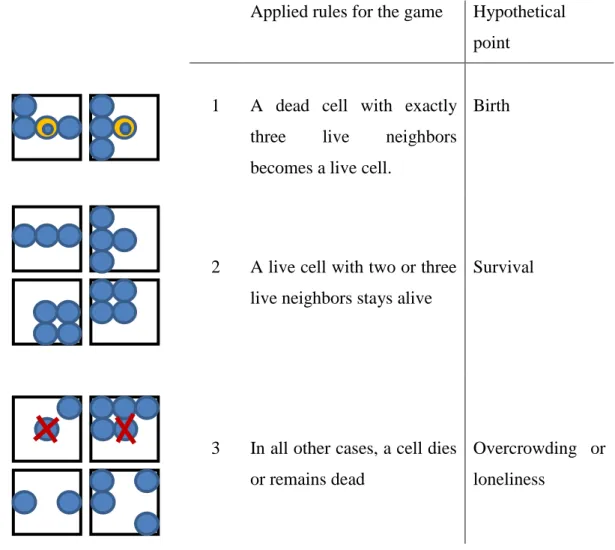
Inspiration to research is Conway’s game which is called “Game of Life”; The game is an example of a cellular automaton and played on an infinite two-dimensional rectangular grid of cells. Each cell can be either alive or dead. The status of each cell changes each turn of the game depending on the statuses of that cell's 8 neighbors. Neighbors of a cell are cells that touch that cell, either horizontal, vertical, or diagonal from that cell. Rules that apply to game:
10
Figure 2.2: Applied Rules for The Game of Life
Applied rules for the game Hypothetical point
1 A dead cell with exactly three live neighbors becomes a live cell.
Birth
2 A live cell with two or three live neighbors stays alive
Survival
3 In all other cases, a cell dies or remains dead
Overcrowding or loneliness
Hepner and Grenander put the use of a game’s feature in research as a core element, which is there is no self-generated behavior of the cells, and their future movement or direction are entirely a function of each cell’s response to adjacent neighbours.
The model proposed by the Hepner and Grenander driven by a Poisson process with the accordance of random variables equation.
11
And where ui(t) = xi(t), yi(t) shows the location of bird at number i at time t also consecutive functions that part of the equation are:
Fhome, which express the tendency towards the central mechanism, Fvel, which controls the velocity of an individual,
Finteract, which measures the influence of one individual on another P(t), Poisson stochastic process.
involved in the process of simulation. These terms; Fhome, Fvel, Finteract are deterministic and P(t) is intended to simulate the effect of local disturbances. With adding this non-Newtonian term, it clusters the simulation in a way of probability feature.
In the lack of mathematical identification, Reynolds’ simulation (1987) suggests the idea of each boid or bird attempts to reach the velocity of neighbouring boid so that catching the convergence to a mean velocity nearly impossible to observe. In contrast, Hepner and Grenander proposes that each individual is in an attempt to return to preset personal velocity and attracted to a roost.
Although, Heppner and Grenander describe the research as a “trial-and-error”, it gives a sight about flocking, which is the main result from attractiveness between birds’ flight. And also the primary reason why the study is cornestoned is that they prove the Newtonian gravitation force fails to produce flock-like behavior. The other perception that they encounter is why Poisson-based force success when Gaussian fails to represent the behavior of attractive bird.
Before go into deeper swarm theory, optimization topic needs to be represented. In regard to subject, demonstration of a Traveling Salesman Problem (TSP) is used. For a brief guideline, TSP consists of a salesman and a set of cities. The salesman has to visit each one of the cities starting from a certain one and returning to the same city. The challenge of the problem is that the traveling salesman wants to minimize the total length of the trip.
12
Despite an intensive study by mathematicians, computer scientists, and others, it remains an open question whether or not an efficient general solution method exists. Throughout the years, many researches have conceived the algorithms to obtain an optimum solution. As an exemplification, some of the heuristic algorithms are:
Nearest Neighbour, also it is called Greedy algorithm time to time. Initialize with the hometown city. Then the algorithm calculates all the distances to other n-1 cities. Goes to the next closest city. And process continues until all the cities are visited once and only once then back to hometown. Algorithm’s simplicity is the biggest advantage to a solution, however, when the sample size or number of cities are high, it is impractical to make a solution in the terms of time usage. As an example with number of 5 cities, number of tours that need to be complete all possible answers are 12 ((n-1)!/2). When the number of cities increased with an one single city, the total tours rise to 60. With 9 cities it is 20.160, with 81 cities it is 2.899E+120.
Genetic Algorithm is the other best-known approaches to solve TSP problems with the application of evolutionary algorithms. These algorithms are generally based on naturally occurring phenomena in nature, which are used to model computer algorithms. Alongside the Ant Colony Optimization and Artificial Immune System approaches, Genetic Algorithm is the best well-known way of solution.
For a brief explanation, Genetic Algorithm is a type of local search algorithm that mimics evolution by taking a population of strings which encode possible solutions also called individuals and combine them based on a fitness function to produce individuals that are closer to solution. Steps that are constructed sequentially:
13 • Random generation of a population.
• Calculation of each solutions’ fitness.
• Selection of parent strings based on fitness.
• Generating a new string with crossover and mutation until a new population has been created
• Repeating the step 2 and 5 until satisfying solution is reached.
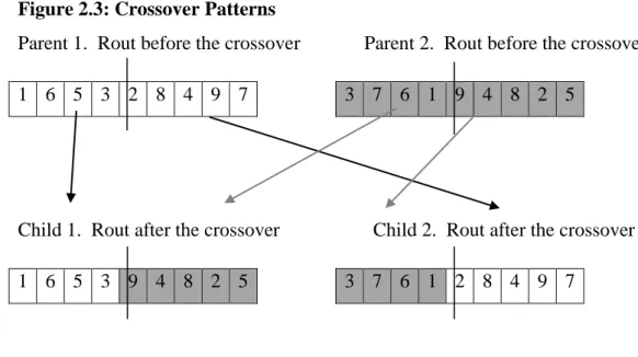
As an illustration to crossover, assume there are 9 (1,2,3,4,5,6,7,8,9) cities in hypothetical country to visit for a salesman, first tour is covered by the rout of 1 – 6 – 5 – 3 – 2 – 8 – 4 – 9 – 7 , and the second one is visited by 3 – 6 – 1 – 9 – 4 – 8 – 2 – 5. Here the first 2 tours are parent strings and then its possible crossovered routs:
Figure 2.3: Crossover Patterns
Parent 1. Rout before the crossover Parent 2. Rout before the crossover 1 6 5 3 2 8 4 9 7 3 7 6 1 9 4 8 2 5
Child 1. Rout after the crossover Child 2. Rout after the crossover 1 6 5 3 9 4 8 2 5 3 7 6 1 2 8 4 9 7
14
Simple swap of parts between two parent tour produces new illegal route which contains stochastic duplicates and its drawbacks come with it that it is possible to visit some cities twice or more while others may not be visited at all
As an example for mutation, main two types of mutation operators: The reciprocal exchange operator simply exchanges two randomly selected cities in rout.
Figure 2.4: Mutation Pattern
And the other operator for mutation, inversion operator selects two random points along the route string and reverses the order of the cities between these points.
Figure 2.5: Inversion Pattern
Neural Networks can be used in TSP optimization other than the Greedy and Genetic based solution. Gelenbe, Koubi and Pekergin (1993) suggests Neural Network based solution to combinatorial optimization problem.
Proposition from the research is comparing the results from The Dynamic Random Neural Network (DRNN) approach which considers the probability leg
15
for a new way to a solution. In DRNN study, they find the optimum solution in %73 of the instances via 10 cities.
The path that evolves the DRNN is “Neural Computation of Decisions in Optimization Problems” by Hopfield and Tank (1985) which is introduced to field as a rapid solution to optimization in that time. Study utilizes the notion of energy function to observe the unionization of the network.
Kennedy (a social psychologist) and Eberhart (an electrical engineer) (1995) propound an epochal idea on swarm intelligence. Research is influenced by Heppner and Grenander’s work (1990). Particle Swarm Optimization is a concept for the optimization of continuous nonlinear functions using particle swarm methodology.
For a broader frame, in PSO, number of simple particles are implemented to search space of some problem and each particle evaluates the objective function at its current location. On contrary to Heppner and Grenander’s bird flock, particles have no mas or volume. And then each particle determines its movement through search space by combining some aspect of the memory of its individual current and best locations with those of other members of the swarm. Each iteration initializes and finalizes with the all particles sequentially. Consequently, swarm as a whole is expected to move close to optimum of the fitness function.
Kennedy and Eberhart adapt the “swarm” term as in used Milonas’s (1994) research, which is constructed by five principles:
• Proximity principle: The population should be able to carry out simple space and time computations.
• Quality principle: The population should be able to respond to quality factors in the environment.
16
• Principle of diverse response: The population should not commit its activities along excessively narrow channels.
• Principle of stability: The population should not change its mode of behavior every time the environment changes.
• Principle of adaptability: The population must be able to change behavior mode when it’s worth the computational price.
Monumental difference between Kennedy and Eberhart’s work from its precursors is their proposal on to abstractness. Previous researches on to bird flocks capture the idea of their adjustment to physical movement such as avoiding predators, optimize temperature. However, Kennedy and Eberhart suggest human adjusts not only physical movement but cognitive or experimental variables as well. Also, study sides people tend to adjust their beliefs and attitudes to their social peers.
Another important point from the study, it reveals the collison subject in the swarm intelligence level accordance to difference physical and non-physical. In cognitive surface, more than one individual can hold exact the same belief without collision, however, two birds cannot occupy the same position in search space.
From nearest neighbor study, as in which population of birds initialized with a position combined by X and Y in two-dimensional space and at each iteration the bird’s (which they call agents) X and Y velocities updated to nearest birds, is with a time passes flock’s direction becomes unchanging. Hence a stochastic variable “craziness” implemented by Kennedy and Eberhart into work which adds some changes to randomly chosen X and Y velocities.
As an assistive sight, they point out that in Heppner and Grenander’s simulation,birds’ movement in an accordance to roost and knows where to land. The objection from Kennedy and Eberhart is the knowledge that somehow implemented their memory before execution of simulation. For example, how can
17
they know where the food was before it put there so that It is a designated place to be landed.
Although, craziness adjustment to simulation seems reasonable at first, Kennedy and Eberhart finds the algorithm works fine in two-dimensional space without of it so that it is removed in the original PSO.
The other implementation from the work, “comfield vector” which is a two-dimensional vector on the XY coordinates to find its absolute position. Each agent is coded to evaluate its current position systematically from this equation:
From the logic of it, at the (100,100) position, the value is 0.
Each agent has a memory of the best value or in other words it remembers the XY position which had resulted in that value. The value is called pbest and the position is pbestx and pbesty. Each agent moves through the space and evaluates the position at the same time. Hence, its X and Y velocities are adjusted. As an example, if it is positioned right of its pbestx, then its X velocity(vx) is adjusted negatively by a random amount weighted by a parameter of the system: vx = vx –
rand*p_increment. Similarly, Y velocities vy are adjusted up and down,
depending on the position of pbesty.
Moreover, each agent continuously has the knowledge of global best position that any member of the flock has found. The variable assigned for the global knowledge free to all members is gbest which is composed of the gbestx and gbesty. And each member’s vx and vy are adjusted from these parameters:
18
Theoretically, pbest has a resemblance to autobiographical memory and each agent holds its own experience throughout out the sequent iteration which has a power to adjust it (if presentx or presenty > pbestx or pbesty, respectively). Following velocity adjustment, after the present situation which is not satisfied as in the past called “simple nostalgia”. The other variable gbest is conceptually analogous to “publicized knowledge” which each individual has a clear recognition to it.
After the agents’ memory presentation which is constructed by their own historical experiment and cumulative global knowledge that is distributed every agent freely, Kennedy and Eberhart’s research aims to transform the 2-dimensional search space into a multi2-dimensional space. In order to capture the social behaviour modelling, more than 2 dimensions is needed (X and Y) while doing that changing presentx and presenty alongside the vx and vy to D x N matrices is used, where D is any number of dimensions and N is the number of agents.
After the conversion of dimensions, some adjustments are applied to algorithm due to review.
• Instead of testing the sign of inequality simply, for instance, if presentx > bestx then the velocity is adjusted into a lower level or if presentx < bestx velocity is adjusted to higher level vice versa, velocities are adjusted according to their difference from best location.
19
• With a realization of no possible way to guess which increment (p_increment or g_increment) should be larger, these terms are substracted from the
algorithm. Also, stochastic factor is doubled to catch a mean of 1 which gives an agent to overfly the target about half of the time.
.
Eberhart’s (1998) research supplies an advancement to original PSO by interpolated the “inertia” term into a first main algorithm.
From the main equation, which is connotated in a simplistic manner above, that is proposed by the Kennedy and Eberhart before three legs contribute to algorithm. First leg is the previous velocity of the agent, following second and thirds are the ones which contributes the change of velocity. In the absence of these firs two legs, agent continues its fly with the same direction and speed. The other point, without a first leg velocity is calculated by only its current and historical positions.
Study suggests without a recognition of previous velocity into algorithm, search for PSO is a process where the search space statistically shrinks through the generations. Hence, the optimization is focused entirely on the local search when the existence of earlier velocity is not viable. However, adding first leg into equation gives agent a tendency to widen its local search space into a global search space and test the new areas. Combining the search for a local and global,
20
an agent optimizes the best. Eventually, research concludes an idea of trade-off between local and global search. Hence, different balances can occur between for searches to implement it, inertia weight “w” is defined into an equation.
Weight of inertia can be positive constant or linear, non-linear function of time.
With a new parameter into a PSO, new paradigm of interaction between global and local search interaction is visualized. From the simulations are performed, between the range of (0.9, 1.2) inertia weights are best suited for the finding a global best.
Eberhart (2000) compares inertia weights and constriction factors in PSO, the constriction factor is included into an algorithm by Clerc (1999). And it suggests a new idea on implementation for a convergence matter, which can be defined as “rehope” method and it re-initializes the agents’ or swarm’s position. In order to emphasize the rudimentary memory of agents. Constriction coefficient suggested by Clerc is:
And new derived formula for the velocity and position with the constriction coefficient is:
21
Traditionally, there are five main non-linear functions to compare inertia and constriction factor. Occasionally, these functions are tested by 30 dimensions at every simulation. As a brief idea on to functions. Equations for these functions are:
Table 2.1: Functions Applied to Comparison
Sphere function:
Rosenbrock function:
Generalized Rastrigrin function:
Generalized Griewank function:
And the results from the comparison are sided to constriction factor is better approach than the inertia weight approach. Particularly, constriction approach’s outcomes are constituted with a faster result and a higher average quotient for
22
Sphere, Rosenbrock and Schaffer’s f6 function. Also for the generalized Rastrigrin function, result is ambiguous to choose an approach. Only function that backs the inertia weight approach is Generalized Griewank function yet it is yielded less quickly to desired error value 85 percent of the time. Moreover, with limiting the search space impressing outcomes are concluded when the Vmax is conditioned to be Xmax (Vmax = Xmax).
Clerc and Kennedy (2002) enhances the main PSO with an objection to original one which contains random weighting extension to control parameters. With adding an arbitrary weighting term to equation, algorithm has tendency to explode or become a “drunkard’s walk”.
Main source of that explosion is caused by the limitation of velocity. With an implementation of Vmax makes algorithm open to an overshooting the search space. To avoid the explosion, research introduces a new constriction coefficient that can prevent the problem and also these coefficients have an auxiliary effect on particles to converge on local optimum.
Trelea’s (2002) research has an impact on parameter selection. From previous researches, Trelea states that selection of the algorithm parameters is empirical to a large extent which population parameter is chosen between the range of 20-50, generally.
The other advantageous topic which is mentioned in the work is to give a clear identification to legs which are constructed the equation jointly. Cognitive local search is generalized as an Exploration and the social component for a search to global optimum is symbolized as an Exploitation. Also, study suggests some parameters that are established before gives no flexibility to algorithm which is why some of them are needs to be substracted from the equation without a loss of generality.
23
2.2. Overview of PSO
Poli, Kennedy and Blackwell (2007) gives a clear and sophisticated summary to Particle Swarm Optimization’s evolvement for the period from the day one which is first discovered in 1995 through to 2007.
As an original PSO process here is the practical PSO scheme Kennedy and Eberhart applies first:
Figure 2.6: Original PSO Scheme
• Initialization process is started by implementing the particles with random positions and velocities on D dimensions in the search space.
24
• Evaluation process interpreted in the D dimensions search space. • In the evaluation phase, if present value is better than pbest, pbest is
needed to be set equally to present value. Also, the new position by the present value of particle is needed to be reset as a new best location. • After the identifying and assignment of best particle, changing the velocity
and its position is applied by the equation below:
• Each component of velocity is between the range of [ -Vmax, +Vmax].
Even though, search space is usually interpreted as a 3 or more-dimensional infinite space, on contrary, study simulates the historical cognitive leg (U (0, φ1) ⊗ (p − x)) and social exploitation leg (U (0, φ2) ⊗ (pg − _x)) as a force to accompanies with Newton’s second law. Also, φ1/2 and φ2/2 represent the mean rigidity. Hence, by changing φ1 and φ2, simulation can be more or less responsive. To limit the sensibility of legs, implementation of −Vmax, +Vmax is seemed to be affective in the early phase of the PSO algorithm.
After the inertia weight connotation, research sides the idea of appointment of appropriate inertia weight “ω” and acceleration coefficients “φ1” and “φ2” makes the algorithm much more stable. Also, it seems with implementation of Vmax or adding balanced weights and coefficients indifferent.
Constriction implementation into an equation follows the inertia narration, when PSO is simulated without a limitation to velocity, reaching an unacceptable level in few iterations is a consequential affect if it. Within a simplest algorithm which is included as constriction parameter, and acceleration coefficients are ranged between 0 to 4, PSO overcomes the problems which is not suitable for the PSO with inertia weights.
25
2.3. Topology in PSO
In standard and developed PSOs, success from the particle is constituted by the previous best success from its own or from “some other particle”. As a description, some other particle is usually defined by the gbest and lbest. As in gbest population, each individual particle is influenced by the information which is gathered from each particle cumulatively. On the lbest, information is gathered from the adjacent particles accordingly to topology of the swarm. Eventually this information from the lbest can be visualized as in single figure below: (like a ring for a lbest)
Figure 2.7: Ring Topology
Kennedy and Mendes (2002) transforms the idea of lbest into fully informed particles which each individual can influenced by all the other particle instead of just two particle that is located nears them. This other consideration is implemented into an equation as below
The equation is altered the lbest topology into a fully connected particle swarm. However, the disadvantage of fully informed particles, best successes may be
26
skipped time to time. Fully informed particles can be visualized as in figure below.
Figure 2.8: Fully Informed Particle Topology
Therefore, in the process of simulation, topology framing is a major explanatory force behind individuals’ success for in the search space. Also, it gives a clear identification to individuals social behavior, whose local and particular interactions between them are decisive to algorithm.
Medina, Pulido and Torres (2009) compares the main topologies which are used in the process of implementing an algorithm. Also, these topologies impact the social connections between the particles to find a better solution in the search space.
Ring topology
Also, it can be named lbest version from the standard PSO, the individuals are only affected by the two adjacent neigbours. (From the figure of 2.7). Hence, there is a possibility that one individual can converge to a local optimum while the other particle approaches the smaller local optimum at the same time or remains searching. Main idea however, each particle gradually reaches the optima by the aid from the swarm.
27
Fully Connected Topology
Each particle is connected to other all remaining particle. (From the figure of 2.8). It can be reframed as gbest version. In this topology, each particles direction is constructed by the global best and each particle moves through the gbest orientationally.
From the researches, population that are constituted by the gbest or fully connected particles is tend to converge more rapidly than lbest or ring style toplogy to an optimum. However, searching for a local optimum seems to be more susceptible than local best approach.
Star Topology
Star topology is constituted by a central particle which influences all the remaining particles also it can be influenced by all other members vice versa. Main inside from the star topology is how individual reacts when the information is gathered by the main individual and that main individual is the only influencer to a search for the swarm direction.
Influencer takes a role as a central particle to direct a flight. While choosing a destination, the primary force behind the destination decision is compering the information from the attached particles to itself. This central particle evaluates all the information from the population.
Main advantageous from the star topology is that can prevent premature convergence to a local optimum, at the same time it can limit the population’s collaboration ability. Star topology can be visualized as in figure below.
28
Mesh Topology
In mesh topology, each particle in the middle of the mesh is connected to four neigbours which is located to its south, north, east and west. The particles that are positioned to be in the boundary of the mesh has three connected particles.
Main disadvantage of asset which is constructed by the mesh topology, it allows the particles to overlap. Hence, it can be possible to allow redundancy in the algorithm. Mesh topology can be visualized as in figure below.
Figure 2.10: Mesh Topology
Toroidal Topology
Toroidal topology can be seen as advancement to a mesh topology in the face of the particle’s connection to each other. Plus, to mesh topology, each particle has four adjacent particles even they are located to boundary. Toroidal topology can be visualized as in figure below.
Figure 2.11: Toroidal Topology
Tree Topology
As in the star topology, tree topology again constructed by the central particle. But, in this one particles organized by the hierarchical order. Sequential particles
29
to central one has one level lower hierarchic power in the information gathering surface.
Central particles act as a mother in the search for a best solution. She gathers the information from the children and choose the destination accordingly to it. Tree topology can be visualized as in figure below.
Figure 2.12: Tree Topology
2.4. PSO on Finance
Primary focus on the finance through the PSO is portfolio construction. With the implementation of mean-variance model for portfolio, finding an appropriate algorithm to a Markowitz’s efficient frontier has been a hot topic for researchers. As a detection to selection surface, Nenortaite and Simutis (2005), Nenortaite (2007) implements a decision-making model into algorithms. Portfolios can be constituted other than stocks, Reid, Malan and Engelbrecht (2014) creates a currency portfolio under the carry trade model. Also in the real world, portfolios are constructed under the several constraints. As a solution to that problem, evolutionary algorithms such as birds flying algorithm by Meybodi, Denavi and Sadeghian (2015), Ayodele and Charles (2015) are used in the 21th.
Moreover, as a perception to Turkish stock market and a different approach which is computerized solution to portfolio selection problem, Kara, Boyacioglu and Baykan (2011), Boyacioglu and Avci (2010) proposed particular researches.
30
Cura (2008) compares the Generic Algorithm, Particle Swarm Optimization and Tabu Search to trace its efficient frontier. From the study, in an attempt to construct a low risk portfolio, PSO is resulted in better outcomes.
2.5. Applications of PSO
One of the main attractiveness of PSO derives from its simplicity. Also, its features that has a resemblance to Artificial Intelligence makes it preferred approach to optimization problems.
31
CHAPTER 3
DATA AND METHODOLOGY
For the experimental study, monthly data is gathered from finance. Yahoo. Data is consisting of six stock which are participated in Bist 30 Index (XU030). Stocks are Turkiye Petrol Rafinerileri A.S. (TUPRS), Turk Hava Yollari A.O. (THYAO), Otokar Otomotive ve Savunma Sanayi A.S. (OTKAR). Koza Altin Isletmeleri A.S. (KOZAL), Turkiye Garanti Bankasi A.S. (GARAN) and Arcelik A.S. (ARCLK).
Stocks are examined by their monthly return. However, Recent changes in the Yahoo’s application programing interface caused data to be reviewed in the Microsoft Office Excel and then to fetch into MATLAB.
Stocks’ monthly returns and close prices are analyzed between the period of December 31st 2010 to December 30th 2015 and monthly return calculation is formulated as:
Where, P(t) is the closing price, P(t-1) is the closing price in the day before and M(t) is the monthly return.
32
Graph 3.1: TUPRS, OTKAR and KOZAL’S Monthly Prices
33
Graph 3.3: THYAO, GARAN and ARCLK’S Monthly Prices
Graph 3.4: THYAO, GARAN and ARCLK’S Monthly Returns
Between December 2010 and December 2015 BIST30 is showed gradual increase and decrease monthly.
34
Graph 3.5: BIST 30 Index
The main reason for using monthly return is dividends’ withholding tax, in the range of the period which data is evaluated, benefits from stocks other than a capital gain are faced deduction at source. And the day before and after the dividend payment, closing prices are open to be affected by the arbitrary adjustment. The other inefficacious parameter that can influence the asset price in a trivial way is stock splits.
As a description, other auxiliary definitions which are implemented to simulation, occasionally:
Mean
A mean is the simple mathematical average of a set of two or more numbers. It is formulated as:
35 Variance
Variance, or risk, is a measure of the volatility or the dispersion of returns. Variance is measured as the average squared deviation from the mean. Higher variance suggests less predictable returns and therefore a riskier investment. The variance (σ2) of asset returns is given by the following equation.
where Rat is the return for period t, T is the total number of periods, and μ is the mean of T returns, assuming T is the population of returns.
Standard Deviation
The standard deviation of returns of an asset is the square root of the variance of returns. The population standard deviation (σ) and the sample standard deviation (s) are given below. The variance can be seen as amount of difference between the data and to their mean. To find the standard deviation, square root of variance is taken. As an illustration, standard deviation is formulated as below:
Where, X is a single variable, N total number of variable and µ is the mean.
Coefficient of Variation
Covariance can be seen as a movement of the co-movement in linear association between two random variables.
36
Where, 𝞼 is the standard deviation of returns and r is the return.
In construction the experimental portfolio by particle swarm optimization, first, traditional selection on instruments to constitute a portfolio is demonstrated. Then, outputs are compared with the PSO approach. In traditional way, ‘mean-variance’ portfolio is used.
Mean-Variance Analysis
It is a process of weighing risk, variance in that implementation, against expected return. The reason behind the practice is to give investors a more suitable and efficient investment choices. In doing that, bottom line is seeking a lowest variance for a given expected return or seeking the highest expected return for a given variance vice versa.
Mean-Variance portfolio is represented the fundamental implementation of ‘modern portfolio theory’ and it is a representation of the optimal allocation of assets between risky and risk-free assets.
Modern Portfolio Theory (MPT)
MPT is a theory on how ‘risk-averse’ investors can construct portfolios to maximize or optimize expected return based on a given level of ‘market risk’. If an investor chooses the guaranteed outcome, he/she is said to be risk averse because the investor does not want to take the chance of not getting anything at all. Also, theory suggests there is a constructed line that illustrates investors the best possible return they can expect from their portfolio, given the level of risk that they are willing to accept.
37
Figure 3.1: Return and Risk Relation
Risk-averse
Risk aversion can be seen as the degree of an investor’s inability and unwillingness to take risk. In general, investors are likely to shy away from risky investments for a lower, but guaranteed return. If an investor chooses the guaranteed outcome, he/she is said to be risk averse because the investor does not want to take the chance of not getting anything at all. Generally, they look for a ‘safer’ investment as in Government Bonds.
Market Risk
It is the possibility for an asset to experience losses due to factors that affect the whole performance of the financial markets. It can also be called systematic risk which is opposite of idiosyncratic risk that cannot be eliminated through diversification. One of the main systematic risk is changes in interest rate.
38 Sharpe Ratio
The Sharpe ratio is used to compare the portfolio return in excess of a riskless rate with the volatility of the portfolio return. The ratio provides a measure of how much the investor is receiving in excess of a riskless rate for assuming the risk of the portfolio. The Sharpe ratio is calculated for any portfolio with using the formula below.
Where, rp is expected portfolio return, rf is risk free asset’s return and 𝞼 is the portfolio.
Modern Portfolio Theory addresses the issue that implementing a new asset to a diversified portfolio which has a correlation of less than one with the basket of portfolio can diminish the portfolio risk without sacrificing the return. Adding such asset to portfolio will rise the Sharpe ratio of portfolio.
Risk-Free Rate
The risk-free rate of return is the hypothetical rate of return of an investment without a risk. The risk-free rate demonstrates the additional return which an investor would expect from a riskless investment over a specified period of time.
In simulation risk-free rate is represented as 0.09 % annually. It is average to annual Rf from 10-year Turkish Government Bond.
Capital Allocation Line
A graph line that describes the combinations of expected return and standard deviation of return available to an investor from combining the optimal portfolio
39 of risky assets with the risk-free asset.
Value at Risk
In its most general form, A money measure of the minimum value of losses expected during a specified time period at a given level of probability. For example, a financial firm may determine an asset has a 4% one-month VaR of 3%, representing a 4% chance of the asset decreasing in value by 3% during the one-month time period.
Conditional Value at Risk
It is a risk assessment technique which is used to reduce the probability that a portfolio will incur large losses. This is performed by assessing the likelihood specific confidence level which a specific loss will exceed the value at risk. Mathematically speaking, CVaR is derived by taking a weighted average between the value at risk and losses exceeding the value at risk.
Mean Absolute Deviation
Likewise the standard deviation it takes the difference between each observed value and the mean, which is the deviation. Then, uses the absolute value of each deviation, adding all deviations together. Lastly, divides by n, the number of observations. It can be formulated as below:
40 Semivariance
Semivariance is a measure of the dispersion of all observations that fall below the mean or target value of a data set. With a determination of two bounds, which are lower and upper, it can be calculated as below.
41
CHAPTER 4
IMPLEMENTATION OF MEAN-VARIANCE PORTFOLIO
Mean-variance portfolio implementation starts with importing the data from desktop and subtraction of symbols sequentially. Then, stocks monthly return calculation and defining of portfolio,
Figure 4.1: Code of Data Implementation in Mean-Variance Portfolio
T = readtable('priceslast.xlsx');
symbol = T.Properties.VariableNames(1:end); dailyReturn = tick2ret(T{:, 1:end});
p = Portfolio('AssetList', symbol, 'RiskFreeRate', 0.09/12);
And estimation of Asset Moments with portfolio constraints follows.
Figure 4.2: Code of Asset Moments and Portfolio Constraints
p = estimateAssetMoments(p, dailyReturn); p = setDefaultConstraints(p);
Main constraint is total weights from stocks should be equal to 1 in the range of 0 to 1.
Figure 4.3: Code of Comparison to Sharpe Ratio
w1 = estimateMaxSharpeRatio(p);
Before the last part of screening the risk and return accordance, weights are determined.
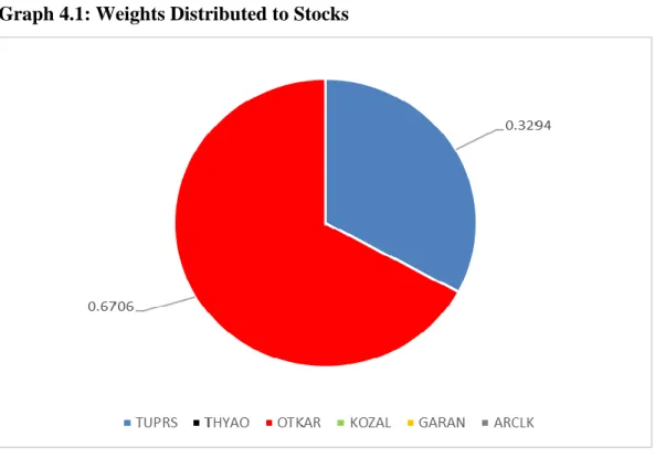
Weights are distributed to stocks from solution: TUPRS – 0.3294, THYAO – 0, OTKAR – 0.6706, KOZAL – 0, GARAN – 0, ARCLK – 0.
42
Graph 4.1: Weights Distributed to Stocks
To conclude and assign the risk and return, portfolio moments are implemented accordingly to portfolio and weights.
Figure 4.4: Code of Risk and Return
[risk1, ret1] = estimatePortMoments(p, w1)
The results for risk and return are 0.0924 and 0.0269, respectively.
With the implementation of figure code, efficient frontier and optimal portfolio point in the terms of risk and return relationship is visualized.
43
Graph 4.2: Efficient Frontier of Mean-Variance Portfolio
From the monitoring of visualization, worst performance is conducted by KOZAL and even tough GARAN shows some decent performance in the terms of risk measurement, still, it is way far away from the optimal return that constructed by the program.
ARCLK and THYAO have modest performance through the period, yet, outputs that they display are not near the optimal portfolio.
TUPRS and OTKAR are the only two participants that take a role in the fitted portfolio. In terms of the return leg, OTKAR shows a remarkable performance. Also, TUPRS’s variance accordingly to risk measurement is the primary reason why it takes nearly one third of the weight in the portfolio.
44 3 Stock Simulation
Another experiment is applied to OTKAR, TUPRS and KOZAL as if they are the only investment basket that can be choiced. In the simulation, stocks’ expected monthly returns and their covariance are the auxiliary force behind the asset allocation.
The expected monthly returns for stocks OTKAR, TUPRS and KOZAL’s are 0.0166 0.0320 and 0.0050. In the program, main answer for algorithm to solve is what if constraints are limited to just gathering weights are equal to 1.
The other implemented variable is risk-aversion limitation which is ranged 0.01 to 3 per cent. With risk-free asset 0.75 % monthly adding and expected returns from OTKAR, TUPRS and KOZAL, which is calculated as mean monthly return through the examined period. Capital Allocation Line:
45
CHAPTER 5
IMPLEMENTATION OF PSO PORTFOLIO
Implementation of particle swarm optimization is constructed by the sections of problem definition, parameter interpretation, initialization, main loop, and results.
Problem definition
In this section, interpretation of problem which will be solved by the PSO is implemented, the main component of the solution is cost function which program focused to minimize its value.
After the cost function, search space is implemented. It is part of the program as numerator of the decision or unknown variables.
Figure 5.1: Code of Cost Function and Population limits
CostFunction=@(x) PortCost(x,model); nVar=size(model.R,2); VarSize=[1 nVar]; VarMin=0; VarMax=1;
Also, particle is a vector who searches a solution in matrice so that any position is a vector and has a size of one row and nVar columns. Lastly, the range of the decisions are implemented as lower and upper bound.
PSO parameters
In parameter section, code is started with the maximum iteration that PSO applies, then swarm size is implemented.
46
In the study, Particle Swarm Optimization with Constriction Coefficient approach is used so that inertia weight W, cognitive term which is an individual acceleration coefficient C1 and social acceleration coefficients are in the presents of constriction coefficient. Lastly, velocity limits for each particle is introduced. Damping of inertia weight is not used.
Figure 5.2: Code of Main Approach and Limits
MaxIt=100; nPop=40; chi=2/(phi-2+sqrt(phi^2-4*phi)); w=chi; wdamp=1; c1=chi*phi1; c2=chi*phi2; VelMax=0.1*(VarMax-VarMin); VelMin=-VelMax; Initialization phase
Any initialization of the event such as particle position, local best or global best starts in this phase. To store the experience as an individual and as a swarm templates are constructed. The store is gathered by the position, cost, out and velocity fields and their best values which are experienced before. Also repetition for the whole swarm is written.
Figure 5.3: Code of Particle Initialization
empty_particle.Position=[]; empty_particle.Cost=[]; empty_particle.Out=[]; empty_particle.Velocity=[]; empty_particle.Best.Position=[]; empty_particle.Best.Cost=[]; empty_particle.Best.Out=[]; particle=repmat(empty_particle,nPop,1); BestSol.Cost=inf;
47
In the for loop, create and set the random particles by uniformly distributed data is followed. Then velocity initialization, evaluation of the particle and updating the local and global best are implemented. Also, comparison of local and global bests is interpreted. Finally, array to catch the best solution in each iteration is written.
Figure 5.4: Code of Velocity Initialization and Catcher
particle(i).Position =unifrnd(VarMin,VarMax,VarSize); particle(i).Velocity=zeros(VarSize); [particle(i).Cost, particle(i).Out] =CostFunction(particle(i).Position); particle(i).Best.Position=particle(i).Position; particle(i).Best.Cost=particle(i).Cost; particle(i).Best.Out=particle(i).Out; particle(i).Best.Cost<BestSol.Cost BestCost=zeros(MaxIt,1); Main loop
After the definition of problem and parameters then the initialization phase, main loop is added to code and it is processed by the for loop to cover the whole iteration. Also, another for loop to interpret each particle.
Firstly, particle i’s velocity is updated for each iteration accordingly to previous value of velocity plus the position factor which is randomly conducted and represents to best position from the local experience minus the current position. Also, same conduction is implemented for the global experience.
Figure 5.5: Code of Updating the Velocity and Position
particle(i).Velocity = w*particle(i).Velocity ... +c1*rand(VarSize).*(particle(i).Best.Position-particle(i).Position);
+c2*rand(VarSize).*(BestSol.Position- particle(i).Position);
For algorithm to converge the variable limits, velocity and position limits are applied. Also, evaluation process is interpreted in this main loop.
48
Figure 5.6: Code of Convergence
particle(i).Velocity = max(particle(i).Velocity,VelMin); particle(i).Velocity = min(particle(i).Velocity,VelMax); particle(i).Position = max(particle(i).Position,VarMin); particle(i).Position = min(particle(i).Position,VarMax); [particle(i).Cost, particle(i).Out] = CostFunction(particle(i).Position);
Lastly, for updating the personal best, comparison is implemented into code. Then, global best update is followed, sequentially. To conclude, again empty array is implemented to catch the best solution in the iterations.
Figure 5.7: Code of Updating the Personal Best and Catcher
particle(i).Cost<particle(i).Best.Cost; particle(i).Best.Position=particle(i).Position; particle(i).Best.Cost=particle(i).Cost; particle(i).Best.Out=particle(i).Out; particle(i).Best.Cost<BestSol.Cost BestSol=particle(i).Best; BestCost(it)=BestSol.Cost;
Figure 5.8: Code of Solution
out.BestSol=BestSol; out.BestCost=BestCost;
Along with the general scheme for the Particle Swarm Optimization, other functions are implemented to MATLAB code in order to detect the portfolio construction.
Main reason behind the PSO interpretation is its utilitarian procedure to observe each solution for the weights implementation on each iteration. Also, each solution for the swarm with population of 15 particles are affected by the elements that are introduced in the function codes. To give a clear perception to each solution, each five solutions to weights from the program is illustrated.