Reflectance-Based Foster
Impedance Data Modeling
Frequenz61 (2007) 7-8
By Metin Şengül
Abstract – A reflectance-based method is presented, to model a set of given Foster impedance data as a lossless, singly terminated two-port consisting of lumped-elements in short or open termination. The basis of the new method rests on the interpolation of the given data as a realizable bounded-real (BR) reflection func-tion. The desired circuit model is obtained by synthesizing this funcfunc-tion. An algorithm to generate the circuit model is presented, and an example is included, which illustrates the utilization of the proposed modeling method.
Index Terms – Circuit optimization, gradient methods, iterative methods, lossless circuits, modeling, passive networks.
1. Introduction
For many communications engineering applications, circuit models for measured data obtained from physical devices or sub-systems are inevitable. Typical examples include the characteri-zation or assessment of front-ends in terms of the minimum noise figure level or the maximum power transfer capability [1], the design of antenna matching networks or microwave amplifi-ers for mobile or wireless communication [2], and the fast simu-lation of high-speed, high-frequency circuits for analog/digital communication systems [3]-[6].
In broadband matching applications, after designing the imped-ance matching network, a Foster part (i.e., that part of the matching network, whose real part of the input impedance is zero) may be needed to improve the matching performance [7]-[8]. In [9], a Foster impedance data modeling method is presented. Briefly, the general form of a Foster function Xf( )ω on the jω -axis can be described as 0 2 2 ( ) 1 n r f r k k X k p r
ω
ω
ω
ω
ω
= ∑ − + ∞ = − . (1) Re D p One can always introduce a pole pr to the Foster form specifiedby (1) that passes through a given point
i . Selecting
( ,ωi Xf) pr
properly in advance, the residues k k and can be computed by solving (1) point by point for the given data set. 0
,
r k∞
In this work, the given Foster impedance data are modeled with-out the need to introduce poles, by lossless lumped-elements which constitute a two-port in short or open termination, with the resulting input reflection coefficient S11( )p (Fig. 1).
Lossless Two-port Lossless Two-port S11(p) S11(p) (a) (b)
Fig. 1: Lossless two-port a) short termination b) open termination. For a lumped-element lossless two-port like the one depicted in Fig. 1, the scattering matrix can be written as [10]:
11 12 21 22 ( ) ( ) 1 ( ) ( ) ( ) ( ) ( ) ( ) ( ) ( ) S p S p h p f p S p S p S p g p f p h p µ µ − = = − − , (2)
where g p h p( ), ( ) and f p( ) are real polynomials in complex frequency p= +σ jω, µ= f(−p) / ( )f p = ±1 is a unimodular constant and g p( )
( ), (
is a strictly Hurwitz polynomial. The three functions g p h p), f p( ) are related by energy conservation, namely, the Feldtkeller equation
( ) ( ) ( ) ( ) ( ) ( )
g p g−p =h p h p− +f p f −p .
In the next section, the properties of singly terminated networks are discussed in line with [11]. Then, after a short review of the gradient method, its application to the modeling problem is dis-cussed. Finally, an algorithm is presented and illustrated in terms of an example.
2. Singly terminated networks
The input impedance of the network seen in Fig. 1 can be written as 11 11 ( ) ( ) 1 ( ) ( ) ( ) 1 ( ) ( ) ( ) ( e o e o N p N p S p N p Z p S p D p D p D p + + = = = − + ), (3)
where N p( ) and D p( ) are the numerator and denominator polynomials of the impedance function; the subcripts “ ” and “ ” refer to the even and odd components, respectively.
e o
The average power absorbed by the two-port network must be zero, since all the elements are lossless and the network is terminated by either an open or a short. In this case, one can write
{
}
2 2 ( ) ( ) ( ) ( ) ( ) 0 ( ) ( ) e e o o e o N p D p N p D p Z p D p − = = + (4a) or ( ) ( ) ( ) ( ) 0 e e o o N p D p −N p D p = , (4b)where Re
{
Z p( )}
represents the real part of the impedance( )
Z p .
Since the even and odd parts of the numerator and denominator cannot be zero simultaneously, either both N pe( ) and D po( )
vanish, leading to ( ) ( ) ( ) o e N p Z p D p = , (5a)
or both N po( ) and D pe( ) are zero, leading to
( ) ( ) ( ) e o N p Z p D p = . (5b)
This leads to the conclusion that the input impedance of a singly terminated network can be described by either a ratio of even-to-odd or odd-to-even polynomials.
Using (3) and (4a), it can be shown that for singly terminated networks S11( )p =1 or, equivalently, S11( )p S11(−p) 1= . From (2) follows, therefore, that
( ) ( ) 1 ( ) ( ) h p h p g p g p − = − . (6)
Assuming that h p( ) does not equal g p( ), which would result in the trivial case where 11=1 at all frequencies, we conclude that
) p S ( g α = − ( ) ( ) h p = ± −g p (7) and 11 ( ) ( ) ( ) ( ) ( ) g p g S p p g p α g p − − = ± = . (8)
At p=0, S11( )p can be either α= +1, corresponding to an open termination, or α= −1, which corresponds to a short termination.
194
This work was supported in part by the Scientific and Technical Research Council of Turkey (TÜBİTAK), Scientific Human Resources Development (BİDEB). This research has been conducted in part within the NEWCOM Network-of-Excellence in Wireless Communications funded through the EC 6th Framework Programme.
Brought to you by | Kadir Has University Authenticated Download Date | 12/6/19 8:45 AM
Frequenz 61 (2007) 7-8 3. Application of gradient method to foster impedance
data modeling
The gradient of a function F at x=( , , ,x x1 2…xN) is defined as
1 2 ( ) ( ) ( ) ( ) , , , N F F F F x x x ∂ ∂ ∂ ∇ = ∂ ∂ ∂ x x x x … , (9) n
where thex ii;
{
=1, 2, ,… N}
constitute the variables of the function.N
The gradient for a multi-variable function is analogous to the de-rivative of a single-variable function in the sense that it can have a relative minimum at only when the gradient at is the zero vector. A standard result from the calculus of multi-variable func-tions states that the direction of steepest decrease of
x x F at is the direction given by −∇ . x ( )x ( )x F
The goal of minimization is, therefore, to reduce ∇ to its minimal value of zero. Given the initial approximation , one chooses F (0) x
(
(1)= (0)− ∇γ F (0) x x x)
(10)for some constant γ >0 )
, which defines the step-size.
Assume S jω is the reflection coefficient data constructed from (
the given Foster impedance data Z jω , and ( ) S11(j )ω is the calcu-lated reflection coefficient of the model. It is desired to have
11( ) S j
( )
S jω = ω at the end of the modeling process. The error between the given and calculated reflection coefficients can accord-ingly be defined as 11 ( ) ( ) ( ) ( ) ( ) ( ) h j j S j S j S j g j ω ε ω ω ω ω ω = − = − . (11a)
The magnitude of the error is 2 (j ) ( j ) (j ) ε ω = −ε ω ε ω ( ) ( ) ( ) ( ) ( ) ( ) h j h j S j S j g j g j ω ω ω ω ω ω − = − − − − . (11b)
To reduce the error until it drops below an acceptable value δ , any iterative method may be employed. If the gradient method is applied, according to (10) and the results of Section II, the values of the numerator polynomial of the reflection coefficient can be calcu-lated as ( ) 2 ( 1) ( ) ( ) 2 ( ) ( ) ( ) ( ) ( ) ( ) ( ) ( ) ( ) i i i i h i i i h j h j j j h j h j ω ω γ ε ω ε ω ω γ ω + = − ∇ ∂ = − ∂ ( ) ( ) ( ) ( ( ) ( ) i i i j h j ) g j ε ω ω γ ω − = + . (12) X = B=α ω
For singly terminated networks, at the end of the iterative process defined above, h j( ω)= ± −g( jω) must be fulfilled. If these values are multiplied by their complex conjugates, g jω is reached, ( )2
which describes an even polynomial in the variable ω such that 2
2 2 4
0 1 2
( ) ( ) ... n n 0 ;
Gω = g jω =G +Gω +Gω + Gω2 〉 ∀ω, (13) where is the desired degree of the polynomial n g p( ) and, at the same time, the number of elements in the model.
The coefficients
{
G G G0, ,1 2,...Gn}
2
can easily be found by any linear or nonlinear interpolation or curve fitting method as described by [9]. Then, replacing ω by −p2, one can extract g p( )
( )
from by explicit factorization. In this step, obvi-ously the roots of are computed, and then,
2 ( ) ( ) G p− =g p g(−p) 2 ( ) G p− g p ) is con-structed on the left half-plane (LHP) roots of as a strictly Hurwitz polynomial.
2
(
G p−
4. Generation of the model Inputs:
• Z j(ωi)= jXf( );ωi i=1,2,..,N : Given Foster impedance data.
• : Desired number of elements in the model.
• α : Termination type, α= −1 for short termination, and
1
α= + for open termination.
• h p( ) : Initial polynomial h p( ). See Step 2 below. • g0 : Constant term of the polynomial g p( ). • γ : Step-size of the Gradient process.
• δ : The stopping criteria of the sum of the square errors. Computational Steps:
Step 1: Calculate reflectance data from the given Foster imped-ance data via ( ) ( ) 1
( ) 1 Z j S j Z j ω ω ω − = + .
Step 2: A proper initial polynomial can be obtained by the following procedure: From (8) follows that
( ) h p ( ) ( ) ( ) g −p =αS p g p . Expressing 2 0 1 2 ( ) n n
g p =g +pg +p g + +… p g , we arrive at the following equation: 2 0 1 2 2 0 1 2 ( 1) ( ) n n n n n g pg p g p g S p g pg p g p g α − + − + − = + + + + … … (14)
If the coefficient g0 is selected as a user-defined coefficient, and p= jω is substituted into (14), the following set of linear equations is obtained: A X =B, (15) where 2 1 1 1 1 2 2 2 2 2 2 1 1 1 1 2 2 1 (1 ( )) (1 ( )) (1 ( )) (1 ( )) (1 ( )) (1 ( )) ( 1) ( ) (1 ( 1) ( )) ( 1) ( ) (1 ( 1) ( )) ( 1) ( ) (1 ( 1) ( )) N N N N n n n n n n n n n N N j S j S j j S j S j A j S j S j j S j j S j j S j ω α ω ω α ω ω α ω ω α ω ω α ω ω α ω ω α ω ω α ω ω α ω + + + − + − − − + − − = − + − − − + − − + − − + − 1 2 n g g g and 1 0 2 0 0 ( ) ( ) ( N) S j g S j g S j g α ω α ω − − − .
After solving (15), the polynomial g p( ) is obtained, and the initial polynomial can be formed subsequently according to (7). The
( )
h p 0
g -value can be supplied by ad-hoc choice. Step 3: Form 11 ( ) ( ) ( ) g p S p g p α − = .
Step 4: Calculate the sum of the square error via 11 (j ) S j( ) S (j ) ε ω = ω − ω and 2 ( ) c j δ =
∑
ε ω . δ ≤δ Step 5: If c , synthesize 11( ) ( ) ( ) g p S p g p α − = and stop. Otherwise, go to the next step.Step 6: Calculate ( ) ( ) ( ( ) ) j h j h j g j ε ω ω ω γ ω −
= + over the sample frequencies.
Step 7: Calculate G(ω2)=g(jω) (g −jω , and form )
( ) ( )
g p h p
α − = .
195
Step 8: Go to Step 3.Brought to you by | Kadir Has University Authenticated Download Date | 12/6/19 8:45 AM
Frequenz 61 (2007) 7-8
5. Example
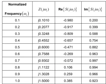
In this section, an example is presented, to illustrate the imple-mentation of the proposed method. The imaginary part of an impedance consisting of an inductor in series with the parallel combination of a capacitor and a resistor, with the normalized values: L=1, C=2, R=1, was used to construct the Foster imped-ance. The Foster impedance and the real and imaginary parts of the reflection coefficient data (see (3)) are listed in Table I.
Table 1: Calculated Foster impedance and reflection coefficient data.
Normalized Frequency
( )
ωi ( i) Z jω Re{
S jω( i)}
Im{
S jω( i)}
0.1 j0.1010 -0.980 0.200 0.2 j0.2077 -0.917 0.399 0.3 j0.3248 -0.809 0.588 0.4 j0.4552 -0.657 0.754 0.5 j0.6000 -0.471 0.882 0.6 j0.7588 -0.269 0.963 0.7 j0.9302 -0.072 0.997 0.8 j1.1122 0.106 0.994 0.9 j1.3028 0.259 0.966 1.0 j1.5000 0.385 0.923In the next step, short termination (α= −1 ( )
), and four elements ( ) were selected for the model. Applying the proposed algorithm, the polynomials h p and
4 n= ( ) g p were determined as 2 3 ( ) ( ) 1.2491 1.3141 0.4426 0.0470 0.0125 h p g p 4 p p p = − − = − + − + − p 4 and 2 3 ( ) 1.2491 1.3141 0.4426 0.0470 0.0125 . g p = + p+ p + p + p The
synthesis of the obtained impedance function 11 11 1 ( 1 ( S p S p ) ) ( ) Z p = + −
resulted in the equivalent circuit depicted in Fig. 2.
L1 L2
C1
C
2) ( p Z
Fig. 2: Obtained model of the Foster impedance data given in Table 1. C1=0.26596, C2=0.13621, L1=0.5048, L2=0.54723.
A comparison of the original and re-constructed impedance values is illustrated by Fig. 3.
Fig. 3: Comparison between the given and model impedances.
The error between the given and model impedances seen in Fig. 3 can be further reduced, if the number of elements in the model is increased. But in this case, dissipation losses will increase, since the components are lossy in practice. Therefore, it is usually preferred to use the least number of elements in the Foster models.
6. Conclusion
A reflectance-based technique was presented to model measured or computed Foster impedance data. Unlike other available tech-niques, the proposed method does not require to introduce any pole. The key idea of the new numerical method is to use singly termi-nated networks. The numerator polynomial of the reflectance
was determined by employing the gradient technique. An example illustrated the implementation of the modeling method and served as a proof-of-principle. The modeling method is simple and straight-forward in implementation. It is considered an important tool for many applications like broadband matching and device modeling, where performance of the designed network has to be optimized. ( ) h p 11( ) S p References
[1] B.S. Yarman, Broadband Networks. New York: Wiley Interscience, in Wiley Encyclopedia of Electrical and Electronics Engineering, vol. 2, 1999.
[2] F. Güneş, A. Çetiner, “A novel smith chart formulation of performance characterisation for a microwave transistor”, IEE Proc. Circuit Devices and Syst., vol. 146(6), pp. 419-429, 1998.
[3] Q. Yu, J. Wang, E. Kuh, “Passive multipoint moment matching model order reduction algorithm on multiport distributed interconnect net-works”, IEEE Trans. Circuit Syst., vol. 46, pp. 140-160, 1999. [4] E. McShane, M. Trivedi, Y. Xu, P. Khandewal, A. Mulay, K. Shenai,
“One chip wanders”, IEEE Circuits & Devices, The optoelectronics ma-gazine, vol. 14(5), pp. 35-42, 1998.
[5] S. Sercu, L. Martens, “High-frequency circuit modelling of large pin count packages”, IEEE Trans. MTT., vol. 45(10), pp. 1897-1904, 1997. [6] C. O’Connor, “RFIC receiver technology for digital mobile phones”,
Microwave Journal, vol. 40(7), pp. 64-75, 1997.
[7] B. S. Yarman, M. Şengül, A. Kılınç, “Design of practical matching networks with lumped elements via modeling”, IEEE Trans. Circuits and Syst. I, In press.
[8] E. H. Newman, “Real frequency wide-band impedance matching with nonminimum reactance equalizers”, IEEE Trans. Antenna and Prop., vol. 53(11), pp. 3597-3603, Nov. 2005.
[9] B.S. Yarman, A Kılınç, A. Aksen, “Immitance data modeling via linear interpolation techniques: a classical circuit theory approach”, Int J Cir-cuit Theory Appl., vol. 32(6), pp. 537-563, Dec. 2004.
[10] V. Belevitch, Classical Network Theory. San Franciscoi CA: Holden Day, 1968.
[11] M. W. Medley, Microwave and RF Circuits: Analysis, Synthesis and Design. Artech House Inc., 1993.
Fruitful discussions with S. Yarman (İstanbul) and M. Hein (Ilmenau) are gratefully acknowledged.
Metin Şengül Kadir Has University Engineering Faculty
Electronics Engineering Department 34083, Cibali, Fatih-Istanbul Turkey Fax: +90 212 533 57 53 E-mail: [email protected] (Received on April 23, 2007) (Revised on June 12, 2007)
196
Brought to you by | Kadir Has University Authenticated Download Date | 12/6/19 8:45 AM