A data-level parallel linear-quadratic penalty algorithm for multicommodity network flows

Penalty Algorithm

for

Network Flows

MUSTAFA C. PINAR

Technical University of Denmark and

STAVROS A. ZENIOS

University of Pennsylvania

Multicommodity

We describe the development of a data-level, massively parallel software system for the solution of multicommodity network flow problems. Using a smooth linear-quadratic penalty (LQP) algorithm we transform the multicommodity network flow problem into a sequence of indepen-dent rein-cost network flow subproblems. The solution of these problems is coordinated via a simple, dense, nonlinear master program to obtain a solution that is feasible within some user-specified tolerance to the original multicommodity network flow problem. Particular empha-sis is placed on the mapping of both the subproblem and master problem data to the processing elements of a massively parallel computer, the Connection Machine CM-2. As a result of this design we can solve large and sparse optimization problems on current SIMD massively parallel architectures. Details of the implementation are reported, together with summary computational results with a set of test problems drawn from a Military Airlift Command application.

Categories and Subject Descriptors: D. 1.3 [Programming Techniques]: Concurrent Program-ming—parallel programming; E. 1 [Data]: Data Structures; G. 1.6 [Numerical Analysis]: Opti-mization—constrained optimization; nonlinear programming; G.2.2 [Discrete Mathematics]: Graph Theory—network problems

General Terms: Algorithms, Performance

Additional Key Words and Phrases: Massively parallel algorithms, multicommodity network problems, parallel optimization

1. MOTIVATION

It has been recognized over the last few years that the pathway to

TER-AFLOP computing performance is based on massively parallel (MP)

architec-This research was partially supported through NSF grant CCR-91-0402 and AFOSR grant 91-0168.

Authors’ addresses: M. C. Pinar, Department of Industrial Engineering, Bilkent University, 06533 Bilkent Ankara, Turkey; email: mustafap@bilkent. edu.tr; S. A. Zenios, Decision Sciences Department, The Wharton School, University of Pennsylvania, Philadelphia, PA 19104. Permission to copy without fee all or part of this material is granted provided that the copies are not made or distributed for direct commercial advantage, the ACM copyright notice and the title of the publication and its date appear, and notice is given that copying is by permission of the Association for Computing Machinery. To copy otherwise, or to republish, requires a fee and/or specific permission.

01994 ACM 0098-3500/94/1200-0531 $03.50

532 . M. C Pmar and S A. Zenios

tures. Such architectures offer both scalability and cost effectiveness. How-ever, the ability to harness the power of massive parallelism is critically dependent on the availability of simple models of computing. Data-level parallelism—[Hillis 1985; Blelloch 1990] —is the computing paradigm that

has been successful on MP systems like the Connection Machine CM-2,

Masspar, and the AMT DAP. Data-level parallelism has thus far found

realization only on single-instruction, multiple-data (SIMD) architectures. It is presently unclear whether SIMD architectures could deliver superior per-formance on a wide variety of applications. Of particular interest to the scientific computing community has been the need to develop algorithms on

SIMD architectures that deal with sparse, unstructured problems. Such

problems have irregular communication requirements, a particular challenge to data-level SIMD architectures. Since this paper was written we have seen the introduction of data parallelism on multiple-instruction, multiple-data

(MIMD) architectures in the Connection Machine CM-5. The concepts

devel-oped in this paper are applicable to the CM-5 as well, although their

significance is more important on SIMD systems.

In this paper we report on the development of a data-level parallel software system for the solution of multicommodity network flow problems. Network optimization has been one of the areas that benefited substantially from the design of data-level parallel algorithms. In particular the data structures of

Zenios and Lasken [1988] provide a balance between computation and

com-munication requirements for a variety of algorithms: row-action and

relax-ation methods for nonlinear network optimization, auction algorithms for

assignment problems, alternating direction, e-relaxation or proximal mini-mization algorithms for rein-cost network flow problems, and row-action algorithms for nonlinear network-structured problems. A survey of recent research in parallel network optimization is given in Bertsekas et al. [1994]. Most of the aforementioned algorithms have achieved superior performance when implemented on MP architectures, solving multimillion-variable

prob-lems within seconds—or minutes—of computer time. However, they are

mostly first-order iterative algorithms that do not perform particularly well when implemented serially, or on medium-scale parallel architectures.

In this paper we develop a data-level parallel implementation of a

coarse-grain decomposition algorithm for the linear multicommodity network flow

problem. The algorithm, based on the Linear-Quadratic Penalty (LQP) algo-rithm of Zenios et al. [1994], is currently one of the most efficient methods in solving extremely large problems. (The shifted-barrier algorithm of Schultz and Meyer [199 1] is the other effective method. Both of these algorithms outperform by a large margin state-of-the-art implementations of interior-point algorithms.) The algorithm was also shown to be an effective tool for problem decomposition on coarse-grain, medium-scale parallel architectures, and it vectorizes very well; see Pinar and Zenios [1992]. We report on the

mapping of the LQP algorithm on an MP architecture, the Connection

Machine CM-2. Extensive computational results are summarized. Section 2

reviews the LQP algorithm. Section 3 gives details of the software design. In particular it presents the specific algorithmic choices we made in implement-ACM TransactIonson MathematicalSoftware,Vol 20,No 4, December1994

ing the LQP framework, and discusses the mapping of each component of the algorithm on the CM-2 architecture. An overview of data-level parallelism is also given in this section. Section 4 presents the numerical results. Section 5 offers some concluding remarks. General references on the multicommodity

network flow problem are Kennington and Helgason [1980], Kennington

[19781, and Assad [1978].

2. THE LQP ALGORITHM FOR MULTICOMMODITY NETWORK FLOWS

The linear-quadratic penalty (LQP) algorithm was first introduced in Zenios et al. [1994]. See also Pinar and Zenios [1992] for a coarse-grain, MIMD implementation of this algorithm for the multicommodity network flow prob-lems and discussion of vectorization issues. We consider the following mathe-matical program: [NLP] minimize f(x) x subject to Ax=b Exsd O<xsu where:

—f fli~” ~ M is the objective function, assumed to be convex and continu-ously differentiable.

—x ~ ~Kn _{“M the vector of decision variables of the form x = [ xl, Xz, . . . . ~KIT,} where Xk E fit n represents flows on a graph for commodity k.

—A is a Km x Kn block-diagonal constraint matrix of the form A =

diag[Al, Az,... ,AK] where each block is the m x n node-arc incidence matrix of a network flow problem defined on some graph G = (V, L) with

IVI =

m and ILI = n.

—E is the s X ~n matrix of coupling Generalized Upper Bound (GUB)

constraints.

—u G ‘ili~’ are bounds on the variables.

—b = Xl ~~, d G ills are the right-hand-side coefficients of the constraints. Throughout the manuscript, transposition is indicated by a superscript’, and Vf denotes the gradient vector of the function f.

By relaxing the coupling GUB constraints, the problem decomposes into

K independent subproblems (one for each commodity) since A has a

block-angular structure, and the vectors x, b, and u decompose by commodity. Let also

X={xl Ax= b, O<x <u}. (1)

We consider the following smooth penalty version of the nonlinear program [NLP].

[PNLPI

534 . M. C. Plnar and S. A. Zen!os

where yj = (Ex – d)j, for j = 1,2,... , s; p is a positive real number; and the linear-quadratic penalty function 1#1is given by

where tis a scalar real variable and e is a positive real number. Note that 4( ~,t)is continuous, smooth, and convex as a function of t.This penalty function is used to eliminate the coupling GUB constraints in the general

algorithmic framework that follows. Successively reducing the smoothing

tolerance ●, we see that the algorithm produces a solution that is arbitrarily close to satisfying the GUB constraints, without an exact penalty function.

See Pinar and Zenios [1994] for an analysis of linear-quadratic penalty

functions.

The Linear-Quadratic Penalty (LQP) Algorithm

Step 0“

(Inltiallzatton) Fmd an ophmal solutton for the relaxed problem [RNLP]

mlnlmlze f(x) x

subject to Ax=b 05X5U

Set k = O; let Xk be the optimal solution of this problem. If Exk s d stop. Otherwise choose Kk >0, Ek >0, and go to Step 1.

Step 1: Using the violation y = Exk – d as the starting point for evaluating the penalty function, solve the problem,

[PNLP]

Let X’k denote a (perhaps approximate) optimal solution,

Step 2“ If X’k satisfies termination criteria stop, Otherwise, let Xk+’ - X’k; update the penalty parameters K and c; set k + k + 1; and proceed from Step 1.

A discussion of suitable stopping criteria and procedures for updating the penalty parameters is given in Zenios et al. [1994]. Most of the computational effort of the algorithm is in solving problem [PNLP] in Step 1. This problem is once continuously differentiable, and can be solved with any general-pur-pose nonlinear programming algorithm. However, the penalty function +( e, y ) is nonseparable in x (recall that yj = (Ex – d)~). Hence, the fact that the

original problem [NLP] is such that X is a Cartesian product set (i.e.,

A=diag[Al, Az,... ,AK], where K > 1) motivates the use of an algorithm for [PNLP] that is based on a linearization of the penalty function. In this

way the algorithm decomposes into independent subproblems. Examples of

such algorithms are the reduced gradient, Successive Linear Programming ACM TransactIons on Mathematical Software. Vol 20, No 4, December 1994

(SLP), and simplicial decomposition. We choose to solve [PNLP] using

simpli-cial decomposition [von Hohenbalken 1977], which has been proven to be a

robust tool for the solution of large-scale network problems [Hearn et al. 1987; Mulvey et al. 1990]. The simplicial decomposition algorithm generates a descent direction by solving a linearized subproblem. In the case of multicom-modity network flows, a linearization of the objective function of the penalty

problem [PNLP] generates independent rein-cost network flow problems for

each commodity. The master problem phase involves dense linear algebra

computations that are suitable for vector and parallel computing using the BLAS linear algebra routines.

2.1 Linearization via Simplicial Decomposition

Simplicial decomposition iterates by solving a sequence of linear problems to generate vertices of the polytope X. A nonlinear master problem optimizes

the penalized objective function @P,~ on the simplex specified by these

vertices. The simplicial decomposition algorithm for [PNLP] at the k th

iteration of the LQP algorithm is stated as follows.

Simplicial Decomposition Algorithm

Step O:

Set v = O, and use z“ + Xk = X as the starting point. Let Y = @ and v + O denote the set of generated vertices and its cardinality, respectively.

Step 1:

(Linearized subproblem.) Compute the gradient of the penalty function @&,, at the current iterate z” and solve a linear program to get a vertex of the constraint set, i.e., solve for y * = arg mmYG ~yTV@W,.(z U).Add this solution to the set of vertices, i.e., Y= Y u {y*}, v + v + 1

Step 2: (Nonlinear master problem.) Using the set of vertices Y to represent a simplex contained in the contraint set X find an optimizer of the penalized objective function Ok,. over this subvset of X. That is, let w’ = argminWe Wv@W,,(Bw),where Wv= {w,l~,=l w,= 1, w, > OVi = 1,2,..., v}, and B=[yl, y2,..., y“] is the affine basis for the simplex generated by the set of vertices Y. The optimizer of mm,, over the simplex is given by Z“+l = Bw*.

Step

3: Let v e v+ 1, and return to Step 1.

At Step 1 the algorithm solves a linear approximation to the nonlinear

program. If the set X has a Cartesian product structure the problem can be solved independently for each block of the constraint matrix A.

Step 1:

(Decomposed linear subproblems) For each / = 1,2,..., K solve Minimize Y:v,op,,(z”)

subject to

A/y, = b, O<y, <u,.

We use / to index the /th block of the constraint matrix A =diag[A1, AZ, ..., AK]

and the /th block of the gradient vector and problem variables. The subproblems are linear rein-cost network flow problems.

2.2 The Master Problem

Each subproblem step yields an extreme point y“, such that their collection B={yl,..., y1,l, ~“} is affinely independent. The nonlinear master problem in Step 2 is of much smaller size than the original [NLP] since it is posed as a

problem over the weights w associated with the vertices. Typically, the

!536 . M C. Pmar and S. A. Zenios

number of vertices upon termination of the LQP algorithm does not exceed 100. Furthermore, it has a very simple constraint structure: nonnegativity constraints and a simplex equality constraint. It can be written as:

Mlnlmize O, JBw) w

s~bject to

,=1

Wf>o /=1, . . ..v.

Let S={ XI X=BW, eTw=l, w>O, w=X”} with e=(l,..., l). The

affine basis B also defines the manifold M = {x I x = Bw, eTw = 1, w G !RU};

the subspace L parallel to M is spanned by the derived linear basis D =

{y ’- Y”,..., Y”-’- y“} (a X% x (U – 1) matrix of full rank), i.e., L = {x I x =

Dt, t = Oi”- l}. Now M can be expressed as L shifted by yL, i.e., M = L + y“ = {x I x = Dt + y“, t ~ !112’- l}. Similarly, the simplex S can be represented as

S={xlx= Dt+.v’’, t> O,t E!R’)-l }. Hence, the master problem becomes ni@, ,(Dt +y”), (3)

whereby the simplex equality constraint has been removed. If the vertices

that carry zero weight are dropped, the problem becomes a locally

uncon-strained nonlinear program. (Recall that at the current iteration we have v – 1 active vertices (i.e., t, > 0, for i = 1, . . . . u — 1) and that the last vertex Y. lies along a direction of descent.) Hence, given a point z” G x) a descent

direction to (3) can be obtained as the solution to

(DTHD)p = –DT~@p,,(z”), (4)

where H denotes the second derivative (Hessian) matrix of the function OK,,. Having computed a descent direction in the space of simplicial weights, the

algorithm proceeds with a one-dimensional search to minimize the

penal-ized objective function CPA,. along this direction. The nonnegativity of the weights w is maintained by ratio test along the descent direction; see von Hohenbalken [1977]. A concise description of the master problem algorithm can be given as follows.

Master Problem Algorithm

Do until some convergence criteria are satisfied (1) Compute C = DTl+13

(2) Compute search direction p as the solution to Cp = -DTVOY, ,(z ‘).

(3) Compute maximum step td along this direction

(4) Perform a one-dlmens!onal search along the dlrectlon p~ = t~ – t to solve for ~$’:

(5) Move: t - t + a“p~. End do.

The master problem algorithm summarized above involves dense linear algebra computations. Practical experience [Hearn et al. 1987; Mulvey et al. 1990; Pinar and Zenios 1992; Zenios et al. 1994] shows that as the problem size gets larger, these computations dominate the total solution time. We focus on these computations in the next section.

3. DATA-LEVEL PARALLEL COMPUTATIONS

We now turn to the data-level parallel implementation for both the

subprob-lem and master problem algorithms. Before doing so, however, we give an

overview of data-level parallel computing on the Connection Machine CM-2

system.

3.1 Data-Level Parallelism on the Connection Machine CM-2

Data-level parallel computing associates one processor with each data

ele-ment of the problem at hand. This computing style exploits the natural

computational parallelism inherent in many problems that deal with

homoge-neous operations on large data sets. Dense linear algebra is one area in

numerical computing where much research is devoted to the development of

data-level parallel algorithms. The key to the implementation of an algorithm on a data-level parallel architecture is the layout of the problem data on some user-specified configuration of the processing elements (PEs). The algorithm

is then executed by multiple PEs operating on local data. When there is

interaction among the problem data such as in an aggregation coordination step, it becomes necessary to communicate among the processors through the prespecified configuration. The data-level parallel system used in this study is the Connection Machine CM-2 [Hillis 19851.

The CM-2 is a fine-grain SIMD system. Its basic component is an

inte-grated circuit with 16 processing elements and a router that handles general communication. A fully configured CM-2 has 4,096 chips for a total of 65,536 PEs. The 4,096 chips are interconnected as a 12-dimensional hypercube. Each processor has local RAM of 32K, and for each cluster of 32 PEs a floating-point accelerator handles floating-point arithmetic. The Connection Machine pro-vides the mechanism of virtual processors (VPs) that allows one physical PE to simulate a number of virtual processors. The ratio of the number of virtual processors to the number of physical processors is referred to as the VP ratio.

Operations by the PEs are under the control of a microcontroller that

broadcasts instructions from a front-end computer simultaneously to all the elements for execution. A flag register at every PE allows for no-operations.

Data-parallel programming languages are available to allow the user to

organize data so that program operations may be applied to many data

elements at once. The programming languages for the Connection Machine

system provide parallel processing without requiring the programmer to

indicate synchronization explicitly in programs. The languages currently

supported for the Connection Machine system are CM Fortran, C*, *Lisp.

CM Fortran for the Connection Machine system is standard Fortran 77

538 . M, C. Pinar and S. A. Zenios

supplemented with array-processing extensions. These extensions provide

convenient syntax and numerous intrinsic functions to manipulate arrays. The array extensions are used to express efficient data-parallel algorithms for the CM. CM Fortran also defines a set of intrinsic functions that take array arguments and construct a new array or a scalar. All these transforma-tional functions take only array objects, and all are therefore computed in

parallel on the CM. We make extensive use of the array transformation

functions in the software. A set of linear algebra subroutines is also available

under the Connection Machine Scientific Subroutine Library (CMSSL), and

some of these subroutines are used in our implementation.

3.2 Subproblem Computations

The subproblem phase consists of solving linear network flow problems. This phase is performed on the Connection Machine CM-2 as follows. A nonlinear proximal term is appended to the linear objective function resulting into a strictly convex program. This nonlinear strictly convex network program is solved using either a relaxation algorithm [Bertsekas and Tsitsiklis 1990] or the row-action algorithm of Censor and Lent [1981].

3.2.1 The Proximal Minimization Algorithm with D-functions (PMD). The

PMD algorithm was proposed in Censor and Zenios [1993] where its

conver-gence was established. Let S # 0 be an open convex set. Let f: A q X n m !E be an auxiliary function. We assume that ~ c A, where ~ is the closure of S, and that f is strictly convex and continuous on ~ and continuously differen-tiable on S. The set S is called the zone of f. We define the D-function

corresponding to f as

D/c(x, y) = f(x) – f(y) – vf(y)~(x ‘y). (5) Consider now the linear network flow problem

min cTx, (6)

XEX

where X c ~ n is the polyhedral feasible region defined by (1) and assumed to

be nonempty. For some suitable choice of the auxiliary function f and a

positive sequence {y ‘~~. ~ with lim inf~ ~. y k = y < ~, the PMD algorithm proceeds from an arbitrary starting point, x 0 = S, with the following itera-tion: The PMD Algorithm. ~k+l 1 ~ arg min cTx + ~~f(x, xk). .lExn,g Y (7)

The convergence of the PMD algorithm to a solution of the minimization

problem (6) under some appropriate choice of the auxiliary function f was proved in Censor and Zenios [1993]. In particular, f should be a Bregman’s functign, as defined by Censor and Lent [1981], and its zone S should satisfy X* f’ S # 0, where X* is the optimal set, X* = {x* ● X I CTX* < CTX, Vx = ACM TransactIons on Mathematical Software, Vol 20, No 4, December 1994

X}. In solving the network subproblems within the LQP algorithm we use the quadratic auxiliary function:

f(x) = ;IIXII’,

(8) where II - II denotes the Euclidean norm. The D-function induced by (8) is then

Df(x, y) = (1/2)llx – Y112.We have in this case A = S = ~ = !X”, and we

obtain as a special case of (7) the quadratic proximal point algorithm (QPP) of Rockafellar [1976a; 1976b]:

The QPP Algorithm.

Xh+l - arg minc~x + *llX - X’11’.

XEx (9)

The inner algorithm for minimizing the quadratic program is a primal-dual

relaxation algorithm. Dual feasibility and complementary slackness are

maintained throughout, but primal feasibility is obtained only in the limit. The driving force of the algorithm is the dual variables, one for each network node. Due to the strict convexity of the objective function, given a set of dual variables, the primal (flow) variables satisfying complementary slackness are uniquely given. The algorithm operates at one constraint (corresponding to a network node) of the constraint set at a time. It computes a primal-dual pair to maintain complementarily, and to satisfy the chosen constraint exactly. It can be described as follows.

Step O:

(Initialization) Given is an initial set of dual prices, n-~, for each node i. Let k-().

Step 1:

(Update flows) Compute for each arc (i, j) the unique flows x; which, together with the dual prices m;, satisfy complementary slackness.

Step

2: (Compute surplus) For each node of the network, compute the flow surplus or deficit based on the flows X; of the incident arcs, and the node supply or demand (I.e., compute (Axk – b), for each node i). If the resulting surPlus or deficit for each node is within a tolerance of zero, terminate with an approximately feasible solution satisfying complementary slackness and dual feasibility.

Step

3: (Update prices) Update for each node the dual price in a direction that will decrease the subsequent surplus or deficit. Set k + k + 1 and proceed from Step 1.

For a complete description of the algorithm, see Bertsekas and Tsitsiklis [1990], or Zenios and Lasken [1988]. The crucial step of the algorithm is the price update in Step 3, and there are different ways to perform this step on SIMD architectures, as discussed in Nielsen and Zenios [19921.

The relaxation algorithm (outlined above) admits Jacobi implementations, whereby all node prices are updated simultaneously. Hence, each rein-cost network subproblem can be solved using multiple processing elements on the CM-2. We also recall that several (i.e., K) independent rein-cost subproblems are solved at Step 1 of simplicial decomposition. Those can be solved simulta-neously: we simply create one large network—consisting of K disconnected ACM Transactions on Mathematical Software, Vol. 20, No 4, December 1994

540 . M. C. Plnar and S. A. Zenios

components—and pass it to the network solver. This approach utilizes better the CM-2 processors. Details on the CM-2 implementation of the [PMD] algorithm are given in Nielsen and Zenios [ 1993].

3.3 Master Problem Computations

We discuss now the data-level parallel implementation of the main computa-tional modules of the master problem. These modules are (1) computation of the descent direction, (2) computation of the gradient, (3) function and gradient evaluations, and (4) computation of the new iterate based on simpli-cial weights. The key problem data are the matrix ~, the Hessian H, and the gradient vector g.

The key implementation issue is the mapping of the problem data to suitable configurations of the CM-2 processing elements. We are interested, in particular, in mappings that are regular, i.e., two-dimensional dense arrays or vectors, while at the same time we wish to exploit sparsity. Thus, we achieve a balance between efficient execution (achieved by regular map-pings) and effective utilization of the processors (achieved by exploiting sparsity),

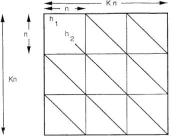
The matrix D is derived from the affine basis B. The vertices are stored in a dense array which is mapped onto a two-dimensional mesh of processors. Processing element (i, j) holds B,J, the ith component of the jth vertex. The Hessian is very sparse and has some special (K-diagonal) structure. Further-more, when the original problem [NLP] has a linear objective function, the nonzero diagonal vectors consist of identical subvectors (see Fig-are 1). Hence, only n out of the I-& x Kn entries of H need to be computed. This vector is stored in a one-dimensional array of processing elements. Operations on the Hessian, based on this one-dimensional mapping to the CM-2 processors, are explained below as we describe each computational module.

Computation of the Descent Direction. The most expensive computation of the master problem is the solution of the system

(DTHD)P =

–DTg.

(10)

The matrix DTHD could be computed in a straightforward manner by

computing first the product Y = HD and then the product D~ Y using the CMSSL matrix multiplication routine. However, this would require knowl-edge of the entire matrix H, whereas this is not necessary due to the special structure of H.

The computation of DT Y is straightforward to implement on the

Connec-tion Machine using the CMSSL routine GEN_MATRIX_MULT, which

oper-ates on the two dense matrices D and Y. However, we mention that the matrix D is not stored permanently on the CM-2. Instead it is computed as needed from the matrix of vertices B. In particular D ~ = B ~ – B , Vj =

1,....u – 1where B ~denotes the jth column of the matrix B. This operation is executed within microseconds by multiple processing elements,

We focus now on the product Y = HD that uses the sparse Hessian. We

visualize each matrix as a two-dimensional object with individual elements

t

n +

Only n entries of the HessIan matrix are stored

The remalnlng entries are Identical to the first n.

Fig. 1. The structure of the Hessian H.

laid out on a rectangular mesh of processors. The axis extents of the mesh are equal to the respective dimensions of the matrix. Two matrices having the

same shape (dimensions) are laid out so as to have their corresponding

entries on the same processor of the rectangular mesh. This scheme allows

the same computation involving all elements of the two matrices to be

performed concurrently in one step. The product Y = IUl is computed as

follows. Recall that D is a K-z X (u – 1) matrix.

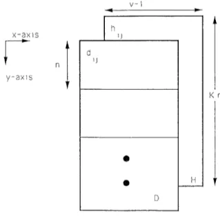
(1) Spread the vector of nonzero entries of H on the two-dimensional mesh that stores D. This vector is spread along the x-axis u – 1 times and along the y-axis K times. That is, H is translated into conformable dimensions (Krz x (v – 1)) as D.

(2) Perform elementwise multiplication, i.e., each processor (i, j) has access

(3)

(4)

to elements H,j an~ D,~ and performs the product H, JD,J and stores the result. The result YI is another Krz x (u – 1) matrix with K slices along the y-axis.

Accumulate a sum by superimposing each slice of the matrix YI to obtain a matrix Yz of dimension n x (v – 1).

Replicate the matrix ~z K times along the y-axis to get Y = IU1. We give a pictorial description in Figure 2. The corresponding CM Fortran code is given in the Appendix.

The Computation of the Gradient. The right-hand side of the linear

sys-tem (10) can be computed on the CM-2. The matrix D and the vector g are

542 . M. C. Pinar and S. A. Zenios \/-I 4 x-axis r _n y-axis

I

h )) H } n

Add all K sllces of the above elemeln:~~lse product to get {

cl=

Y n Y I HD e e 11 I 1

Fig. 2 Computing the product HD of the matrix DTHD on the CM-2.

stored on the CM, and the computation DTg is performed using the CMSSL

routine for matrix-vector multiplication.

Function and Gradient Evaluations. The function and gradient evalua-tions on the CM-2 are straightforward. First, we compute the linear objective function as an inner product of the cost vector and the current iterate. Next, we compute the function value contributed by the penalty function. In order ACM Transactionson MathematicalSoftware,Vol 20,No,4, December1994

to perform this computation the violation in the side constraint inequalities is

computed to determine whether the linear or the quadratic part of the

penalty function is appropriate for each GUB constraint. A parallel condi-tional construct then computes the quantity contributed to the objective

function by each GUB constraint. The corresponding CM Fortran code is

given in the Appendix.

The Computation of the New Iterate. We compute the new iterate x based on the simplicial weights w as

x =Bw. (11)

This is a dense matrix-vector product that is performed on the CM-2 using CMSSL routines.

4. NUMERICAL RESULTS AND DISCUSSION

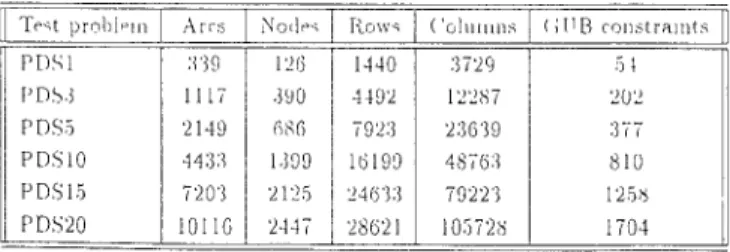
A set of numerical results using the Patient Distribution System (PDS)

problems are presented in this section. The PDS problems are linear

multi-commodity flow problems with 11 commodities [Carolan et al. 1990]. We

consider six problems. The characteristics of the test problems are given in Table I.

The purpose of this section is to illustrate the efficiency of the various algorithmic strategies we adopted and the effectiveness of the algorithm in solving large-scale problems. We also concentrate on issues that relate to the parallel implementation, like scalability and sustained FLOP rates.

4.1 Experiment 1: Efficiency of the Parallel Implementation

The dense linear algebra operations (Section 3.3) were expected to achieve high FLOPS rates on the CM-2. Unfortunately, the fact that the matrix D is “thin” (i.e., it has a large number of rows, but typically small number of columns that grows as vertices are added) degrades the performance of the

CMSSL routines. Table II illustrates the results. Using an alternative

matrix-multiplier routine by Johnsson and Ho [1987], streamlined for rectan-gular matrices, improves the performance of the master program routines by

a factor of 10. Even if the achieved FLOPS rate falls short of the peak

performance of the CM-2, it is still comparable to the performance achieved in the master program solver on the CR4Y Y-MP when the results are scaled to a 32K CM-2; see Pinar and Zenios [1992].

We report in Table III the solution statistics using the LQP algorithm on the CM-2. In the CM-2 experiments the rein-cost network flow subproblems

are solved on the front end Sun Workstation using the network simplex

algorithm. The CM Fortran code was compiled with –s 1i c ewis e option. The

computation was stopped when the absolute degree of infeasibility in the

joint capacity constraints was less than 10- 5. The objective function value reported on termination has four to five digits of accuracy compared to the

optimal values reported by the general-purpose linear programming code

MINOS for PDS1 and PDS3. This does not necessarily correspond to a similar agreement of the flow values reported by the respective codes. With PDS 1 for

544 . M. C, Plnar and S, A, Zenios

Table I. Test Problem Characterlstlcs Tmt prnl>l PIII P[)\l r’r)~ j F’D\j PD\lo PD5’15 Pr)\20 10I1G 2447 28621 lo572b I I 704

Table II. Sustained MFLOPS for the Master Program Routines Dnnension of D SK CM–2 MFLOP Rates

(<I1155L routines I Johnssou and Ho [1 I]

1 10’24 x 10’24 .126 162,

II,Ooox 1000 I 160

I

21:1

II

u

23639 X :]9 (P D5’5) 554 516

[111refers to Jolmsson and Ho [1987]

instance, although some flow values reported by MINOS and LQP fully agree, some differ significantly despite the five digits of accuracy in the objective function value.

We also solved the first four problems on a serial DEC Alpha 3000 AXP

Model 500 running OSF using a serial implementation of the linear-quadratic penalty algorithm; see Zenios et al. [1994]. The code was compiled using the

– o option of the f 77 compiler. Due to lack of memory, we were not able to solve PDS15 and PDS20. These results are also given in Table III. The times are given in hrs:mins:secs in all subsequent tables.

We notice that using the 32K CM-2 we are able to solve PDS 15 in the same time as we solve PDS1O on the DEC workstation. Furthermore, we are able to solve PDS20 in less than twice as much time on the CM-2, whereas a similar performance cannot be expected on the llEC workstation.

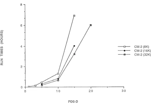
In Figure 3 we illustrate the scalability of the LQP algorithm on the data-level parallel architecture. In particular, it is encouraging to observe that PDS5 is solved on the 8K CM-2 in approximately the same time as the 32K CM-2 solves PDS1O. To understand why a fourfold increase in the number of processing elements is needed to achieve this result, whereas PDS 10 is only twice as large as PSD5, we make the following observation.

An important feature of the dense linear algebra computations in the master problem is the dynamic nature of the matrix ~. The column dimen-sion of the matrix D increases as the algorithm progresses and as more extreme points are used to represent the network feasible set X. Although

this feature enhances more effective processor usage, we cannot expect a

uniform scalability in this case. More precisely, at iteration k the algorithm processes a matrix of size, say q x k, instead of working on a matrix of ACM TransactIons on Mathematical Software, Vol 20, No 4, December 1994

Table III. Performance of the Data-Parallel Implementation of the Linear-Quadratic Penalty Algorithm on a 32K CM-2 System with Master Problem Computations on the CM-2 Compared to the

Performance of the Implementation of the Same Algorithm on the DEC Alpha 3000 AXP Model 500 (NA = Not Available)

Test Problem CM–2 (SK) CM–2 (16K) CM–2 (32K) DEC Alpha 3000

PDSI 0121 XA N A 010 PDS3 0?45 y~ N A 0848 PDS5 o ~T 27 01723 0100 05634 PDSIO 11s0 04842 0380 3120 PDS15 6540 414s 3120 NA PDS20 N/i VA 600 NA ————u——CM-2 (8K) — CM-2 (16K) ———u———CM-2 (32K) o 10 20 30 PDS-D

Fig. 3. Solution times for increasing problem sizes on the CM-2 as the number of processing elements M increased.

dimension q X q throughout the execution of the algorithm. If p processors are available to execute the LQP algorithm on a given multiprocessor system,

the execution time of two successive iterations of the LQP algorithm is

subject to variation as a result of the increasing size, whereas a more uniform execution time could be expected for the iterations in the latter case. We believe this feature of the LQP algorithm has a significant negative impact on the data-parallel performance as evidenced in Figure 3.

546 100 90 80 70 60 50 40 30 20 10

. M. C, Pinar and S A. Zenlos

The percentage distribution of the solution

time on the DEC Alpha 3000

PDS3 PDS5

❑

subproblem

3 D master

The percentage distribution of the solution time on the CM-2 32K 30 20 10 0 PDS3 PDS5

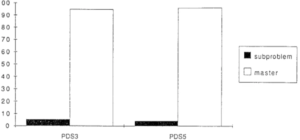
Fig, 4. The distribution of solution time between the subproblem and the master problem on the DEC Alpha 3000 and on the CM-2.

The distribution of the total solution time between the subproblem and the

master problem on the CM-2 and on the DEC workstation is illustrated in

Figure 4. We observe that the solution times on the CM-2 are balanced

between the subproblem and master program computations, whereas the

master program dominates on the DEC workstation by a large margin. ACM TransactIons on Mathematical Software, Vol 20, No 4, Dscember 1994

Table IV. Performance of the Linear-Quadratic Penalty Algorithm on a 16K CM-2 System with both Master Problem and Subproblem Computations on the CM-2

Test Problcrn Total time (QPPRA) Total time (Network Simplex) r

PDS1 080 0025

PDS3 0430 030

Unfeasibility Improvement vs. major iterations. 200 ~ 140 100 80

T

=

60 -40 1 0 1 ~2-—--z~2. 1 2 3 4 5 6 7 8

Number of major iterations

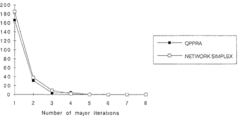
Fig. 5. Progress of the LQP algorithm with (1) QPPRA and (2) Network Simplex illustrated using PDS1.

4.2 Experiment 2: The Effect of Subproblem Solver

The quadratic proximal point/row-action (QPPRA) algorithm of Nielsen and

Zenios [1993] is used to solve the linear network subproblems on the CM-2.

To solve the linear network problems, the QPPRA code is called as a

subroutine. Since QPPRA was written in C/PARIS (Parallel Instruction Set),

a CM Fortran C/PARIS interface was built to link the LQP code with the

QPPRA solver. To solve the independent rein-cost network flow problem for each commodity simultaneously, the problem data is rearranged as a single rein-cost network problem consisting of independent rein-cost networks. The computational results are summarized in Table IV. We report the total time to solve each test problem to an absolute degree of infeasibility of 10-3. On the new Connection Machine CM-5 it is possible to solve the subproblems on multiple processors, using the network simplex solver. This would require use

of the CM-5 as an SIMD system for the master program and as an MIMD

system for the subproblems. One encouraging point is that using the QPPRA solver does not impair the progress of the LQP algorithm in terms of reducing the degree of infeasibility in the GUB constraints and the number of itera-tions to termination. In Figure 5, we plot the infeasibility error versus the

548 . M. C. Pinar and S. A. Zenios

number of major iterations (i.e., the number of executions of Step 1 of the LQP algorithm) when (1) the network simplex was used on the front end and (2) the QPPRA replaces the network simplex solver.

4.3 Experiment 3: Benchmarks on the CM-5

Thinking Machines Corporation has recently introduced the Connection

Ma-chine CM-5. This system integrates features of both SIMD and MIMD

architectures. It is based on a network of RISC workstations, each enhanced with vector functional units. (The architecture is presumably scalable up to

16,000 workstations, each delivering 128 MFLOPS peak performance.) The

CM-5 can be programmed in SIMD mode, whereby problem data are

dis-tributed among multiple workstations, and they all execute identical instruc-tions on their data set. In this mode of computing the CM-5 is compatible

with the CM-2. Hence, we could use the LQP implementation to benchmark

the performance of this new architecture.

We ran the LQP algorithm, with the network simplex solvers, on the CM-5.

Results are summarized in Table V for a 256- and 512-processor CM-5. We

expect that substantial improvements will be realized when the CM-5 is fully operational with vector functional units.

Additional improvements in the performance of the algorithm are possible with the parallel solution of the rein-cost network subproblems on multiple nodes of the CM-5. The LQP algorithm matches nicely to this new architec-ture. In particular, it can exploit the SIMD capabilities in solving the dense master problem. Subproblems can be solved using the MIMD capabilities and the more efficient simplex solver.

4.4 Comparisons

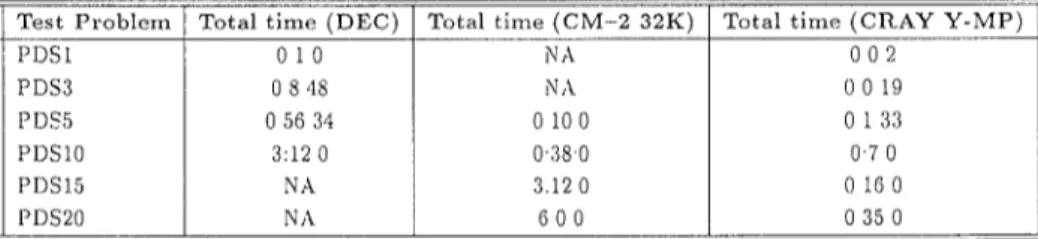
We summarize in Table VI the performance of the data-level parallel LQP

algorithm, against its implementation on a serial computer, the DEC Alpha

3000 AXP, and against the performance of the vectorized algorithm on the

CRAY Y-MP as implemented by Pinar and Zenios [ 1992].

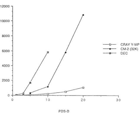
A comparison of solution times is plotted in Figure 6 where the solution

time of PDS1 on the CRAY Y-MP was taken to be unity, and the runtimes of

all problems on various architectures were normalized accordingly. We ob-serve that with respect to solution time the CM-2 results do not compare

favorably with the computational results obtained on the CRAY Y-MP. The

main reasons for this are the following,

(1) The “thin” shape of the matrix D affects the performance of

matrix-matrix and matrix-vector operations on both CM systems. Best

perfor-mance results are achieved when matrices satisfy certain shape require-ments.

(2) Communication costs are incurred during the SPREAD and

REPLI-CATE operations. The SPREAD operation takes as argument an array

and creates another array with an extra dimension. The REPLICATE

operation takes an array and replicates the entries along a given dimen-ACM TransactIons on Mathematical Software, Vol 20, No 4, December 1994

Table V. Performance of the Linear-Quadratic Penalty Algorithm on the CM-5 System with the Master Problem Executed on the CM-5 and Subproblem Computations Executed on the FE

(NA = Not Available)

~

Total time (256 proc. ) Total time (512 proc. )

Table VI. Performance of the Linear-Quadratic Penalty Algorithm on Various Architectures (NA = Not Available)

r

Test Problem PDS1 PDS3 pDS~ PDS1O PDS15 PDS20

Total time (DEC) 010 0848 05634 3120 XA N A Total time (CM-2 32K) N A !\l,i 0100 0380 3120 600

T

Total time (CRAY Y-MP) 002 0019 0133 070 0160 0350

sion. Both operations are used extensively in the computation of the

descent direction and result in interprocessor communication.

(3) Moving data among CM-2 arrays of different sizes also results in inter-processor communication.

(4) The dynamic structure of D affects the scalability negatively.

Nevertheless, as a first attempt to build a solver for multicommodity flows on a data-level parallel computer system, the results are still encouraging. In

particular, we see substantial improvements in performance over the DEC

workstation. Another advantage of the algorithm is its scalability, when

implemented on the MP architecture. We also remark that Zenios [1991]

developed a specialization of the row-action algorithms of Censor and Lent

[1981] to solve quadratic multicommodity transportation problems on the

Connection Machines CM-2 and CM-5. Although our algorithm is not a

“truly” MP algorithm like the row-action-type algorithms, it is one of the first

general-purpose decomposition methodologies implemented on the

Connec-tion Machines and, as such, removes the strict convexity requirements stated in Zenios [1991] by enabling the solution of linear programs.

5. SUMMARY AND CONCLUSIONS

We have reported on the data-level parallel implementation of the LQP

algorithm for multicommodity network flow problems. This is the most

550 . M, C. Pinar and S, A, Zenlos

ACOMPARISON OFRUN TIMES ON DIFFERENT PLATFORMS 12000

1

———Q———GRAY ‘i-MP e CM-2 (32K) ~ DEC J 10000- 8000- 6000-4000 2000 0 I i o 10 20 30 PDS-D

Fig. 6. A comparmon of normalized solution times for LQP on different architectures (the runtlme of PDS 1 on the CRAY Y-MP is taken as the unit of time),

general-purpose optimization algorithm that has been developed on an MP

architecture. Most earlier works have concentrated on either nonlinear, strictly convex programs, or emphasized more specialized structures, like assignment, transportation, rein-cost network flows, etc.

The data-level parallel implementation is substantially faster than a serial implementation of the algorithm. However, the data-parallel implementation does not compete favorably with the implementation of the algorithm on the CRAY Y-MP vector supercomputer. A very attractive feature of the data-level implementation, nevertheless, is its scalability. We expect that the algorithm could be substantially improved by exploiting some of the architectural features of the CM-5, like the vector units and the MIMD capabilities. It is quite interesting that the LQP algorithm combines features of both fine-grain (master program) and coarse-grain (subprogram) decomposition algorithms.

Another aspect of the algorithm that deserves further investigation is the

question of accuracy. The algorithm is an exterior-point algorithm that

attains feasibility on termination. The progress toward the feasible boundary is fast in the beginning, but slows down gradually. Furthermore, the quality of the solution on termination cannot be assessed unless a comparison with a ACM TransactIonson MathematicalSoftware,Vol 20,NO 4, December1994

more accurate algorithm is made. More research is needed to overcome these difficulties. Nevertheless, the algorithm was able to solve all test problems to

obtain an absolute feasibility error of 10-5, and produce objective function values that agree within five decimal points with an exact solution.

APPENDIX

The computation of the product Y = HD in CM Fortran is given below.

c–– ncom = number of commodities c–– nvml = number of vertices – 1

c–– spread H along D and perform multiplication

d = d * spread(replicate(h_cm, dim = 1,ncopies = ncom), $ dim = 2,ncopies = nvml) c–- perform summation dh2 = 0.0 do 100 i = 1,ncom dh2 = dh2+d((i -l)*na+l:i*na,:) 100 continue c–– replicate to get Y d = 0.0

d = replicate(dh2, dim = 1, ncopies = ncom) c–– compute C

call gen_matrix_mult(c, dt,d,l ,2,ier)

The function and gradient evaluation code segment is given below.

c–– above.. array where side constraint values are stored c Its value is O if constraint is satisfied.

c–– linear objective function computed as a dot product obj_cm = dotproduct(xl _cm,cost_cm)

c–– the nonseparable penalty function terms gradient = 0.0

where (above .gt. epsi) c–– constraint in the linear region

above = mu* (above - epsi / 2) gradient = mu

elsewhere

c–– _{constraint in the quadratic region} gradient = mu* (above/ epsi) above = mu* (above* *2)/(2* epsi) end where

c–– the value of the objective function = linear part + penalty terms obj-cm = obj_cm + sum(above)

g-cm = cost_cm + replicate(gradlent, dim = 1,ncopies = ncom)

ACKNOWLEDGMENTS

The assistance of J. Eckstein with the CM-2 experiments is gratefully

ac-knowledged. S. Nielsen kindly made available his programming skills during the development of the C/Paris-CM Fortran interface. The CM-2 computing

resources were provided through the support of AHPCRC, University of

Minnesota. The manuscript benefited from the comments of M. Saunders and

an anonymous referee.

552 . M, C. Plnar and S. A. Zenlos REFERENCES

ASSAD, A. A. 1978. Multlcommodlty network flows-a survey. Networks 8, 37-91.

BERTS~KAS, D. P. AND TSITSIKLIS, J. N. 1990. Parallel and Distributed Computation: Numerical Methods Prentice-Hall, Englewood Cliffs, N.J

BERTSEKAS, D, P., CAST.MiON, D., ECKSTEIN, J,, AND ZENIOS, S. A. 1994. Parallel computing in network optimization. In Handbooks m Operations Research, North-Holland, Amsterdam. To be published.

BLELLOCH, G. E. 1990. Vector Models for Data-parallel Computing. The MIT Press, Cambridge, Mass

CAROLAN, W. J., HILL, J. E., KENNINGTON, J. L., NIEMI, S., AND WICHMANN, S. J. 1990. An empirical evaluation of the KORBX algorithms for military airlift applications. Oper Res. 38, 240-248.

CENSOR, Y. AND LENT, A. 1981. An lteratlve row-action method for interval convex program-ming, J. Optlm. Theory Appl. 34, 321–353.

CENSOR, Y. AND ZENIOS, S.A. 1993. Theproximal minimization algorithm with D-functions. J. Optlm. Theory Appl. 73,455-468.

HEARN, D, W., LAWPHONGPANICH, S., AND VENTURA, J. A. 1987. Restricted slmplicial decomposi-tion. Computation and extensions Math Program Study 31, 99–1 18

HILLIS) W. D, 1985. The Connection Machine. The MIT Pressj Cambridge, Mass.

JOHNSSON, S. L. AND Ho, C. T. 1987. Algorithms for multiplying matrices of arbitrary shapes using shared memory primitwes on boolean cubes, YALEU/DCS /TR-569, Dept. of Computer Science, Yale Univ., New Haven, Corm.

KENNINGTON, J L. 1978. A survey of hnear multlcommodlty network flows, Oper. Res, 26, 209-236.

KENNINGTON, J. L, AND HELGASON, R. V, 1980. Algorithms for Network Programming. Wiley-Interscience, New York

MULVEY, J. M., ZENIOS, S. A,, AND AHLFELD, D. P, 1990. Slmpliclal decomposition for convex generalized networks. J In~ OptLm Set. 11, 359-387,

NIELSEN, S. N. AND ZENIOS, S. A 1993 Proximal minimizations with D-Functions and the massively parallel solutlon of hnear network programs. Comput, OptLm. Appl. 1, 375–398. NIELSEN, S. N, AND ZENIOS, S. A. 1992, Massively parallel algorithms for singly constrained

nonlinear programs ORSA J. Comput. 4, 166– 181.

PINAR, M ~. AND ZENIOS, S. A. 1994. On smoothing exact penalty functions for convex constrained optimization. SIAM J, Optlm. 4, 3, 486–5 11,

PINAR, M, ~. AND ZENIOS, S. A. 1992. Parallel decomposition of multlcommodity network flows using linear-quadratic penalty functions. ORSA J, Comput. 4, 235–249.

ROCRAFELLAR, T. R. 1976a. Augmented Lagrangians and apphcatlons to proximal point algo-rithms m convex programmmg. Math. Oper, Res. 1, 97– 116,

ROCKAFELLAR, T. R 1976b Monotone operators and the proximal point algorithm SIAM J, Control Optlm. 14, 877-898

SCHULTZ, G. L, AND MEYER, R, R. 1991. An mterlor point method for block angular optlmlzatlon. SIAM J. Opttm. 1.583-602.

VON HOHENBALKEN, B. 1977 Ehmplicial decomposition in nonlinear programming algorithms. Math Program. 13, 49-68.

ZENIOS, A. S. 1991. On the fine-gram decomposition of multlcommodlty transportation prob-lems SIAM J Optlm. 1, 643-669

ZENIOS, S. A. AND LASKEN, R. A. 1988. Nonlinear network optimization on a massively parallel Connection Machine. Ann Oper. Res, 14, 147-165

ZENIOS, S. A., PINAR, M. ~., AND DEMBO, R. S. 1994, A smooth penalty function algorithm for network structured problems. Eur. J. Oper Res To be published.

Recewed December 1993; revised August and October 1993; accepted December 1993