D O I: 1 0 .1 5 0 1 / C o m m u a 1 _ 0 0 0 0 0 0 0 7 3 4 IS S N 1 3 0 3 –5 9 9 1
MODELING OF CAPACITY UTILIZATION RATIO WITH FUZZY TIME SERIES BASED ON MARKOV TRANSITION MATRIX
H·ILAL GÜNEY AND M.AK·IF BAKIR
Abstract. Modeling of time series with fuzzy logic has found an increasingly expanding usage in recent years. One of the most important reasons for this is that fuzzy logic approach doesn’t require assumptions needed by the typical time series. Inclusion of the some weightings and probability calculations at the forecast stage into the …rst studies starting through the modeling of time series with fuzzy logic resulted in further improvement of the forecast quality. Tsaur (2011) achieved better forecasted results by including the Markov transition probabilities matrix. Fuzzy time series is also an approach which can be ‡exibly used in various model structures as it easily overcomes the di¢ culties caused by the model structure - linear or non-linear form. In this study, Markov method of Tsaur is applied on the monthly capacity utilization ratio (CUR) of Turkey which has a non-linear structure and free of seasonality belonging to the period between 2007-2015. In this sense, the results are compared to the results of SETAR model and it’s seen that Tsaur’s approach has provided better results compared to the forecasts of typical time series.
1. Introduction
Particularly, in cases of time series not showing a regular pattern, it’s quite dif-…cult to create an adequate time series model. In such a case, more prior studies should be conducted: to search for the presence of unit root in the series, to look whether there is structural break, examine stationarity of the series, and to deter-mine the approximate behavior of data etc. This kind of prior studies increases the work load in modeling of time series. While all initial studies increase the work load, it makes the modeling di¢ cult that particularly in cases of data not show-ing regular behavior pattern, forecastshow-ing with typical time series approach require satisfying the assumptions. When time series analysis is performed by using fuzzy logic, the series is analyzed based on the information obtained from the behavior of the relevant data in time. Not requiring assumptions regarding the series and its applicability, in particular, small sample size satisfactorily are the most important advantage provided by the fuzzy time series approach.
Received by the editors: June 26, 2015, Accepted: October 15, 2015.
Key words and phrases. Markov, Fuzzy Time Series, Forecast, Non-Linear Time Series.
c 2 0 1 5 A n ka ra U n ive rsity
De…ned by Zadeh for the …rst time in 1965, the fuzzy set is the set of elements with continuous membership degrees. Fuzzy set is characterized with the member-ship function that assigns membermember-ship degree to each element between 0-1. It’s developed against the binary logic system as ”An object is whether the element of the set or not” based on the Aristotle’s logic. Fuzzy logic is a logic system that determines at which degree the object is an element of the set by assigning mem-bership degrees to the event of object being an element of a set (Zadeh, 1965). Fuzzy systems generally consist of three basic phases as fuzzylising, fuzzy inference and defuzzifying (Aladag and Turksen, 2015). Fuzzy time series analysis is sort of fuzzy system. Fuzzylising means the assignment of time series observations to the fuzzy sets with certain membership degrees. In other words, it corresponds to the determination of lengths of interval. The phase of fuzzy inference is the determi-nation of fuzzy relationships. Defuzzifying is, on the other hand, a process which converts the fuzzy set or fuzzy number into a crisp number.
Song and Chissom (1991) used a …xed length of interval and fuzzy relationship matrix in their …rst study in which they proposed the …rst degree fuzzy time series model. Chen (1996) proposed a simpler fuzzy time series approach for the com-plicated matrix manipulation of Song and Chissom (1991). The biggest di¤erence between these two studies is that Chen does not use membership degree, and makes forecast by classifying the fuzzy relationships. As this method proposed by Chen has ease of application, it has become one of the most preferred methods in the literature. Although Hwang et al. (1998) divided universe of discourse with a …xed length of interval, he fuzzy…ed the …rst degree di¤erence of the data instead of fuzzifying the data. Huarng (2001) discussed that the …rst degree di¤erence of the series method gives better forecasts comparing with randomly choosing the length of interval. Tsaur et al. (2005) considered the entropy as fuzziness measure, and achieved fuzzy relationship matrix with the help of entropy. Yu (2005-a) claimed that it will provide better forecasted results to give di¤erent weights according to the importance levels instead of taking repeated relationships only once. Yu (2005-b) apply fuzzy correction on Chen’s model for adjusting fuzzy relationships to propose a new fuzzy time series model. Thus, he achived better forecasted re-sults than Chen’s forecasts by additionally taking into account this fuzzy correction instead of centroid method in defuzzify process. Huarng and Yu (2006) de…ned the length of interval with percentile values by taking relative di¤erences of observation values. They showed that length of interval based on ratio gives better forecasted results than distribution and average based length of interval. In the study in which Cheng et al. (2008) used adaptive expectation model, after making fuzzy time se-ries forecast with weighted model in Yu (2005), they adjusted the forecasted results with adaptive expectation. Yolcu et al. (2009) used single variable constrained optimization to determine the length of interval, and thus, improved the ratio and average based method of Huarng. The proposed method needs less procedures as it does not require relative di¤erence. E¼grio¼glu et al. (2009) o¤ered an approach
with higher performance by combining SARIMA models with seasonal fuzzy time series models for the analysis of seasonal fuzzy time series. In this method, they used feed-forward arti…cial neural network to determine the fuzzy relationships. Al-ada¼g et al. (2009) established fuzzy relationships for higher-degree AR models with feed-forward arti…cial neural network. Aladag et al. (2010), in another study, tried adaptive expectation in higher-degree fuzzy time series models. Tsaur (2011) used Markov chain transition matrix to achieve fuzzy relationship groups. This method that is applied for …rst degree fuzzy time series calculated observation frequencies of repeated relationships, and subsequently considered these frequencies as repeti-tion probabilities of the relarepeti-tionships, and created transirepeti-tion matrix from state i to state j. at the …nal stage he corrects the forecasts through this transition matrix according to the Markov transition process. Thus, he showed superiority to many methods available in the literature in terms of forecasting performance.
This study is interested in modeling of capacity utilization ratio (CUR) data with a length of n=97 for Turkey and between years 2007-2015. The data is seasonally adjusted and has a non-linear behavior. The examination of data shows that while there is a decreasing trend from 1st month of 2007 until 7th month of 2008 with a rapid decrease from 8th month of 2008, the series started to increase after the 4th month of 2009, and stabilize following 10th month of 2010. As the data does not behave in a linear form, it will not be adequate to approach by linear time series models. Self-existing threshold autoregressive (SETAR) would be an appropriate modeling approach for the data with this pattern. Although, a non-linearity is apparently seen in this data, only reviewing the diagram may sometimes cause misinterpretation. Thus, a preliminary study for more accurate decision about non-linearity through a statistical tests would be well. In this study, Tsaur‘s …rst degree fuzzy time series approach with Markov transition matrix is applied on our data. To evaluate the performance of this approach in modeling the considered data, it also has been analyzed with SETAR model complying with the form of data. As a result of the comparison made, it’s seen that …rst degree fuzzy time series approach of Tsaur (2011) based on Markov transition matrix gives better forecast performance. It stands out as an important …nding that fuzzy time series approach based on Markov transition matrix that does not require many prior process and statistical tests as typical approaches produces quite good forecasts also for a real life data.
The following part of the study includes basic de…nitions and refers to essential characteristics of Tsaur’s method. In the 3rd part, analysis of the studied data with Tsaur’s method is explained in detail. In the traditional time series analysis of data, …rstly, some statistical tests are conducted to see that a SETAR model approach is appropriate. Performance comparison of these two methods is made by calculating MAPE (mean absolute percentage error) values of the forecasts.
2. Tsaur’s Markov Model
Before mentioning about Tsaur’s model, it will be useful to provide basic de…n-itions regarding …rst-degree fuzzy time series.
Let U be the universe of discourse, U = fu1; u2; :::; ung. A fuzzy set A of Uis
de…ned by A = fA(u1)/u 1+ fA (u2)/u 2+ ::: + fA (un)/u n (1)
where fAis the membership function of A, fAi : U ! [0; 1], and fA(ui) indicates the grade of membership of uiin A, where fA(ui) 2 [0; 1] and 1 i n. The basic
de…nitions of fuzzy time series can be summarized as follows (Song and Chissom 1991; Song and Chissom 1993).
De…nition 1. Let Yt 2 R1 (t = 0; 1; 2; :::) be a time series. If fi(t) a fuzzy set
in Yt and F (t) = ff1(t); f2(t); :::g, then F (t) is called a fuzzy time series in Yt.
De…nition 2. Suppose F (t) is caused by F (t 1) only, i.e., F (t 1) ! F (t). Then this relation can be expressed as F (t) = F (t 1) R(t; t 1) where R(t; t 1) is a fuzzy relationship, and is called the …rst-order model of F (t).
Chen (1996) emphasized the complexity of fuzzy matrix processes in his study and proposed a simple algorithm. In the method, …rst universe of discourse is de…ned as to cover all data, and, universe of discourse is divided into equal intervals according to the number of linguistic variables. After the data fuzzy…ed with the help of fuzzy sets de…ned on the universe of discourse, fuzzy logical relationships are created and classi…cation is made according to the left sides of these relationships. Then, the fuzzy forecasts are defuzzy…ed with average method.
In Tsaur’s (2011) method, in addition to Chen’s algorithm, Markov chain tran-sition matrix is used when relationship groups are obtained. This method applied for …rst degree fuzzy time series considers repeated relationships depending on a probability, and has the superiority in forecasted values over the many methods in the literature by making corrections in the forecasts through the transition matrix. In the study, the well-known data of student enrollment in Alabama University is used. In his method, universe of discourse is de…ned as to cover all data, and then universe of discourse is divided into equal intervals to create fuzzy sets. Following the fuzzi…cation, the process follows two steps of operations: fuzzy logical rela-tionships are de…ned, and then Markov transition probabilities matrix is created according these relationships. The forecasts obtained by using Markov transition probabilities matrix are corrected with Markov transition process diagram. This calculation process can be summarized algorithmically as follows:
(1) De…ne the universe of discourse.
(2) Divide universe of discourse into equal intervals, and de…ne fuzzy sets. (3) Fuzzify the historical data.
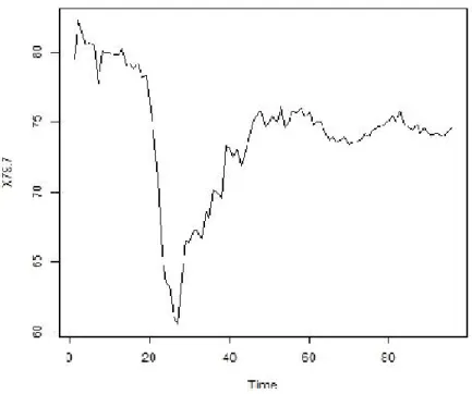
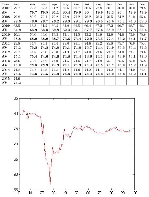
Figure 1. Industry (CUR) and Seasonally Adjusted CUR* (Weighted Average - %.
(5) Establish Markov state transition matrix, and then, draw transition process diagram from fuzzy logical relationships.
(6) Calculate the forecasted output by using Markov state transition matrix. (7) Adjust the tendency of the forecasted values.
3. Fuzzy Time Series Forecasting of Capacity Utilization Ratio Data Capacity utilization ratio (CUR) data including 97 observations considered here is published on the website of Central Bank of Republic of Turkey. Non-linear, and interesting structure of the data can be seen in the plot in Figure 1. CUR data shows di¤erent behaviors in di¤erent period intervals. The estimation process will be conducted at two subsequent stages: forecasting with fuzzy time series method of Tsaur based on Markov matrix, and then SETAR model. Finally, we will evaluate the performances of these two methods are compared via their MAPE’s. All calculations are performed in R package program.
For CUR data in Table 1, to calculate …rst degree fuzzy time series, …rst frequency of repeated relationships is calculated, and then, these frequencies are employed as repetition probabilities of the relationships. Transition matrix from state i to statej is created by replacing the calculated probabilities. Finally, forecasts made with this matrix are corrected, and, thus, improved by considering the Markov transition process diagram. The required calculations are given through the following steps.
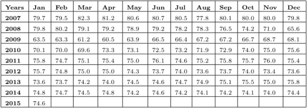
Table 1. Utilization Rate of Manufacturing Industry (CUR) and Seasonally Adjusted CUR* (Weighted Average - %)
Years Jan Feb Mar Apr May Jun Jul Aug Sep Oct Nov Dec
2007 79:7 79:5 82:3 81:2 80:6 80:7 80:5 77:8 80:1 80:0 80:0 79:8 2008 79:8 80:2 79:1 79:2 78:9 79:2 78:2 78:3 76:5 74:2 71:0 65:6 2009 63:5 63:3 61:2 60:5 63:9 66:5 66:4 67:2 67:2 66:7 68:7 68:1 2010 70:1 70:0 69:6 73:3 73:1 72:5 73:2 71:9 72:9 74:0 75:0 75:6 2011 75:8 74:7 75:1 75:4 75:0 76:1 74:6 75:2 75:8 75:7 76:0 75:4 2012 75:7 74:8 75:0 75:0 74:3 73:7 74:0 73:6 73:7 74:0 73:4 73:6 2013 73:6 73:7 74:2 74:0 74:5 74:6 74:7 74:9 75:1 75:5 75:0 75:8 2014 74:8 74:7 74:5 74:8 74:2 74:6 74:2 74:1 74:2 74:1 74:0 74:4 2015 74:6
Step 1. De…nition of universe of discourse: The universe of discourse is U = [Dmin D1; Dmax+ D2], where Dmin= 60:5 and Dmax= 82:3 denote the minimum
and maximum values of data set respectively. D1and D2are selected as to cover
all data of universe of discourse of CUR data. Thus, D1 = 0:5 and D2 = 0:7
are arbitrarily selected, and now the universe of discourse can be written as U = [60; 83].
Step 2. De…nition of fuzzy sets: Universe of discourse U = [60; 83] is divided into intervals according to the personal experience. Here, class number is supposed 8, and therefore, dividing the universe of discourse into 8 equal intervals. This results in the following sub-intervals:
u1= [60 ; 62:875] u2= [62:875 ; 65:75] u3= [65:75 ; 68:625] u4= [68:625 ; 71:5] u5= [71:5 ; 74:375] u6= [74:375 ; 77:25] u7= [77:25 ; 80:125] u8= [80:125 ; 83]
Depending on sub-intervals of universe of discourse U , A1; A2; A3; :::; A8 fuzzy
A1= 1/u1+ 0:5/u2+ 0/u3+ 0/u4+ 0/u5+ 0/u6+ 0/u7+ 0/u8
A2= 0:5/u1+ 1/u2+ 0:5/u3+ 0/u4+ 0/u5+ 0/u6+ 0/u7+ 0/u8
A3= 0/u1+ 0:5/u2+ 1/u3+ 0:5/u4+ 0/u5+ 0/u6+ 0/u7+ 0/u8
A4= 0/u1+ 0/u2+ 0:5/u3+ 1/u4+ 0:5/u5+ 0/u6+ 0/u7+ 0/u8
A5= 0/u1+ 0/u2+ 0/u3+ 0:5/u4+ 1/u5+ 0:5/u6+ 0/u7+ 0/u8
A6= 0/u1+ 0/u2+ 0/u3+ 0/u4+ 0:5/u5+ 1/u6+ 0:5/u7+ 0/u8
A7= 0/u1+ 0/u2+ 0/u3+ 0/u4+ 0/u5+ 0:5/u6+ 1/u7+ 0:5/u8
A8= 0/u1+ 0/u2+ 0/u3+ 0/u4+ 0/u5+ 0/u6+ 0:5/u7+ 1/u8
Here, ui in the denominator of fuzzy sets Ai are sub-intervals, while numbers in
nominator denote membership degrees of ui to Ai, subject to 0 ui 1.
Step 3. Fuzzi…cation of data: CUR data should be fuzzy…ed according to the biggest membership degree. If the highest membership degree of data appears in fuzzy setAk, the corresponding data is fuzzy…ed asAk. For example, the data
of January 2007, (79.7) is a value falling into sub-interval u7. As the highest
membership degree of the sub-interval u7is in A7, this value is fuzzy…ed as A7. Set
of values that are fuzzy…ed in similar manner are given in Table 2. Table 2. Fuzzy…ed Utilization Rate of Manufacturing Industry (CUR) data
Years Jan Feb Mar Apr May Jun Jul Aug Sep Oct Nov Dec
2007 79.7 79.5 82.3 81.2 80.6 80.7 80.5 77.8 80.1 80.0 80.0 79.8 Fuzzy…ed A7 A7 A8 A8 A8 A8 A8 A7 A7 A7 A7 A7 2008 79.8 80.2 79.1 79.2 78.9 79.2 78.2 78.3 76.5 74.2 71.0 65.6 Fuzzy…ed A7 A8 A7 A7 A7 A7 A7 A7 A6 A5 A4 A2 2009 63.5 63.3 61.2 60.5 63.9 66.5 66.4 67.2 67.2 66.7 68.7 68.1 Fuzzy…ed A2 A2 A1 A1 A2 A3 A3 A3 A3 A3 A4 A3 2010 70.1 70.0 69.6 73.3 73.1 72.5 73.2 71.9 72.9 74.0 75.0 75.6 Fuzzy…ed A4 A4 A4 A5 A5 A5 A5 A5 A5 A5 A6 A6 2011 75.8 74.7 75.1 75.4 75.0 76.1 74.6 75.2 75.8 75.7 76.0 75.4 Fuzzy…ed A6 A6 A6 A6 A6 A6 A6 A6 A6 A6 A6 A6 2012 75.7 74.8 75.0 75.0 74.3 73.7 74.0 73.6 73.7 74.0 73.4 73.6 Fuzzy…ed A6 A6 A6 A6 A5 A5 A5 A5 A5 A5 A5 A5 2013 73.6 73.7 74.2 74.0 74.5 74.6 74.7 74.9 75.1 75.5 75.0 75.8 Fuzzy…ed A5 A5 A6 A5 A6 A6 A6 A6 A6 A6 A5 A6 2014 74.8 74.7 74.5 74.8 74.2 74.6 74.2 74.1 74.2 74.1 74.0 74.4 Fuzzy…ed A6 A6 A6 A6 A5 A6 A5 A5 A5 A5 A5 A6 2015 74.6 Fuzzy…ed A6
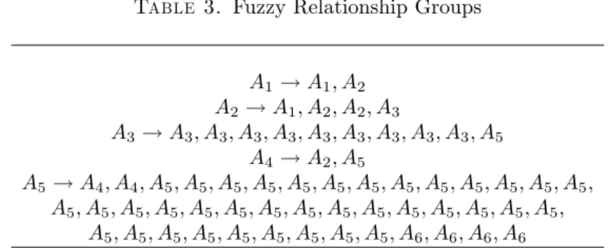
Step 4. De…nition of fuzzy logic relationships: In this step, fuzzy logical re-lationships are de…ned between the fuzzy…ed data, and then, fuzzy relationship groups are formed. Classi…cation process is performed based on the current status of the fuzzy logical relationships. All de…ned fuzzy relationship groups are listed in Table 3.
Step 5. Establish Markov state transition matrix and transition process: Tran-sition probabilities matrix P is obtained by using from the fuzzy relationships in
Table 3. Fuzzy Relationship Groups A1! A1; A2 A2! A1; A2; A2; A3 A3! A3; A3; A3; A3; A3; A3; A3; A3; A3; A5 A4! A2; A5 A5! A4; A4; A5; A5; A5; A5; A5; A5; A5; A5; A5; A5; A5; A5; A5; A5; A5; A5; A5; A5; A5; A5; A5; A5; A5; A5; A5; A5; A5; A5; A5; A5; A5; A5; A5; A5; A5; A5; A5; A6; A6; A6; A6
Step 4. De…ning n states (8 states) for each one of the fuzzy sets, nxn (8x8) di-mensional matrix is produced. State transition probabilities Pij, from state Ai to
state Aj in one step, are calculated with equality
Pij =
Mij
Mi
i; j = 1; 2; :::; n
Here, Mij and Mi denote transition time in one step from state Ai to stateAj, and
data amount in state Ai respectively. Thus, Markov transition probabilities matrix
Pij becomes Pij= 2 6 6 6 6 4 P11 P12 ::: ::: P1n P21 P22 ::: ::: P2n ::: ::: ::: ::: ::: ::: ::: ::: ::: ::: Pn1 Pn2 ::: ::: Pnn 3 7 7 7 7 5 For CUR data, transition probabilities are given below.
P = 2 6 6 6 6 6 6 6 6 6 6 6 4 1/2 1/2 0 0 0 0 0 0 1/4 2/4 1/4 0 0 0 0 0 0 0 2/3 1/3 0 0 0 0 0 1/5 1/5 2/5 1/5 0 0 0 0 0 0 1/26 21/26 0 0 0 0 0 0 0 4/33 29/33 0 0 0 0 0 0 0 1/14 11/14 2/14 0 0 0 0 0 0 1/3 2/3 3 7 7 7 7 7 7 7 7 7 7 7 5
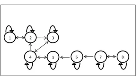
Markov matrix given above will be used to create Markov transition probabilities diagram in Figure 3.
Step 6. Calculation of forecasted values: Fuzzy forecasting is conducted regard-ing two cases: one-to-one and one-to-many. Followregard-ing rules given by Tsaur (2011) are taken into account in these calculations.
Figure 2. Transition process
One-to-one: If the fuzzy logical relationship group of Aiis one-to-one (i.e.,
Ai! Ak, with Pik= 1 and Pij = 0, j 6= k), then the forecasting of F (t) is
mk, the midpoint of uk, according to the equation F (t) = mkPik= mk.
One-to-many: If the fuzzy logical relationship group of Aj is one-to-many
(i.e., Ai ! A1; A2; :::An; j = 1; 2; :::; n), when collected data Y (t 1) at
time (t 1) is in the state Aj, then the forecasting of F (t) is equal to F (t) =
m1Pj1+m2Pj2+:::+mj 1Pj(j 1)+Y (t 1) Pjj+mj+1Pj(j+1)+:::+mnPjn
, where m1; m2; :::; mj 1; mj; :::; mn are the midpoint of u1; u2; :::; uj 1;
uj; :::; un, and mj is substituted for Y (t 1) in order to have more
infor-mation from the state Aj at time (t 1).
For example, the forecasted value for 2nd month in 2007 is calculated as follows: F (2007 : 2) = 1 14m6+ 11 14Y (2007 : 1) + 2 14m8 F (2007 : 2) = 1 1475:8125 + 11 1479:7 + 2 1481:5625 = 79:68839 79:7
Step 7. Adjusting forecasted values: For series with small sample size estimated Markov chain matrix is usually biased, and some adjustments for the forecasts are suggested to revise the forecasting errors for one-to-many cases. First, in a fuzzy logical group where Ai communicates with Ai and Aj for i 6= j,j = 1; 2; :::; n. If
a larger state Aj is accessible from state Ai, then the forecasting value for Aj is
usually underestimated because the lower state values are used for forecasting the value of Aj. On the other hand, an overestimated value should be adjusted for the
forecasting value Ajbecause a smaller state Ajis accessible from Ai, i; j = 1; 2; :::; n.
jumps backward to state Ai k(k 2), then it is necessary to adjust the trend of
the pre-obtained forecasting value. Thus, we have smoother values of forecasting. Corrections are made by taking into account some of the following rules. To understand the rules better, …rst of all necessary de…nitions are given.
Before giving the correction rules suggested by Tsaur (2011), let us give to nec-essary de…nitions.
De…nition 3. If Pij > 0, then state Aj is accessible fromAi, Ai! Aj.
De…nition 4. If states Ai and Aj are accessible to each other, then Ai
communi-cates withAj, Ai$ Aj.
Now, the corrections are made by taking into account the following rules. If Ai$ Aj, starting in state Aiat time (t 1) as F (t 1) = Ai, and makes
an increasing transition into state Aj at time t, (i < j), then the adjusted
trend value Dtis de…ned as Dt1 = l/2 .
If Ai$ Aj, starting in state Aiat time (t 1) as F (t 1) = Ai, and makes
an decreasing transition into state Aj at time t, (i > j), then the adjusted
Dt is de…ned as Dt1= l/2 .
If the current state is in the state Ai at time (t 1) as F (t 1) = Ai, and
makes a jump forward transition into state Ai+sat time t, (1 s n i),
adjusted Dt is de…ned as Dt2 = l/2 s, (1 s n i), where l is the
length that the universal discourse U must be partitioned into as n equal intervals.
If the process is de…ned to be in state Aiat time (t 1) as F (t 1) = Ai, and
makes a jump-backward transition into state Ai v at time t, (1 v i),
the adjusted Dt is de…ned as Dt2= l/2 v, (1 v i).
The original data and the adjusted forecasts calculated by the procedure ex-plained above are given in Table 3. In the table, original data are given in the …rst line and corresponding adjusted forecast values (AV) are given in the following line. As can be seen in Figure 2, the fuzzy adjusted forecasting values are very close to the real values.
MAPE (Mean Absolute Percentage Error) is used to evaluate the forecast values.
M AP E = 1 M M P l=1 el
Zn+l 100% value is calculated for obtained forecast values and achieved as M AP E = 0.949:
Although it is seen that CUR values do not show a linear structure in Figure 1, we can use objective approaches testing whether the data is non-linear or not. In this sense, results in Table 4 are obtained by using the tests known as Tsay, Keenan and Jarque Bera. tsDyn package in R is used for non-linearity tests and SETAR model forecasts.
Table 4. Fuzzy Adjusted Forecasting Values of CUR
Years Jan Feb Mar Apr May Jun Jul Aug Sep Oct Nov Dec
2007 79.7 79.5 82.3 81.2 80.6 80.7 80.5 77.8 80.1 80.0 80.0 79.8 AV - 79.7 79.5 81.1 80.4 79.9 80 79.9 78.2 80 79.9 79.9 2008 79.8 80.2 79.1 79.2 78.9 79.2 78.2 78.3 76.5 74.2 71.0 65.6 AV 79.8 79.8 79.7 79.2 79.3 79.1 79.3 78.5 78.6 76.1 74.3 69.3 2009 63.5 63.3 61.2 60.5 63.9 66.5 66.4 67.2 67.2 66.7 68.7 68.1 AV 64.9 63.9 63.8 62.8 62.4 64.1 67.7 67.6 68.2 68.1 67.8 68.4 2010 70.1 70.0 69.6 73.3 73.1 72.5 73.2 71.9 72.9 74.0 75.0 75.6 AV 68.8 68.9 68.9 68.7 73.6 73.4 72.9 73.5 72.4 73.2 74.1 74.7 2011 75.8 74.7 75.1 75.4 75.0 76.1 74.6 75.2 75.8 75.7 76.0 75.4 AV 75.3 75.5 74.5 74.8 75.1 74.8 75.7 74.4 74.9 75.5 75.4 75.6 2012 75.7 74.8 75.0 75.0 74.3 73.7 74.0 73.6 73.7 74.0 73.4 73.6 AV 75.1 75.4 74.6 74.6 74.8 74.4 73.9 74.1 73.8 73.9 74.1 73.6 2013 73.6 73.7 74.2 74.0 74.5 74.6 74.7 74.9 75.1 75.5 75.0 75.8 AV 73.8 73.8 73.9 74.3 74.1 74.3 74.4 74.5 74.7 74.8 75.2 74.8 2014 74.8 74.7 74.5 74.8 74.2 74.6 74.2 74.1 74.2 74.1 74.0 74.4 AV 75.5 74.6 74.5 74.3 74.6 74.3 74.4 74.3 74.2 74.3 74.2 74.1 2015 74.6 AV 74.2
Table 5. Outcome for Non-Linearity Tests Critical-value p-value
Tsay 4.68 0.0000
Keenan 7.26 0.0084
Jarque Bera 19.54 0.0000
Since p-values are < 0.05 for all tests, it can be interpreted that the series does not exhibit a linear structure.
tsDyn package has found the most suitable SETAR structure of data as 2-regime SETAR (2,2,2) model with the threshold value 79.1. Thus, 85.11% of 97 data is assigned to low regime and 14.89% is assigned to high regime, and SETAR(2,2,2) model with two regimes can be written as follows:
Yt= 6.0314 + 1.2554Yt-1 0:3388Yt 2+ "t 79:1
36:4197 + 0:3542Yt 1+ 0:1872Yt 2+ "t> 79:1 (2)
For forecast values through this model, MAPE is 1.066%. It’s concluded that MAPE value (0.949%) obtained with …rst degree fuzzy time series analysis based on Markov transition probabilities matrix is better.
4. Conclusion
There are relatively easy and well serving approaches for obtaining linear time series forecasting models, but it is not easy to tell the same for nonlinear time series. When it is desired to model the non-linear series with typical time series approaches, there occurs many test procedures and calculation loads. It is also encountered with con‡icting comments in the literature for non-linear methods. Chen’s (1996) fuzzy time series method, suggested as an alternative to clasical time series anaylsis, shows often good performance in linear time series. CUR data considered in the study has not a linear structure and even, if we do not include its result in this study, method of Chen (1996) for forecast of the capacity utilization ratios has shown worse performance. Since Tsaur (2011) included Markov transition probabilities matrix into the method of Chen (1996), by taking into account the repetition of relationships, better forecasted values are achieved by weighting the fuzzy sets in a sense. Monthly seasonally adjusted CUR values of Turkey belonging to years 2007-2015 show quite di¤erent behavior pattern by periods. Therefore, nonlinearity tests performed regarding the CUR series have supported the presence of a non-linearity with two regime behavior model. Thus, this series with irregular behavior is modeled with …rst degree fuzzy time series approach of Tsaur based on Markov matrix that is quite ‡exible and easy to apply. Through this method, from the point of information of the repeated relationships in CUR values similar to Chen (1996), forecast at time t is made considering time t-1 and also with the inclusion of Markov matrix given in Tsaur (2011) achieved better result. As a …nal
point, the problem of encountering with biased forecast in sudden decrease and increase in the data is achieved with adjusting forecasts. As a forecast performance of Tsaur’s method in modeling CUR data, MAPE=0.949 is found satisfactorily a low value.
CUR series displaying non-linear behavior is then modeled with SETAR to com-pare with the performance of Tsaur (2011) approach. 2-regime SETAR(2,2,2) model which includes 1 threshold is determined as a suitable model. Forecast performance of this model is again evaluated as MAPE and it’s found as MAPE=1.066
Fuzzy time series analysis approach based on Markov matrix of Tsaur (2011) does not require a number of prior and diagnostic tests whereas typical time series modelling does. The method acts according to the behavior of the data. Con-sidering all these facts, fuzzy time series analysis method proposed by Tsaur can be seen as an alternative to determine behavior of non-linear time series with the advantages of easy-to-use.
References
[1] Alada¼g, Ç., H., Türk¸sen, I., B.(2015)’A Novel Membership Value Based Performance Mea-sure,’ Journal of Intelligent and Fuzzy Systems, 28(2): 919-928.
[2] Alada¼g, Ç. H., Ba¸saran,M. A. ,E¼grio¼glu, E. , Yolcu, U. and Uslu, V. R.(2009)‘Forecasting in High Order Fuzzy Time Series by Using Neural Networks to De…ne Fuzzy Relations’, Expert Systems with Applications, 36:4228-4231.
[3] Alada¼g, Ç., H., Yolcu, U, E¼grio¼glu, E., (2010) ‘A High Order Fuzzy Time Series Forecasting Model Based on Adaptive Expectation and Arti…cial Neural Networks’, Mathematica and Computers in Simulation, 81:875-882.
[4] Chen, S.M.(1996) ‘Forecasting Enrollments Based on Fuzzy Time Series’, Fuzzy Sets and Systems, 81:311-319.
[5] Hwang, J., R., Chen, S., M., Lee, C., H.(1998) ‘Handling Forecasting Problems Using Fuzzy Time Series’, Fuzzy Sets and Systems, 100:217-228.
[6] Song, Q. , Chissom, B.S.,(1991) ‘Forecasting Enrollments with Fuzzy Time Series Part 1’, Fuzzy Sets and Systems, 54:1-10.
[7] Song, Q. , Chissom, B.S.,(1993) ‘Fuzzy Time Series and its Models’, Fuzzy Sets and Systems, 54: 269-.
[8] Tsaur, R., C.(2011) ‘A Fuzzy Time Series-Markov Chain Model with an Application to Fore-cast the Exchange Rate Between the Taiwan and US Dolar’, International Journal of Innov-ative Computing, Information and Control, 8:1349-4198.
[9] Yu, H., K.(2005-a)‘Weighted Fuzzy Time Series Models for TAIEX Forecasting”, Physica A, 349:609-624.
[10] Yu, H., K. (2005-b)‘A Re…ned Fuzzy Time Series Model for Forecasting’, Physica A, 346:657-681.
[11] Zadeh, L.A.,(1965 ) ‘Fuzzy Sets’, Information and Control, 8:338-353.
Address : Hilal GÜNEY, Gazi University, Department of Statistics, Besevler ANKARA E-mail : [email protected]
Address : M.Akif BAKIR, Gazi University, Department of Statistics, Besevler ANKARA. E-mail : [email protected]