UKF Based Nonlinear Filtering for Parameter Estimation
in Linear Systems with Correlated Noise
Jiahe Xu*, Tatjana Kolemisevska-Gugulovska**, Xiuping Zheng*, Yuanwei Jing*, Georgi M. Dimirovski ***, Member, IEEE
* Institute of Information Science and Engineering,
Northeastern University, Shenyang, Liaoning, 110004, P.R. of China (e-mail: ellipsis@ 163.com; ywjjing@ mail.neu.edu.cn)
** Faculty of EE&IT, SS Cyril and Methodius University, 1000 Skopje, Rep. of Macedonia
(e-mail: [email protected])
*** Dogus University of Istanbul, Faculty of Engineering, TR-347222 Istanbul,
Rep. of Turkey, and with SS (e-mail: gdimirovski@ dogus.edu.tr)
Abstract: Based on the Unscented Kalman Filter (UKF), the nonlinear filter is presented for parameter
estimation in linear system with correlated noise where the unknown parameters are estimated as a part of an enlarged state vector. To avoid the computational burden in determining the state estimates when only the parameter estimates are required, a new form of UKF, where the state consists only of the parameters to be estimated, is proposed. The algorithm is based on the inclusion of the computed residuals in the observation matrix of a state representation of the system. Convergence properties of the proposed algorithm are analyzed and ensured. The algorithm is verified by using Matlab simulations on the vehicle navigation systems with aided GPS.
1. INTRODUCTION
The problem of parameter estimation is stochastic linear dynamic systems has been researched considerable because of its importance in model building and control theory (Astrom et al., 1971; Granados et al., 1998; James et al., 2000; Chin-Lang Tsai et al., 2006). It is well known that the general case of correlated noise leads to a nonlinear estimation problem. A number of methods have been proposed, most of which base on the Extended Kalman Filter (EKF) (Jazwinski, 1970; Astrom et al., 1971). A variant of method will be discussed in this paper.
The approach to parameter estimation in linear systems can be summarized as follows. To estimate the unknown parameters of a linear system, the parameters are appended to the state variables, and a state estimator for the enlarged system is then used to obtain joint estimates of both the original system state and the system parameters. However, since the enlarged system is nonlinear (Astrom et al., 1971), to make the computation of the estimates feasible, the unscented kalman filter (UKF) (Julier et al., 1995), which
aims at the nonlinear system directly(Julier, 2000; Julier et
al., 2000; Lefebvre et al., 2002; Julier et al., 2004), is
proposed.
Although the UKF approach to parameter estimation has a strong intuitive appeal and offers the possibility(Julier et al., 1997a; Julier et al., 1997b; Julier et al., 1997c; Wan et al., 2000), it suffers from many disadvantages (Pan Quan et al., 2005). The computational burden of estimating the enlarged state and magnified by the necessity for Unscented Transform (UT) at each step may have divergence problems, and although filter divergence can be avoided in modified
algorithms, the modifications require additional computing time.
The contribution of this paper rests in the development of the UKF for parameter estimation. This is achieved by modeling the system, whose parameters are to be estimated, by state equations where the state consists of the system and noise parameters, while the corresponding inputs, outputs, and computed residuals are collected in the observation matrix of the state equations. This results again in a nonlinear system, and the UKF state estimator directly gives, in this case, the parameter estimates only. To study the convergence properties of the algorithm, some techniques based on the associated differential equation (Ljung, 1977; Ljung, 1979; Xionga et al., 2006) are used. It is shown that the UKF can achieve the convergence properties.
The paper is structured as follows. Section II contains the outline of the problem and gives the UKF equations. In Section III, the parameter estimation algorithm is developed, and the related convergence results are obtained in Section IV. The algorithm is verified by using Matlab simulations on the vehicle navigation systems with aided GPS (Nebot, 1998) and the results show the effectiveness of the algorithm.
2. PRELIMINARIES
Consider the state representation of a multivariable system
0 0 0 ( 1) ( ) ( ) ( ) ( ) ( ) ( ) x t A x t B u t v t y t+ ==C x t ++w t + (1) where u t( ), y t( ) , andx t( ) are the input, output, and state
vector of dimensions nu, ny and nx, respectively, and { ( )}v t ,
{ ( )}w t are sequences of independent random vectors with zero mean and the covariance.
{
( )}
T E ( ) T( ) T( ) ij Q S w i w j v j v i ⎡S R δ⎤ ⎡ ⎤ ⎡ ⎤ = ⎣ ⎦ ⎢ ⎥ ⎢ ⎥ ⎣ ⎦ ⎣ ⎦ , δii=1, δij=0(i≠j) (2)Also, the initial statex(0), assumed to be a random vector
with zero mean and a covariance Π(0) is considered
independent of { ( )}v t , { ( )}w t for t>0, and the matrices in (1) and (2) are time invariant.
We shall now consider the case where the matrices in (1) and (2) are unknown and to be estimated from the input-output measurements { ( ), ( )}u t y t , t=0,1, . For this purpose, we shall establish a model of (1): ( 1) ( ) ( ) ( ) ( ) ( ) ( ) ( ) ( ) ( ) x t A x t B u t v t y t+ ==Cθθ x t ++w tθ + (3) where
{
( )}
T E ( ) T( ) T( ) ij Q S w i w j v j v i ⎡S R δ⎤ ⎡ ⎤ ⎡ ⎤ = ⎣ ⎦ ⎢ ⎥ ⎢ ⎥ ⎣ ⎦ ⎣ ⎦ , δii=1, δij=0(i≠j) E( (0)) 0x = , Ex(0) (0)xT = Π(0) (4) In this model, the unknown matrices are represented as somedifferentiable functions of a parameter vector θ which will
be estimated by using the UKF approach. First, form an enlarged state vector by appending the parameter vector
( )t
θ θ= to the state
[
]
T( ) ( ) ( )
z t = x t θ t (5) The resulting state equations are nonlinear:
( ) ( 1) ( ( ), ( )) 0 ( ) ( ( )) ( ) Z v t z t f z t u t y t g z t w t ⎡ ⎤ + = + ⎢⎣ ⎥⎦ = + (6) where ( ) ( ) ( ) ( ) ( ( ), ( )) A x t ( )B u t f z t u t = ⎢⎡ θ θ+t θ ⎤⎥ ⎣ ⎦ (7) ( ( )) ( ) ( ) g z t =Cθ x t (8) The required parameter estimates are now obtained by applying the UKF to (6) which gives.
The n-dimensional random variablez t( )with mean z tˆ( ) and
covariance P tz( ) can be approximated by sigma points ( )
i t
ξ
selected from the columns of ˆ( ) ( z( ))
i
z t ± a LP t , i= …0, , 2L. The
opposite weightωi is ωz(0) 1 (1= − a2), ωz( ) 1 2i = La2 (i=1, 2, , 2… L).
The predicted mean and covariance are computed as
( 1| ) ( ( ), ( )) i t t f i t u t ξ + = ξ , 2 0 ˆ( 1| ) n z( ) (i 1| ) i z t t ω ξi t t = + =
∑
+ 2 T 0 ˆ ˆ ( 1| ) n ( )( ( 1| ) ( 1| ))( ( 1| ) ( 1| )) z z i i i P t t ω i ξ t t z t t ξ t t z t t Q = ′ + =∑
+ − + + − + + 0 0 0 Q Q′ =⎡⎢⎣ ⎤⎥⎦Then the measurement update can be performed with the equations as follows. ( 1| ) [ ( 1| )] z i i y t+ t =gξ t+ t , 2 0 ˆ ( 1| )z n ( ) ( 1| ) z i i y t t ω i y t t = + =
∑
+ 2 T 0 ˆ ˆ ( 1| ) n ( )( ( 1| ) ( 1| ))( ( 1| ) ( 1| )) z z z z z v z i i i P t t ω i y t t y t t y t t y t t R = + =∑
+ − + + − + + 2 T 0 ˆ ˆ ( 1| ) n ( )( ( 1| ) ( 1| ))( ( 1| ) ( 1| )) z z z zy z i i i P t t ω i ξ t t z t t y t t y t t = + =∑
+ − + + − + 1 ( 1) ( 1| )[ ( 1| )] z z z zy v K t+ =P t+ t P t+ t − ˆ ˆ( 1) ˆ( 1| ) z( 1)( (z 1) z( 1| )) z t+ =z t+ t +K t+ y t+ −y t+ t , zˆ(0)=zˆ0=[0 ]θˆ0 T T ( 1) ( 1| ) ( 1) ( 1)[ ( 1)] z z z z z v P t+ =P t+ t −K t+ P t+ K t+ , 0 0 0 ˆ ( ) 0 (0) 0 P =P = ⎢⎡Πθ Σ ⎤⎥ ⎣ ⎦with θˆ0, Σ0 incorporating any a priori information we may
have about the parameter vector.
When the algorithm are implemented, a fairly complex algorithm results, and for high-order systems, the computational burden may be substantial. Even worse, the usual arbitrary choice of the model covariance matrices (4)
may lead to divergence and bias problems. Therefore, it would be of interest to investigate an alternative represent-tation to (1) which should not give rise to the need for the selection of the covariance matrices (4) when there is no a priori information about their structure available; the representation should have fewer parameters and should obviate the necessity for the state estimation where only the parameter estimates are required. At the same time, we would like to keep the structure of the Kalman filter estimator because of its advantageous minimum variance formulation of the estimation problem. A representation of (1) having all the above features will be discussed in the next section and will form a basis for the proposed estimation algorithm.
3. THE ALGORTHM
Since in parameter estimation only the input-output properties of a system are of interest, we shall now start with the parameter parsimonious vector difference equation (VDE) representation of a multivariable linear system. We shall use the form
1 1 1
( ) ( ) ( ) ( ) ( ) ( )
A q− y t =B q u t− +C q e t− (8)
where q−1 is the backward shift operator.
1 ( ) ( 1) q y t− =y t− and 1 1 1 1 1 1 1 1 1 ( ) ( ) ( ) a a b b c c n n n n n n A q I A q A q B q B q B q C q I C q C q − − − − − − − − − = + + + = + + = + + + (9) where the coefficients Ai, Ci are ny×nymatrices, whereas the
coefficients B, are ny×nu matrices. The sequence { ( )}e t is
assumed to consist of independent random vectors of
dimension ny, having zero mean and a covariance
T 0
( ) ( ) kl
Ee k e l = Λδ . (10)
Although it is possible to obtain under some assumptions the representation (8) from the state form (1) and vice versa, in the sequel we shall assume that the data { ( ), ( )}u t y t , t=0,1,
have been generated by (8), which is an important form in its own right, and we shall formulate the problem as the estimation of the parameters in (9) and (10) from the given input-output data.
To develop the estimation algorithm, first write the system (8) in the form 0 0 ( ) ( ) ( ) y tθ =ψ tθ +e t (11) with T 0 T 0 0 T 0 ( ) 0 0 0 0 ( ) 0 ( ) 0 0 0 0 ( ) t t t t η η ψ η ⎡ ⎤ ⎢ ⎥ = ⎢ ⎥ ⎢ ⎥ ⎣ ⎦ (12) anny×nθ, matrix T T T T 0 [ 1 2 ny] θ =σ σ σ (13) where T T T T T T T 0 T 1 1 1 ( ) ( ( 1) , , ( ) , ( 1) , ( ) , ( 1) , ( ) ) th row of[ ] a b c a b c i n n n t y t y t n u t u t n e t e t n i A A B B C C η σ = − − − − − − − − = (14)
If (11) is now formally considered to be the observation equation of a state representation of system (8) with the state defied as the (constant) parameter vectorθ0( )t =θ0, we obtain a
particular form of state equations for (8):
0 0 0 0 ( 1) ( ) ( ) ( ) ( ) ( ) t t y tθ t t e t θ θ ψ θ + = = + (15)
For parameter estimation purposes, we also need a model of (15) based on parameter valueθ : ( )t
( 1) ( ) ( ) ( ) ( ) ( ) t t y tθ t t e t θ θ ψ θ + = = + (16)
where, in analogy with (11)-(14), T T T ( ) 0 0 0 0 ( ) 0 ( ) 0 0 0 0 ( ) t t t t η η ψ η ⎡ ⎤ ⎢ ⎥ = ⎢ ⎥ ⎢ ⎥ ⎣ ⎦ (17) is a matrix of dimensionny×nθ. T T T T 1 2 ( ) [ ( ) ( ) ( )] y n t t t t θ =σ σ σ (18) where T T T T T T T T 1 1 1 T ( ) ( ( 1) , , ( ) , ( 1) , ( ) , ( 1) , ( ) ) th row of[ ( ) ( ) ( ) ( ) ( ) ( )] ( ) ( ) ( ) ( ), ( ) ( ) a b c a b c i n n n t y t y t n u t u t n e t e t n i A t A t B t B t C t C t t y tθ t t E t t η σ ε ψ θ ε ε = − − − − − − − − = = − = Λ (19) By deriving the representation of the form (16), the parameter estimation problem is now transformed into a state estimation problem for (16). Let us now briefly comment on the structure of (16). While (15) is only of symbolic value since the random vectors e t( −1), e t n( − c) in ψ0( )t are unknown,
these quantities are replaced in the observation matrix ψ( )t in
(16) by the computed residuals ε(t−1), ε(t n− c)as shown in
(19), which makes (16) a usable model. The matrix ψ( )t now
depends onθ( )i , and the representation (16) is nonlinear so
that the UKF must be used. Note that the sequence { ( )}e t is
not white, but becomes white as θ( )t →θ0.
From the conversion of a parameter estimation problem into an UKF problem, we shall also derive some additional benefits. The available information about the statistical properties of the parameters to be estimated can be readily incorporated into the algorithm as has already been discussed, and the minimum variance Kalman filtering approach leads us to expect that lower variance of the parameter estimates can be obtained then from a number of other approaches available. Also, by a natural extension of the algorithm, it will be possible to estimate parameters which are Gauss-Markov random processes. What is left now is to apply the UKF algorithm to the state equation model (16). To make use of the minimum variance formulation of the Kalman filter, an
estimator for the covariance Λ0 will be coupled with the filter
equations. The resulting algorithm is particularly simple:
The n-dimensional random variableθ( )t with mean θˆ( )t and
covariance P tθ( ) can be approximated by sigma points ( )
it
χ
selected from the columns of θˆ( ) (t ± a LP tθ( ))i, i= …0, , 2L. The
opposite weightωi is 2 (0) 1 (1a) θ ω = − , ( ) 1 2i La2 θ ω = (i=1, 2, , 2… L). The predicted mean and covariance are computed as
2 0 ˆ( 1| ) n ( ) ( )i i t t θ i t θ ω χ = + =
∑
(20) 2 T 0 ˆ ˆ ( 1| ) n ( )( ( )i ( 1| ))( ( )i ( 1| )) i P tθ t i t t t t t t θ ω χ θ χ θ = + =∑
− + − + (21)Then the measurement update can be performed with the equations as follows. ( 1| ) ( ) ( ) i i y tθ + t =ψ χt t , 2 0 ˆ ( 1| ) n ( ) (i 1| ) i y tθ t i y tθ t θ ω = + =
∑
+ (22) 2 T 0 ˆ ˆ ˆ ( 1| ) n ( )( ( 1| ) ( 1| ))( ( 1| ) ( 1| )) ( 1) e i i i P tθ t i y tθ t y tθ t y tθ t y tθ t t θ ω = + =∑
+ − + + − + +Λ + (23) 2 T 0 ˆ ˆ ( 1| ) n ( )( ( 1) ( 1| ))( ( 1| ) ( 1| )) y i i i P tθ t i t t t y tθ t y tθ t θ ωθ χ θ = + =∑
+ − + + − + (24) 1 ( 1) y( 1| )[ e( 1| )] K tθ P tθ t P tθ t θ − + = + + (25) ˆ( 1) ˆ( 1| ) ( 1)( ( 1) ( ) ( )) i t t t K tθ y tθ t t θ + =θ + + + + −ψ χ , θˆ(0)=θ0 (26) T ( 1) ( 1| ) ( 1) ( 1)[e ( 1)] P tθ + =P tθ + t −K tθ + P tθ + K tθ + , 0 0 ˆ ( ) 0 (0) 0 P = ⎢⎡Πθ ⎤⎥ Σ ⎣ ⎦(27) T 1 ˆ( 1) ˆ( ) [ ( ) ( ) ˆ( )] 1 t t t t t t ε ε Λ + = Λ + − Λ + , 0 ˆ (0) Λ = Λ (28) ( )t y tθ( ) ( ) ( )t t ε = −ψ θ (29)In (28), in analogy with (27), Λ +ˆ ( 1)t denotes an estimate of Λ
based on t+1 data pairs { ( ), ( )}u j y j , j=0,1, ,t, and the resulting formula (28) is obtained by rewriting its off-line version. To avoid some numerical problems which may arise if the
matrix P tθ( +1) becomes singular, (21) is sometimes
replaced by 2 T 0 ˆ ˆ ˆ ( 1| ) n ( )( ( )i ( 1| ))( ( )i ( 1| )) i P tθ t i t t t t t t Q θ ω χ θ χ θ = + =
∑
− + − + + Δ (30)where, ΔQkis an extra positive definite matrix introduced in
the calculated covariance matrix as a slight modification of the UKF so that the stability will be improved.
Remark 1. To ensure the convergence of UKF, the matrices ( 1)
P tθ + need to be positive define. From (27), as P tθ( +1| )t
and ( 1) ( 1)[ ( 1)]T
e
K tθ P tθ K tθ
− + + + may be not positive definite
matrices, extra additive matrix ΔQ in (30) should be
introduced as a modification to the UKF so that P tθ( + ≥1) 0
will be satisfied. Obviously, if ΔQ is sufficiently large,
( 1)
P tθ + can always be positive define. This means that the
UKF can tolerate high order error introduced during the UT by enlarging the noise covariance matrix.
4. CONVERGENCE ANALYSIS
In this section, a simple approach to convergence of the algorithm (20)-(30) is given.
Expandingψ θ( ) ( )t t in (16) by a Taylor series about θ θ=ˆ( )t
gives, ˆ( ) ˆ( ) ( ) ( ) ( ) t t G t t t θ θ θ θ ψ θ ε θ = θ = ∂ ∂ = = − ∂ ∂ (31)
Substituting (31) into (16) yields an approximate equality.
( ) ( ) ( ) ( )
y tθ ≈G tθ t +e t (32) In (32), it is evident that there always exist residuals of error
predictionθˆ( 1| )t+ t . In order to take these residuals into
account and obtain a more exact equality, an unknown
instrumental diagonal matrix λ=diag( ,λ λ1 2, ,λM) is
introduced, so that
( ) ( ) ( ) ( )
y tθ =λG tθ t +e t (33) To prove the convergence of the algorithm (20)-(30), a method of analysis based on an associated deterministic differential equation (Ljung, 1977) will be used. To be able to apply the analysis, we shall assume in the following that the input u t( )is a weakly stationary process with rational spectral
density and that all absolute moments of the sequences{ ( )}u t ,
{ ( )}e t exist and are bounded, we shall also require that the system (8) and the equation generating ε( )t in (29) be stable. For analysis of the algorithm convergence, some regularity conditions similarly as in (Ljung, 1977; Ljung, 1979; Xionga
et al., 2006) are recalled.
Lemma. Consider the differential equation given by ( ) ( ( ))
D D
d f
Let Ds={ | ( ( ), )θ Aθ Q stabilizable and ( ( ), ( ))Aθ Cθ detectable }. Let { ( ), ( )}θˆt x tˆ be given by algorithm (20)-(30).
1) Suppose that the associated deterministic differential
equation (34) has an invariant set DC , with domain of
attraction θ∈DA (which will be a subset of DS ). Suppose
further that θˆ( )t belongs to a compact subset of DAand x tˆ( )is
bounded infinitely often with probability one. Then
ˆ( )t DC
θ → with probability 1 ast→ ∞. (35)
2) Suppose that θˆ( )t→θ∗ with probability greater than zero.
Then θ∗ must be a stable stationary point of the differential
equation (34).
3) Let Dbe a compact subset of DS such that the trajectories
of (34) that start in Ddo not leave D. Suppose that the
estimates θˆ( )t are projected into D and that (34) has an
invariant set DC with a domain of attraction DA⊃D .
Thenθˆ( )t →DCwith probability 1 ast→ ∞.
To apply the Lemma and the theory in (Ljung, 1977), we shall start with a derivation of an alternative expression for
the Kalman gain K t( ) in (26). Writing (20) and (30) in terms
of 1 ( ) [t tP tθ( )]− Θ = (36) We obtain 1 T 1 ˆ( 1)t ˆ( ) ( /t t 1) ( 1) ( )t G t ˆ ( 1)[ ( )t y tθ ( ) ( )]t ˆt θ + =θ +λ + Θ− + Λ− + −ψ θ (37) T (t 1) ( ) (1/t t 1)[K tθ( 1)P teθ( 1)[K tθ( 1)] ( )]t Θ + = Θ + + + + + − Θ (38)
The associated differential equation for the algorithm (20)-(30) will now be defined in terms of processes resulting from the algorithm when the parameter estimates are kept at some constant value θˆ( )t=θ , Λ = Λˆ ( )t . Then G t( ), ψ( )t , and ε( )t would give some G t( ; )θ , ψ θ( ; )t and ε θ( ; )t for large t. Define now the expectations
T 1 T ( , ) ( ; ) ( ; ) ( ) ( ; ) ( ; ) f EG t t Wθ θ λE tε θ εθ tθε θ − Λ = Λ = (39)
The behavior of the estimates obtained from (20)-(30) can be described by the coupled differential equations
1 ( ) ( ) ( ( ), ( )) ( ) ( ( )) ( ) d R f d dθ ττ Wθ ττ θ ττ τdτ τ − = Λ Λ = − Λ (40)
To comment on the significance of some of the quantities
introduced in (39), the expression f( , )θ Λ can be interpreted
as the average correction to θˆ( 1)t+ in (37) with
1
[1/t+ Θ + =1] −( 1)t P t( 1)+ being the correction gain. Apparently, ( 1) 0
P t+ → for large t if Θ−1(t+1) is bounded, but this is
guaranteed by (38). The convergence properties of the algorithm (20)-(30) can now be summarized in the following result.
Theorem. Consider input-output data { ( ), ( ) |u t y t t=0,1, }
generated by a stable system (8), and its model (16) whose parameters are estimated by the algorithm (20)-(29) with (21) replaced by (30). Assume that the algorithm is equipped with
a feature that guarantees stable generation of ε( )t in (29).
(This is achieved by allowing only such parameter vector
ˆ( )t
θ for which Cˆ ( )−1q−1 is stable.) Then the estimate θˆ( )t converges with probability one to a stationary point of the function
T 1
( , ) ( ; ) ( ; ) ln | |
Vθ Λ =Eε tθ Λ−ε θt + Λ (41)
where | |Λ denotes the determinant of Λ and
1 1 1 1 1 1 1 1
( , )t Cθ (q )A qθ ( ) ( )y t Cθ (q )Bθ(q u t) ( )
ε θ = − − − − − − − − −
whereAθ,BθandCθare model polynomials corresponding toθ.
Proof. Under standing assumptions, the asymptotic properties
of the algorithm (20)-(30) are described by the differential equation (40). From (29), (39), and (41) we get
1 ( , ) ( , ) 2 d f V d θ θ θ Λ = − Λ
Choosing now (41) as a Lyapunov function, this gives
T 1 1 T 1 1 T 1 1 1 [ ( ; ) ( ; )] ( , ) ( ; ) ( ( ) ) ( ; ) tr[ ( ( ) )] 2 ( , ) ( , ) tr[ ( ( ) )] ( ( ) ) d V E t t f d E t W t W f f W W ε θ ε θ θ θ ε θ θ ε θ θ θ θ θ θ − − − − − − − = Λ Θ Λ − Λ − Λ + Λ − Λ = − Λ Θ Λ − Λ − Λ Λ − Λ (42) The term −2fT( , )θ Λ Θ−1f( , )θ Λ on the right side of (42), with (39) it can be verified that
T 1 T 1 T 1 T 1 2 T 1 T 1 T 1 2 ( , ) ( , ) 2[ ( ; ) ( ; )] [ ( ; ) ( ; )] 2 [ ( ; ) ( ; )] [ ( ; ) ( ; )] 0 f f EG t t EG t t EG t t EG t t θ θ λ θ ε θ λ θ ε θ λ θ ε θ θ ε θ − − − − − − − − Λ Θ Λ − Λ Θ Λ = − Λ Θ Λ ≤
The last term − Λtr[ −1( ( )Wθ − Λ Λ)] −1( ( )Wθ − Λ) on the right side of (42) was obtained by applying well-known trace identities, with (39) it is obviously that
1 1
tr[ −( ( )Wθ )] −( ( )Wθ ) 0
− Λ − Λ Λ − Λ ≤
Therefore, we can obtain
T 1 1 1
2 ( , ) ( , ) tr[ ( ( ) )] ( ( ) ) 0
V= − f θ Λ Θ− f θ Λ − Λ− Wθ − Λ Λ− Wθ − Λ ≤ (43)
The equality in (43) holds only for such θ θ= ∗ and Λ = Λ∗
which give f( , ) 0θ∗Λ =∗ and Λ =∗ W( )θ∗ =E tε θ ε( , )∗ T( , )tθ∗ . These are the stationary points of (41). □
Remark 2. λ is an unknown instrumental diagonal matrix introduced to evaluate the error introduced by linearization. And the convergence of the algorithm do not depend on the
magnitude of λ. According to (41), although different λ
may change the value of V in (42), it will remain negative
and the relationship shown in (43) will not be changed. 5. SIMULATION
The results in the preceding three sections clarify the UKF based nonlinear filtering for parameter estimation in linear systems with correlated noise and the convergence analysis of the algorithm, respectively.
In order to show the efficiency of the algorithm, it is applied to the GPS error model of the vehicle navigation systems with aided GPS (Nebot, 1998) in comparison with the UKF and the EKF.
In the GPS error model, the auto-correlation and corresponding power spectral density (PSD) of the error signal must be estimated. A transfer function can be fitted to the PSD estimates in the form
2 2 2 ( ) ( ) [ ] 2 s s s s γ β αβ α + Φ = + +
with parameters unknown.
This model may be described by a shaping filter with process model 1 2 2 2 1 ( ) ( ) ( ) 0 x t w t x t ⎡−αζα ⎤ γβγ ⎡ ⎤= +⎡ ⎤ ⎢ ⎥ ⎢ ⎥ − ⎢ ⎥⎣ ⎦ ⎣ ⎦ ⎣ ⎦ , ζ =0.7
Then the constant velocity model and error model to estimate longitude and latitude is expressed as
( 1) ( ) ( ) ( ) ( ) ( ) x t Ax t t z t Hx t υρt + = + = + where T ( ) [ ( ) o a( ) o( ) a( )] x t = v t v t x t x t
2 0 1 0 0 0 0 0 0 0 0 1 0 0 0 A ζα α ⎡ ⎤ ⎢ ⎥ = ⎢ − ⎥ ⎢ − ⎥ ⎣ ⎦ , 1 0 1 0 0 1 0 0 H= ⎢⎡ ⎤⎥ ⎣ ⎦ 2 2 T 2 2 2 2 0 0 0 0 0 0 [ ( ) ( )] 0 0 0 0 ( ) vo va q q Q Eρ ρt t γ γ β γ β γβ ⎡ ⎤ ⎢ ⎥ = = ⎢ ⎥ ⎢ ⎥ ⎣ ⎦ 2 T 2 0 [ ( ) ( )] 0gps vel R E= υ υt t = ⎢⎡⎣σ σ ⎤⎥⎦
where, v to( ) andv ta( ) are the velocity on the directions of
longitude and latitude, respectively. x to( ) and ( )x ta are the parameters of the variance of longitude and latitude,
respectively. 2 vo q , 2 va q , 2 gps σ and 2 vel
σ are white noises.
It is obviously that in this application the observation is composed of the GPS position measurement that is corrupted
with correlated noise. Then the unknown parameters α, β
and γ are represented as a parameter vector θ which will be
estimated by using the UKF approach and form an enlarged
state vector by appending the parameter vector θ θ= ( )t to the
state. So we can obtain T
( ) [ ]t
θ =α β γ ,
[
]
T( ) ( ) ( )
z t = x t θ t
The required parameter estimates z t( ) and θ( )t are now
obtained by applying the proposed UKF. The trajectories of
the estimated parametersx to( ) and x ta( ) with EKF and UKF
are depicted in Fig. 1 and Fig. 2, respectively.
Fig. 1 and Fig. 2 show the filtering results of the system with respect to the GPS position estimate x to( ) and ( )x ta . The GPS
observation consists almost entirely of correlated noise because the vehicle is stationary. Compare with EKF, the position estimation with UKF is substantially obtained and the position error can remain in the 100 m range on the whole.
The trajectories of the estimated parameters α, β and γ
with EKF and UKF are compared in Fig. 3 to Fig. 5 and with the new form of EKF and UKF are compared in Fig. 6 to Fig. 8, respectively. 0 10 20 30 40 50 60 70 80 -1 0 1 2 3 4 5 6 7 t(s) xo( 100m et er ) UKF
EFK sigma points
Fig. 1. The parameter estimation of the longitude x to( ).
Fig. 3 to Fig. 5 show the filtering results of the unknown
parameters α, β and γ represented as a parameter vector θ
which are estimated by using the UKF approach. The filter is
able to obtain the required parameter estimates α, β and γ
for the GPS error model when the estimate parameters remain unknown. These results may be satisfied the anticipated values of GPS observation. From these figures, we can find UKF make sure the estimation achieve the anticipated values more quickly compare with EKF. But the computational burden is still substantial, though the divergence and bias problems don’t appear.
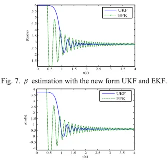
Fig. 6 to Fig. 8 show the filtering results of the unknown
parameters α, β and γrepresented as a parameter vector θ
which are estimated by using the new proposed UKF approach. The filter also can obtain the required parameters and satisfy the anticipated values of GPS observation. And also, UKF make sure the estimation achieve the anticipated values more quickly compare with EKF. Furthermore, compare with Fig. 3 to Fig. 5, it is easy to see that the estimation achievement process to the anticipated values is expedited. Consequently, the computational burden is obviously reduced by using the new proposed UKF. From these figures, the convergence of the new proposed UKF is also verified. 0 10 20 30 40 50 60 70 80 -1 0 1 2 3 4 5 6 t(s) xa (1 00m et er ) UKF EFK sigma points
Fig. 2. The parameter estimation of latitude x ta( ).
0 0.5 1 1.5 2 2.5 3 3.5 4 -1 -0.5 0 0.5 1 1.5 2 2.5 3 t(s) α(ra d/ s) UKF EFK
Fig. 3. The parameter α estimation with UKF and EKF.
0 0.5 1 1.5 2 2.5 3 3.5 4 1.5 2 2.5 3 3.5 4 4.5 5 t(s) β(r ad /s ) UKF EFK
Fig. 4. The parameter β estimation with UKFand EKF.
0 0.5 1 1.5 2 2.5 3 3.5 4 -1 -0.5 0 0.5 1 1.5 2 2.5 t(s) γ(r ad /s ) UKF EFK
Fig. 5. The parameter γ estimation with UKF and EKF.
0 0.5 1 1.5 2 2.5 3 3.5 4 -1 -0.5 0 0.5 1 1.5 2 2.5 3 3.5 4 α(ra d/ s) t(s) UKF EFK
0 0.5 1 1.5 2 2.5 3 3.5 4 1.5 2 2.5 3 3.5 4 4.5 5 5.5 6 t(s) β(ra d/ s) UKF EFK
Fig. 7. β estimation with the new form UKF and EKF.
0 0.5 1 1.5 2 2.5 3 3.5 4 -1 -0.5 0 0.5 1 1.5 2 2.5 3 3.5 4 t(s) γ(ra d/ s) UKF EFK
Fig. 8. γ estimation with the new form UKF and EKF.
The simulations on the vehicle navigation systems with aided GPS in this section verify the proposed algorithm and its performance from the view of experimentation. It is shown that the proposed algorithm has practicability to a certain extent.
6. CONCLUSIONS
Based on the nonlinear filter UKF, the algorithm is presented for linear systems with correlated noises. Fistly, the outline of the problem is presented and the UKF equations are proposed. Then the parameter estimation algorithm is developed and an
extra additive matrix ΔQ is introduced to make sure the
matrices P t( +1)is positive define. Furthermore, the analysis
of the related convergence properties of the algorithm is given. According to some standard results about the convergence of stochastic processes, it is pointed out that, the convergence of the algorithm may be ensured and do not
depend on the magnitude of λ which is an unknown
instrumental diagonal matrix introduced to evaluate the error introduced by linearization. Moreover, the vehicle navigation systems with aided GPS are introduced to show the high performances of the proposed algorithm.
ACKNOWLEGEMENTS
This work is supported by the National Natural Science Foundation of China, under grant 60274009, and Specialized Research Fund for the Doctoral Program of Higher Education, under grant 20020145007.
REFERENCES
Astrom K. J. and P. Eykhoff (1971). System identification -A survey. Automatica, 7, 123-162.
Chin-Lang Tsai and Kao Wei-Wen (2006). Constrained total least-square solution for GPS compass attitude determination. Applied Mathematics and Computation,
183(1), 106-118.
Granados G. Seco and J. A. Ferncindez Rubio (1998). Maximum likelihood propagation-delay estimation in unknown correlated noise using antenna arrays:
application to global navigation satellite systems.
ICASSP '98, 4, 2065-2068.
James L. Garrison and Stephen J. Katzberg (2000). The Application of Reflected GPS Signals to Ocean Remote Sensing. Remote Sensing of Environment, 73(2), 175-187. Jazwinski K. H. (1970). Stochastic Processes and Filtering
Theory. New York: Academic.
Julier S. J., J. K. Uhlmann and H. F. Durrant-Whyte (1995). A new approach for filtering nonlinear systems. Proc. of
the 14th American Control Conference, Seattle,
Washington, 1628-1632. The AACC, Seattle, WA. Julier S. J. and J. K. Uhlmann (1997a). A consistent, debiased
method for converting between polar and Cartesian coordinate systems. The Proc of Aero Sense: 11th Int
Symposium on Aerospace/ Defense Sensing, Simulation and Controls, Orlando, 110-121.
Julier S. J. and J. K. Uhlmann (1997b). A new extension of the Kalman filter to nonlinear systems. The Proc of Aero
Sense: 11th Int Symposium Aerospace/ Defense Sensing, Simulation and Controls, Orlando, 54-65.
Julier, S. J. and J. K. Uhlmann (1997c). A General Method for Approximating Nonlinear Transformations of Probability Distributions [EB/OL]. http:// www. Robots. ox. ac. uk/~siju/ work/ publications/ Unscented. zip, 1997- 09-27.
Julier S. J. (2000). The scaled unscented transformation.
Proceedings of the American Control Conference,
Anchorage, AK, 4555-4559.
Julier S. J., J. K. Uhlmann and H. F. Durrant-Whyte (2000). A new approach for the nonlinear transformation of means and covariances in filters and estimators. IEEE
Trans. on Automatic Control, 45(3), 477-482.
Julier S. J. and J. K. Uhlmann (2004). Unscented filtering and nonlinear estimation. Proceedings of the IEEE, 92(3), 401-422.
Lefebvre T., H. Bruyninckx and J. De Schutter (2002). Comment on ‘a new method for the nonlinear transformation of means and covariances in filters and estimators’. IEEE Trans on Automatic Control, 47(8), 1406-1408.
Ljung L. (1979). Asymptotic behavior of the extended Kalman filter as a parameter estimator for linear systems.
IEEE Trans. on Automatic Control, AC-24(2), 36-50.
Ljung L. (1977). Analysis of recursive stochastic algorithms.
IEEE Trans. on Automatic Control, AC-22(8), 551-575.
Nebot E.M., H. Durrant Whyte and S. Scheding (1998). Frequency domain modeling of aided GPS for vehicle
navigation systems. Robotics and Autonomous
Systems, 25(1-2), 73-82.
Pan Quan, Yang Feng, Ye Liang, Lian Yan and Chen Yong-me. (2005). Survey of a kind of nonlinear filters—UKF.
Control & Decision, 20(5), 481-494 (in Chinese)
Wan E. A. and R. Van Der Merwe (2000). The unscented Kalman filter for nonlinear estimation. Adaptive Systems
for Signal Processing, Communications, and Control Symposium, 153-158.
Xionga K., H. Y. Zhanga and C. W. Chan (2006). Performance evaluation of UKF-based nonlinear filtering.