FIELDS
a dissertation submitted to
the department of physics
and the graduate school of engineering and science
of bilkent university
in partial fulfillment of the requirements
for the degree of
doctor of philosophy
By
Selcen ˙Islamo˘glu
August 2012
Prof. Dr. O˘guz G¨ulseren(Supervisor)
I certify that I have read this thesis and that in my opinion it is fully adequate, in scope and in quality, as a dissertation for the degree of Doctor of Philosophy.
Assoc. Prof. Dr. M. ¨Ozg¨ur Oktel
I certify that I have read this thesis and that in my opinion it is fully adequate, in scope and in quality, as a dissertation for the degree of Doctor of Philosophy.
Asst. Prof. Dr. Co¸skun Kocaba¸s
Prof. Dr. S¸inasi Ellialtıo˘glu
I certify that I have read this thesis and that in my opinion it is fully adequate, in scope and in quality, as a dissertation for the degree of Doctor of Philosophy.
Asst. Prof. Dr. Hande Toffoli ( ¨Ust¨unel)
Approved for the Graduate School of Engineering and Science:
Prof. Dr. Levent Onural Director of the Graduate School
THE INFLUENCE OF EXTERNAL FIELDS
Selcen ˙Islamo˘glu Ph.D. in Physics
Supervisor: Prof. Dr. O˘guz G¨ulseren August 2012
In this thesis, the electronic structure of graphene under the influence of exter-nal fields such as strain or magnetic fields is investigated by using tight-binding method. Firstly, we study graphene for a band gap opening due to uniaxial strain. In contrast to the literature, we find that by considering all the bands (both σ and π bands) in graphene and including the second nearest neighbor interactions, there is no systematic band gap opening as a function of applied strain. Our re-sults correct the previous works on the subject. Secondly, we examine the band structure and Hall conductance of graphene under the influence of perpendicu-lar magnetic field. For graphene, we demonstrate the energy spectrum in the presence of magnetic field (Hofstadter Butterfly) where all orbitals are included. We recover both the usual and the anomalous integer quantum Hall effects de-pending on the proximity of the Dirac points for pure graphene and the usual integer quantum Hall effect for pure square lattice. Then, we explore the evo-lution of electronic properties when imperfections are introduced systematically to the system. We also demonstrate the results for a square lattice which has a distinct position in cold atom experiments. For the energy spectrum of imper-fect graphene and square lattice under magnetic field (Hofstadter Butterflies), we find that impurity atoms with smaller hopping constants result in highly localized states which are decoupled from the rest of the system. The bands associated with these states form close to E = 0 eV line. On the other hand, impurity atoms with higher hopping constants are strongly coupled with the neighboring atoms. These states modify the Hofstadter Butterfly around the minimum and maximum values of the energy and for the case of graphene they form two self similar bands decoupled from the original butterfly. We also show that the bands and gaps due to the impurity states are robust with respect to the second order hopping. For the Hall conductance, in accordance with energy spectra, the local-ized states associated to the smaller hopping constant impurities or vacancies do
not contribute to Hall conduction. However the higher hopping constant impuri-ties are responsible for new extended states which contribute to Hall conduction. Our results for Hall conduction are also robust with respect to the second order interactions.
Keywords: Graphene, tight-binding method, point defects, vacancies, strain, magnetic field, Hofstadter Butterflies, Hall conductance, 2D electronic systems .
GRAFEN˙IN ELEKTRON˙IK YAPISININ DIS
.
ALANLARIN ETK˙IS˙I ALTINDA ˙INCELENMES˙I
Selcen ˙Islamo˘glu Fizik, Doktora
Tez Y¨oneticisi: Prof. Dr. O˘guz G¨ulseren A˘gustos 2012
Bu tezde grafenin elektronik yapısının mekanik gerinim veya manyetik alan gibi dı¸s alanların etkisiyle nasıl de˘gi¸sti˘gi sıkı-ba˘glanım metoduyla incelenmi¸stir.
¨
Oncelikle grafenin tek eksenli gerinim altında enerji bant a¸cıklı˘gı g¨osterip g¨ostermedi˘gini inceledik. Literat¨urden farklı olarak, grafenin b¨ut¨un bant-ları (hem σ hem π bantbant-ları) d¨u¸s¨un¨uld¨u˘g¨unde ve ikincil kom¸su etkile¸simleri hesaba katıldı˘gında grafende uygulanan gerinimin fonksiyonu olarak de˘gi¸sen bir bant a¸cıklı˘gı g¨or¨ulmemektedir. Bizim sonu¸clarımız bu alandaki ¨onceki ¸calı¸smaların sonu¸clarını d¨uzeltmektedir. ˙Ikinci olarak, grafenin bant yapısını ve Hall iletkenli˘gini grafen y¨uzeyine dik manyetik alanın etkisi altında inceledik. Grafenin manyetik alan altındaki enerji bant yapısını (Hofstadter Kelebe˘gi) t¨um orbitaller dahilinde g¨osterdik. Saf grafen i¸cin ola˘gan ve kuraldı¸sı, saf kare a˘g ¨org¨us¨u i¸cin de ola˘gan tamsayı kuantum Hall etkilerini g¨ozlemledik. Daha sonra, elektronik ¨ozelliklerinin sisteme sistematik olarak dahil edilen safsızlıklara g¨ore de˘gi¸simini ¸calı¸stık. Ayrıca, so˘guk atom deneylerinde ¨onemli bir yere sahip olan kristal kare a˘g ¨org¨us¨une ait sonu¸cları da benzer ¸sekilde elde ettik. Kusurlu grafen ve kare a˘g ¨org¨us¨un¨un manyetik alan altındaki enerji tayfı (Hofstadter Kelebek-leri) i¸cin, k¨u¸c¨uk sekme katsayısına sahip kusurlar, y¨uksek oranda yerel olarak konumlanmı¸s ve sistemin geri kalanından ayrılmı¸s ¨oz-de˘gerlik durumlarına sebe-biyet vermektedir. Bu durumlarla ili¸skili bantlar E = 0 eV ¸cizgisine yakın olarak bi¸cimlenmi¸stir. Di˘ger taraftan, b¨uy¨uk sekme katsayısına sahip kusurlar ise kom¸su atomlarla y¨uksek oranda ba˘gla¸sıma girmi¸slerdir. Bu ¨oz-de˘gerlik durumları Hofs-tadter Kelebekleri’ni enerji de˘gerlerinin en k¨u¸c¨uk ve en b¨uy¨uk oldu˘gu b¨olgelerde de˘gi¸sikli˘ge u˘gratmakta ve grafen s¨oz konusu oldu˘gunda ¨ozg¨un kelebekten tama-men ayrılmı¸s iki adet ¨oz-benze¸s bant olu¸sturmaktadır. Ancak, kusur ¨oz-de˘gerlik durumları nedeniyle olu¸san bantlar ve bant a¸cıklıkları ikinci derece sekmeye kar¸sı diren¸clidir. Hall iletkenli˘gi i¸cin de, enerji tayfındaki de˘gi¸sikliklerle uyumlu olarak,
k¨u¸c¨uk sekme katsayısına sahip kusur ve bo¸sluklar k¨okenli y¨uksek oranda yerel olarak konumlanmı¸s ¨oz-de˘gerlik durumlarının Hall iletkenli˘gine katkıda bulun-madıkları soylenebilir. Fakat, g¨orece b¨uy¨uk sekme katsayısına sahip kusur atom-ları Hall iletkenli˘gine katkıda bulunan yersizle¸smi¸s yeni ¨oz-de˘gerlik durumatom-larının olu¸smasına neden olmaktadır. Hall iletkenli˘gi hesaplarımızın sonu¸cları da ikinci derece etkile¸simler kar¸sında kalıcıdır.
Anahtar s¨ozc¨ukler : Grafen, sıkı-ba˘glanım metodu, noktasal kusurlar, eksiklik-ler, gerinim, manyetik alan, Hofstadter Kelebekleri, Hall iletkenli˘gi, ˙Iki boyutlu elektronik sistemler .
This dissertation would not have been accomplished without the help, support and guidance of several individuals who in some way contributed and offered their valuable assistance during the preparation of this study.
First and foremost, my utmost gratitude to Prof. Dr. O˘guz G¨ulseren, whose sincerity, help, motivation and encouragement I am very much indebt to. I also would like to thank Assoc. Prof. Dr. M. ¨Ozg¨ur Oktel for his priceless and endless contributions, suggestions and support,
Our group members: Dr. G¨ursoy Bozkurt Akg¨u¸c and H¨useyin S¸ener S¸en for the insight they share and for the moral support. In addition, our former group member Dr. Rasim Volga Ovalı who has been and always will be a real and “robust” friend of mine for the rest of my life; my office-mate and dear friend
¨
Umit Kele¸s, for his friendship, in-office lunches, “verba volant scripta manent”, and valuable conversations and discussions; “girls”: Mrs. Hatice Yılmaz, Mrs. Elvan ¨O˘g¨un and Mrs. Gizem Erkilet for the coffee breaks, risotto nights and for being such nice real friends; my all other dear friends who once were members of this department or the university; Dr. Sevilay Sevin¸cli, Dr. Haldun Sevin¸cli, Musa Kurtulu¸s Abak, ˙Imran Avcı and Dr. M. Emre Ta¸sgın for always being here for me, and all the staff of the Physics Department;
My dear great family: My mothers G¨ulfem Aydemir and Sevim ˙Islamo˘glu,
my fathers H. Baki Aytekin and Erdal ˙Islamo˘glu, my brother Ali Y. Aytekin and my sister Sezin Kadıo˘glu, without whom I can not imagine an alternative life, for always supporting me with endless patience; my son Badem for never leaving me alone and obstinately sleeping on my papers and stuff when I study;
Lastly, I would like to thank to my love, my husband, my best friend H. Erol ˙Islamo˘glu, before whom my heart was lost on a distant planet, for all the colors he brought to my life and for supplying me strength not to throw in the towel.
1 Introduction 1
2 The Tight-Binding Method 5
2.1 The Tight-Binding Approximation—Overview . . . 5
2.2 Tight-Binding Method for Mono-layer Graphene . . . 8
2.3 Calculation of the Fermi Level . . . 12
2.4 Imperfections in 2D Electronic Systems . . . 13
3 Electronic Structure of Graphene under Uniaxial Strain 14 3.1 Tight-Binding Method under the influence of Uniaxial Strain . . 14
3.2 Energy Spectrum of Strained Graphene . . . 16
3.2.1 Energy-Band Structure of Strained Graphene . . . 18
4 Hofstadter Butterflies of Square Lattice and Defective Square Lattice 36 4.1 Energy Spectrum Under the Influence of Perpendicular Magnetic Field . . . 36
4.1.1 Square Lattice with a Single Atom in the Basis . . . 37
4.2 Defective Square Lattice . . . 40
4.2.1 Enlarged Unit Cell . . . 42
4.2.2 Square Lattice of 9 Atoms in the Basis . . . 48
4.3 Hofstadter Butterflies of Defective Square Lattice . . . 51
5 Hofstadter Butterflies of Graphene and Defective Graphene 54 5.1 Graphene in Perpendicular Magnetic Field . . . 54
5.2 Defective Graphene . . . 59
5.2.1 Enlarged Unit Cell of Graphene . . . 61
5.3 Hofstadter Butterflies of Defective Graphene . . . 65
5.3.1 First Nearest Neighbors . . . 66
5.3.2 First and Second Nearest Neighbors . . . 69
5.3.3 Impurity States . . . 69
6 Hall Conductances for Defective Square Lattice and Graphene 75 6.1 Integer Quantum Hall Effect . . . 75
6.2 Topology in Hall Conductance . . . 78
6.3 Hall Conductances for Defective Square Lattice . . . 81
6.4 Hall Conductances for Defective Graphene . . . 86
6.4.1 Anomalous Integer Quantum Hall Effect in Graphene . . . 86
2.1 Graphene in real and reciprocal space. . . 9
2.2 Orbital orientations. . . 10
2.3 Band diagram of graphene. . . 11
3.1 Graphene under strain. . . 15
3.2 Energy-band diagram of graphene with 1st nearest neighbors tight-binding method under 25% strain applied with θ = 300 with Pois-son’s ratio σ = −0.165 and the decay rates were scaled with expo-nential scaling to be the same for all directions. . . 20
3.3 Energy-band diagram of graphene with 1st and the 2nd nearest neighbors tight-binding method under 30% strain applied with θ = 300with Poisson’s ratio σ = −0.165 and the decay rates were scaled with exponential scaling to be the same for all directions. . . 21
3.4 Poisson’s ratio versus energy-band gap for θ = 00, with exponential scaling and same hopping constants (decay rates) for all directions for the 1st nearest neighbors. . . . . 22
3.5 Poisson’s ratio versus energy-band gap for θ = 00, with exponen-tial scaling and different hopping constants (decay rates) for all directions for the 1st nearest neighbors. . . . . 23
3.6 Poisson’s ratio versus energy-band gap for θ = 300, with
expo-nential scaling and same hopping constants (decay rates) for all directions for the 1st nearest neighbors. . . . . 24
3.7 Poisson’s ratio versus energy-band gap for θ = 300, with
exponen-tial scaling and different hopping constants (decay rates) for all directions for the 1st nearest neighbors. . . . . 25
3.8 Poisson’s ratio versus energy-band gap for θ = 600, with
expo-nential scaling and same hopping constants (decay rates) for all directions for the 1st nearest neighbors. . . . . 26
3.9 Poisson’s ratio versus energy-band gap for θ = 600, with
exponen-tial scaling and different hopping constants (decay rates) for all directions for the 1st nearest neighbors. . . . . 27
3.10 Strain versus energy-band gap for σ = 0.300, with exponential scal-ing and different hoppscal-ing constants (decay rates) for all directions for the 1st nearest neighbors tabulated for several angles. . . . . 28
3.11 Strain versus energy-band gap for σ = 0.300, with exponential scaling and same hopping constants (decay rates) for all directions for the 1st nearest neighbors tabulated for several angles. . . . . 29
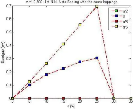
3.12 Strain versus energy-band gap for σ = −0.300, with exponential scaling and different hopping constants (decay rates) for all direc-tions for the 1st nearest neighbors tabulated for several angles. . 30
3.13 Strain versus energy-band gap for σ = −0.300, with exponential scaling and same hopping constants (decay rates) for all directions for the 1st nearest neighbors tabulated for several angles. . . . . 31
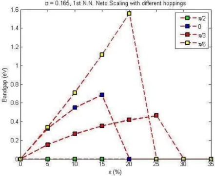
3.14 Strain versus energy-band gap for σ = 0.165, with exponential scal-ing and different hoppscal-ing constants (decay rates) for all directions for the 1st nearest neighbors tabulated for several angles. . . . . 32
3.15 Strain versus energy-band gap for σ = 0.165, with exponential scaling and same hopping constants (decay rates) for all directions
for the 1st nearest neighbors tabulated for several angles. . . . . 33
3.16 Strain versus energy-band gap for σ = −0.165, with exponential scaling and different hopping constants (decay rates) for all direc-tions for the 1st nearest neighbors tabulated for several angles. . 34
3.17 Strain versus energy-band gap for σ = −0.165, with exponential scaling and same hopping constants (decay rates) for all directions for the 1st nearest neighbors tabulated for several angles. . . . . 35
4.1 Square lattice. . . 37
4.2 Magnetic unit cell of the square lattice. . . 38
4.3 Hofstadter Butterfly for square lattice. . . 39
4.4 Square lattice unit cell configurations . . . 41
4.5 Organization scheme for Am matrix. . . 45
4.6 Magnetic unit cell of enlarged square lattice. . . 48
4.7 Hofstadter Butterflies for impure square lattice with the 1st order interactions . . . 49
4.8 Hofstadter Butterflies for impure square lattice with the 1st and 2nd order interactions . . . . 50
4.9 Wavefunctions of localized states. . . 51
5.1 Enlarged unit cell of graphene with 4 atoms. . . 55
5.2 Hofstadter Butterfly for graphene, only pz orbitals are considered. 58 5.3 Hofstadter Butterfly for graphene, all orbits are included. . . 60
5.4 Enlarged unit cell of graphene with 8 atoms. . . 62 5.5 Hofstadter Butterflies for impure graphene with the 1st order
in-teractions . . . 67
5.6 Hofstadter Butterflies for impure graphene with the 1st and 2nd
order interactions . . . 70
5.7 Probabilities of wavefunctions as a function of impurity hopping
strengths. . . 71
5.8 Band evolution as a function of impurity hopping strengths. . . . 72
6.1 Hall conductivities for impure square lattice with the 1st order
interactions. . . 82 6.2 Hall conductivities for impure square lattice with the 1st and 2nd
order interactions. . . 83
6.3 Enlarged magnetic unit cells of graphene . . . 88
6.4 IQHE and anomalous IQHE of graphene. . . 91
6.5 Hall conductivities for impure graphene with the 1st order
interac-tions. . . 93 6.6 Hall conductivities for impure graphene with the 1st and 2nd order
interactions. . . 94
6.7 Hofstadter Butterflies with Hall conductances for graphene. . . 98
2.1 Tight-binding interaction parameters for graphene . . . 11
4.1 The scheme for the interactions between the atoms. . . 46
Introduction
Carbon is the basic element of Nature. Various structures having carbon atoms have been popular fields of research through the last few decades. Among these systems, two dimensional (2D) graphene, composed of only carbon atoms, has a basic and a unique position in order to examine the other carbon-based systems [1]. It became experimentally accessible after the isolation as single layer by me-chanical exfoliation [2, 3]. As a result, it is one of the systems that attracted the most attention in recent years. There are several works that concentrate on the electronic and mechanical properties of graphene [4, 5, 6, 7]. The band struc-ture of graphene was determined in 1947 [8]. Graphene exhibits several unusual properties because of the Dirac points appearing in its band structure. The π
bands due to the pz orbitals of graphene form conic shapes and the conduction
and valance bands touch each other at Dirac points. These bands of graphene are unique in 2D electronic systems, where the relativistic quantum mechanics gov-erns the system due to the linear dispersion of Dirac cones. The behavior of Dirac fermions under magnetic fields and electrostatic potentials is a popular interest for researchers [4, 5, 9, 10, 11, 12]. One of the main consequence of graphene’s band structure is the observation of anomalous integer quantum Hall effect in low magnetic fields which was predicted by earlier calculations [12, 13]. Soon after the discovery of the anomalous integer quantum Hall effect in graphene [5, 14], many theoretical studies discussing the Hall conductance in low magnetic field
regime were reported [15, 16, 17, 18, 19].
One of the most popular questions asked by researchers is whether it is pos-sible to apply band gap engineering on graphene. To investigate this point, the effects of uniaxial strain on graphene’s band structure has been determined theo-retically as well as experimentally [20, 21, 22, 23, 24, 25, 26]. The most interesting result was reported by Castro-Neto et al. which indicated that it is possible to obtain a band gap opening in graphene by applying ∼ 24 % uniaxial strain due to the merging of the Dirac cones [27, 28]. They have used the nearest neighbor tight-binding method which is a very practical approach and it is capable of in-vestigating the electronic structure in a smart way. The analytical tight-binding method applied to graphene was published in 2002 [29]. However, in that pa-per, the only bonds under consideration were the π bonds, and the calculation contained only the 1st nearest neighbors, since this level of approximation was
thought to provide information about the one-dimensional nanotube band struc-ture. Since the band structure of graphene is not composed of only π bonds, we provide a detailed calculation about the band structure which contains σ bonds as well as the π bonds.
The effects of the external field induced changes on the electronic structure of graphene is a very interesting and promising problem. In this thesis, we concen-trate on two external fields: strain and magnetic field which can be investigated
by the tight-binding method. Firstly, we demonstrate the results of 2nd
near-est neighbor tight-binding approach applied to single-layer graphene under strain which has an opposing result to what was reported in the literature. Another re-cent study suggests that, with 26.5% of uniaxial strain the system develops a 45.5 meV band gap [30]. We claim that, it is impossible to get a band gap opening in monolayer graphene by applying uniaxial strain. Secondly, we examine graphene and a square lattice which is also a 2D system under magnetic field. The choice of the square lattice is due to its simple yet representative nature. Moreover it also has a unique position in cold atom experiments and calculations [31, 32, 33, 34]. We use tight-binding method again up to second order interactions through which we obtain the energy spectra under magnetic field (Hofstadter Butterflies) and
the Hall conductance values. In addition we demonstrate the effects of lattice im-perfections on the electronic structure when the system is subjected to magnetic field.
Graphene is composed of a layer of hexagonally arranged carbon atoms, which has a structure similar to honeycomb. It is a sp2 hybridized structure, in which
the hybridization of one s orbital with two p orbitals (px and py) leads to the
formation of σ bonds among the carbon atoms. As a result of this, graphene has
a trigonal planar geometry with carbon atoms which are separated by 1.42 ˚A.
The remaining p orbital (pz) which is perpendicular to the plane of consideration,
is responsible for the covalent bonding to upper or lower layer neighboring atoms which has a consequence of the formation of π bonds. In this thesis, we mostly concentrated on the electronic structure due to π bonds which are the leading features for magnetic field considerations, however for the case of strain the σ bonds have an important role.
In 2D, the Bloch electrons display an unusual behavior under magnetic field. When there is a perpendicular magnetic field applied to the system the spectrum has a fractal structure which depends on the magnetic flux, the chemical potential and the temperature. The fractal nature of this spectrum originates from two different length scales competing with each other: The length scale of the unit cell which is governed by the lattice constant and the magnetic length of the system. This competition gives rise to the phenomenon called “frustration” [35]. This unique spectrum is actually a phase diagram of the system with infinitely many phases. The spectrum consist of recursive subbands which form phase boundaries around the gaps. This structure of bands and gaps is generated by the adiabatic changes in the magnetic flux and the chemical potential. The number of subbands is dependent on some number connected to the magnitude of the magnetic field. Hypothetically, this number “q” can be represented as a function of the fraction of magnetic flux per plaquette penetrating into the system to flux quanta. This ratio actually is the ratio of two characteristic periods of the system: period of a single electron in a state with crystal momentum 2π¯h/a, “a” is being simply the lattice constant and the other period is the reciprocal of the cyclotron frequency [36]. The energy spectrum of these electrons display a
self-similar structure. The primary work was performed by Douglas R. Hofstadter in 1976, which concentrates on the square lattice and later these unique spectra have been called by his name: The Hofstadter Butterflies [36] for several 2D electronic systems. Several works concentrated on the energy spectra of various examples of the 2D lattices, such as square, triangular, hexagonal, and honeycomb lattices [37, 38, 39, 40, 41, 42, 43]. Although graphene is a non-Bravais lattice, with two atoms in its basis, it still represents a fractal energy spectrum under magnetic field.
The Hofstadter Butterfly has another interesting property. It gives informa-tion about the magnetotransport properties of the system. Each gap in the energy spectrum has a certain Hall conductance value within a gap. These values are associated to every gaps and they stay constant within the gaps. These constant values of Hall conductance indeed correspond to the Hall conductance plateaus when the conductance is plotted as a function of Fermi Energy. The conductance values of the gaps can be determined by the Diophantine equation whose solu-tions are known as Chern numbers [44] for the square and honeycomb lattices as long as the Fermi energy or the chemical potential lies in a gap. The relation between the Hall conductance and the Chern numbers originates from the topo-logical aspects of the Hall conductance. However, since the Diophantine equation is no longer valid when there are imperfections in the system, we use a general Kubo formula for Hall conductance calculation which gives results regardless of the position of the Fermi energy.
The thesis is organized as follows: In the first chapter, we demonstrate the general methodologies that we used in our calculations. Then, we concentrate on the electronic behaviors of graphene under two external fields: Strain and perpendicular magnetic field. For the magnetic field, we also studied the square lattice. Moreover, we monitor the changes on the energy spectra and the Hall conductance as a function of imperfections introduced to the systems periodically for both graphene and the square lattice.
The Tight-Binding Method
2.1
The Tight-Binding Approximation—Overview
Tight-binding approximation -also referred to as Linear Combination of Atomic Orbitals (LCAO)- is one of the simplest tools for calculating band structures. In this method, the orbitals which are based on atomic states are used as a basis for the expansion of the crystal wavefunction. Since the crystal wavefunctions are tightly bound to the atoms, the name “tight-binding” was given for this method. Suppose that the orbital set φl(r − ti) is centered at the position of the ith
atom, denotes the set of atomic wavefunctions where ti is the position of the ith
atom and l is one of the angular momentum characters such as s, p, d and etc. Then, we can use this set of wavefunctions as a basis for expanding the crystal wavefunctions {χkli(r)} which obey the Bloch’s theorem:
χkli(r) = 1 √ N X R′ eik·R′φl(r − ti − R′) , (2.1)
N is the number of unit cells in the crystal,
χkli(r + R) = 1 √ N X R′ eik·R′φl(r + R − ti − R′) = √1 N X R′ eik·(R′−R)eik·Rφl(r + R − ti − R′) = eik·R 1√ N X R′ eik·(R′−R)φl(r − ti − (R′− R)) = eik·R 1√ N X R′′ eik·R′′φl(r − ti − R′′) = eik·Rχkli(r), (2.2)
and R′′ = R′− R is just another lattice vector. The single particle eigenstates can be expanded via these functions as follows:
ψk =(n) X i,l
c(kil(r)χkn) li(r). (2.3)
Under these circumstances the single particle Schr¨odinger equation now becomes:
Hspψnk(r) = ǫkψk(r);n X i,l[hχkmj |Hsp|χklii − ǫ (n) k hχkmj|χklii]c (n) kli = 0 (2.4)
Now, we have two sets of integrals to deal with. The first one hχkmj|χklii are
“overlap matrix elements” which can be defined as follows hχkmj|χklii = 1 N X R′ ,R′′ eik·(R−R′′)hφm(r − tj − R′′)|φl(r − ti− R′)i = 1 N X R,R′ eik·Rhφm(r − tj)|φl(r − ti− R′)i = X R eik·Rhφ m(r − tj)|φl(r − ti− R)i
The 1/N factor drops out since there is no more explicit dependence on R′ owing to crystal symmetry. In a similar manner one can calculate the second integral
hχkmj|H sp |χklii; hχkmj|H sp |χklii = X R eik·Rhφm(r − tj)|Hsp|φl(r − ti− R)i (2.5)
One of the main approximations behind the tight-binding theory is “the or-thogonal basis approximation”, which approximates by a diagonal one i.e. the overlap matrix (represented by S), elements to be nonzero if and only if they are acting for the same orbitals on the same atom such that;
hφm(r − tj)|φl(r − ti − R)i = δlmδijδ(R) . (2.6)
In fact this is just a useful assumption, since if the overlap matrix elements were to be strictly zero for different orbitals, then we would have no interactions among the nearest neighbors. For the Hamiltonian matrix elements we have a similar situation, if they are acting for the same orbitals on the same atom we get the “on-site” energies:
hφm(r − tj)|Hsp|φl(r − ti− R)i = δlmδijδ(R)ǫl (2.7)
If the orbitals are on different atoms but these atoms are located at the nearest neighbor sites which are represented by vector dnn;
hφm(r − tj)|Hsp|φl(r − ti− R)i = δ((tj − ti− R) − dnn)Vlm,ij (2.8)
we obtain the Vlm,ij “hopping matrix elements”. The on-site energies and the
hopping matrix elements and the overlap matrix elements are parameterized and tabulated [45, 46].
For generalized tight-binding method, the off-diagonal elements of the overlap matrix S are not necessarily non zero. In the presence of non zero values for overlap matrix elements, the energy eigenvalues are the solutions of:
det(H − SE) = 0 .
However, this equation can be reduced to orthogonal tight-binding method:
by L¨owdin transformation. In our tight-binding calculations our parameter are modified in accordance with the generalized tight-binding, however we solve Eq. 2.9.
2.2
Tight-Binding Method for Mono-layer Graphene
Graphene has a hexagonal lattice structure which can be constructed by two lattice vectors, ~ a1 = a√3 2 x +ˆ a 2yˆ (2.10) ~ a2 = a√3 2 x −ˆ a 2yˆ (2.11)
where a is the distance between the carbon atoms. The reciprocal lattice vectors can be calculated from the basis vectors. In addition, graphene has two identical atoms in its basis, which are labeled as atoms type A and type B, as shown in Figure 2.1.
According to the tight-binding method, the Hilbert space which is spanned by the atomic-like orbitals is able to describe the wavefunction solutions of the Schr¨odinger equation [45]. These wavefunctions satisfy Bloch’s Theorem due to the translational symmetry. Under these circumstances, the tight binding Hamil-tonian for graphene can be written as an 8×8 matrix, including the interactions of one s and three p orbitals. A convenient way to visualize this matrix is writing it as a composite of four blocks according to the consideration of atoms A and B.
H = HAA HAB HBA HBB , (2.12)
Each of HAA, HAB, HBA, and HBB are 4×4 matrices denoting the orbital
interactions of atom A with itself, atom A and atoms B, atom B atoms A, and atom B with itself, respectively. The eigenvalues of this Hamiltonian give the desired energy values. In our calculations, we did not take the overlap matrix into account, since its already implemented through the parameter we use. For more
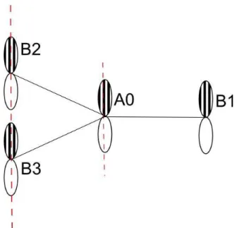
A0 A1 A2 A3 A5 A4 A6 B2 B1 B3 a1 a2
M
K
Γ
M'
K'
b1
b2
kx
ky
Figure 2.1: Graphene in real and reciprocal space. The nearest neighbors of atom A0 up to 2nd order are presented in the first picture. The high symmetry points
used in the construction of a route in drawing the band structure are shown in the second figure.
accurate energy values, instead we took our calculations two steps further via inclusion of px and py orbitals and also the second nearest neighbor interactions
into the calculations in comparison to the similar work done before [27]. As an example to the components of the main Hamiltonian matrix given in equation
2.12, HAA and HAB are displayed below.
HAA = h2SA|H|2SAi h2SA|H|2PA xi h2SA|H|2PyAi h2SA|H|2PzAi h2PA x |H|2SAi h2PxA|H|2PxAi h2PxA|H|2PyAi h2PxA|H|2PzAi h2PA y |H|2SAi h2PyA|H|2PxAi h2PyA|H|2PyAi h2PyA|H|2PzAi h2PzA|H|2SAi h2PzA|H|2PxAi h2PzA|H|2PyAi h2PzA|H|2PzAi HAB = h2SA|H|2SBi h2SA|H|2PB x i h2SA|H|2PyBi h2SA|H|2PzBi h2PA x |H|2SBi h2PxA|H|2PxBi h2PxA|H|2PyBi h2PxA|H|2PzBi h2PA y |H|2SBi h2PyA|H|2PxBi h2PyA|H|2PyBi h2PyA|H|2PzBi h2PA z |H|2SBi h2PzA|H|2PxBi h2PzA|H|2PyBi h2PzA|H|2PzBi
Figure 2.2: The orientations of py orbitals for nearest neighbor atoms A0, B1,
B2, and B3
When there is no strain in the system, h2PA
y |H|2PyBi can be thought as a
sum of h2PA0
y |H|2PyB1i, h2PyA0|H|2PyB2i, and h2PyA0|H|2PyB3i, since atom type
A labeled as “A0” in Figure 2.1 has only three nearest neighbors of atom type B. Since the px and py orbitals are oriented with some angle (α) with respect
to each other due to the structure of the lattice as sketched in Figure 2.2, the individual matrix elements should be calculated by decomposing the orbitals into
σ and π components. As an example the matrix element h2PA
y |H|2PyBi can be
decomposed as follows:
h2P yA0|H|2P yB1i = (−V
ppσcos2α1+ Vppπsin2α1)ei~k·~b1
h2P yA0|H|2P yB2i = (−Vppσcos2α2+ Vppπsin2α2)ei~k·~b2
h2P yA0|H|2P yB3i = Vppπei~k·~b3 , (2.13)
where, Vppσ and Vppπ are the interaction parameters between the σ and π
or-bitals, respectively, and ~b1 and ~b2 are the reciprocal lattice vectors. The general
expressions for these interactions can be found in the References [45, 47]. The energy-band diagram of graphene can be viewed via Fig. 2.3, where all the orbitals are considered. We use the parameter set given in Table 2.1 for graphene.
−30 −25 −20 −15 −10 −5 0 5 10 En e rg y(e V) ε = 0, θ = 0, σ = 0.165 Γ M‘ K‘ K Γ M K
Figure 2.3: The energy-band diagram of graphene when all the orbitals are taken into account.
Nearest neighbour Next nearest neighbour
On-site interaction interaction
energies parameters parameters
ǫ2s -7.3 Vss -4.30 Vss2 -0.18
ǫ2p 0.0 Vsp 4.98 Vsp2 0.0
Vppσ 6.38 Vppσ2 0.35
Vppπ -2.66 Vppπ2 -0.10
Table 2.1: Tight–binding interaction parameters for graphene from Ref. [46]. All values are in eV. ǫ2s and ǫ2p are the self interactions of the s orbital and the
p orbitals. Vss and Vsp are the interactions of s orbital with the neighboring s
orbital, s orbital with the neighboring p orbital, respectively. Vppσ and Vppπ are
2.3
Calculation of the Fermi Level
In order to determine whether there is a band gap or not, one should be able to calculate the Fermi level. Fermi level is defined as the energy of the topmost filled level in the ground state of the N electron system [50]. For the most general case, we can define a density of levels per unit volume g(ε) so that the general expression for a variable q can be written as:
q =
Z
dεg(ε)Q(ε) (2.14)
where, q can be defined for two separate cases. If q is the electronic number density n, then Q(ε) = f (ε), where f (ε) is the Fermi Dirac distribution function; if q is the electronic energy density u, then Q(ε) = εf (ε) [51]. The density of states (or levels) can be easily obtained from the band diagram. However, for this purpose the selection of the k points requires great importance. Rather than calculating the band diagram through a certain route composed of high symmetry points in the reciprocal lattice, one should sample all the k points located in the 1st Brillouin zone. The details about the sampling of the Brillouin zone can be
found in Ref. [52]. After the calculation of the band diagram, the DOS (density of states) information can be obtained basically via the consideration of the number of states per unit volume and per unit energy window. With the number of electrons fixed at n and the assumption that the system is at 0 K, the equation 2.14 reduces to :
Z Ef
−∞D(ε)dε = n, (2.15)
with Ef is the Fermi level, since for 0 K f (ε) is 1. The integration limits originate
from the definition of the Fermi level. This numerical integral can be performed iteratively, and as a result the value for the Fermi level can be estimated, easily. In the band diagrams represented throughout the remaining pages, the Fermi level is set to 0 eV.
2.4
Imperfections in 2D Electronic Systems
The imperfections can be natural parts of solid state systems formed accidentally as well as ingredients introduced in the cold atomic systems intentionally by re-designing the optical lattice or by including several atomic species as in recent experiments [81, 82, 83]. We model both the square lattice and graphene with impurities to observe the changes in their magneto-transport properties under the influence of perpendicular magnetic field. The tight-binding method which is a sufficient tool both for the calculation of the energy spectrum (Hofstadter Butterflies) as a function of magnetic flux φ divided by flux quantum φ0 and the
Hall conductance still serves well for the systems with impurities. The method-ology is the same as with the one outlined in the previous sections except for some points. First, we define the imperfections as impurity atoms replaced by the original atoms of the basis and vacancies where there exists no atoms. These considerations bring regulations in the hopping parameters. For impurity atoms we simply change the first and the second nearest neighbor hopping parameter of the imperfection, and for the vacancy case they simply become 0. The second difference from the pure cases is that in order to achieve reasonable concentra-tions of impurities by forbidding the system to become an alloy, we enlarge the unitcell. By doing this we are able to work with systems which have arrays of imperfections distributed periodically as imperfection lattices over the remaining lattices. However since the system size is enlarged the calculation cost increases. The size of the Hamiltonian in the magnetic field increases in accordance with the number of atoms considered.
Electronic Structure of Graphene
under Uniaxial Strain
3.1
Tight-Binding Method under the influence
of Uniaxial Strain
Since graphene has many independent electronic and mechanical properties which attract the interest of scientists around the world, an investigation into the unified electro-mechanical properties is of great interest. There have been many inves-tigations about the mechanical properties such as elasticity [23] and resistance to elastic deformations both by ab-initio calculations and several experiments [21, 48]. In addition, the effects of strain were observed via the Raman Spectra, where with the application of strain the Raman peaks shift and may even be split into sub-peaks [20].
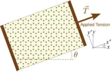
In our calculations, we concentrated on the effects of the uniaxial strain on the band diagram of mono-layer graphene. A simple sketch (Figure 3.1) for this was published in Reference [27]. In order to implement the strain information into the calculations, we first developed an algorithm for the change in the positions of the atoms with respect to the applied strain. This geometric algorithm contains
Figure 3.1: The schematic view of strain applied to graphene. The picture is taken from V. M. Pereira, A.H. Castro Neto, N.M. Peres, arXiv: 0811.4396v3 [cond-mat.mtrl-sci], 2009 (Ref. [27]).
the information of the amount of the strain and also the direction through the strain was applied. This re-scaling process basically depends on the change in the vectors under applied strain. The generalization of this fact can be done by considering a general vector ~υ0 which is not initially under strain. This vector ~υ0
transforms into a new vector ~υ with the applied strain by: ~υ = (¯1 + ¯ε) · ~υ0
¯ ε = ǫ
cos2θ − σ sin2θ (1 + σ) cos θ sin θ
(1 + σ) cos θ sin θ sin2θ − σ cos2θ
, (3.1)
where ¯1 is the unit matrix, ¯ε is the strain tensor, ǫ is the amount of strain which is just a ratio of amount of elongation or compression divided by the initial length (ǫ being positive or negative, respectively), σ is Poisson’s ratio, and θ is the angle between the plane of the atoms and the applied strain. All the vectors in the system were subjected to this strain transformation. Within this formulation strain has a first order effect on the bond lengths and the atomic distances. However, when we look at the interaction parameters between the orbitals, we can claim that strain has a second order influence on these parameters. In order to scale, we simply used two transformations, one is an exponential scaling given Ref. [27], and the other is simply square scaling;
Vppσnew = Vppσe−β( l a0−1), (3.2) Vnew ppσ = Vppσ( l a0 )2, (3.3)
where l is the new bond length, a0 is the initial one, β is the scaling parameter
and decay rate extracted from the experimental results [49].
3.2
Energy Spectrum of Strained Graphene
When we consider graphene without strain it is easy to calculate the energy bands from tight-binding Hamiltonian. However when there is stress applied to system, the main Hamiltonian should be reconstructed in order to implement this stress information into the calculation. The easiest way to introduce stress to a system is
modifying the Hamiltonian and lattice parameter with strain. Strain is a unitless measure of stress, it is the amount of elongation or compression divided by the initial length. It changes sign due to being an elongation or compression strain. There are several consequences of uniaxial strain applied to a (2D) system:
• Due to the strain, all the vectoral quantities in the real space, including the primitive lattice vectors, the distance between the atoms should be re-arranged by the strain tensor as shown in Eq. 3.1. The atoms change their initial positions, and the bond-distances change as a result of that. Since the strain uniform and uniaxial, and we are studying the bulk electronic properties, the lattice vectors should also be modified to expand the calcu-lations among the infinite surface.
• As a result of changes in real space, all the vectors and distances in the reciprocal space should be modified, too. Similarly, the reciprocal lattice vectors, the coordinates of high symmetry points are all altered due to strain.
• Due to the contraction or elongation in the atomic distances, the inter-action parameter must be subject to a scaling algorithm. The main scaling types are already given in Eq. 3.2 and Eq. 3.3.
• Due to the change of the positions of the atoms, the orientations of the atomic orbitals with respect to each other are also modified. The angles between the orbitals should be subjected to modifications as a function of strain.
In our analysis, we used the tight-binding method with the first and the also with the second order interactions. We also tested both the square scaling the exponential scaling of the orbital interaction parameter. We also considered the isotropic case, where the orbital interaction parameter are the same for all bond directions. In addition to that, we also studied the anisotropic case in which the orbital interaction parameter are different among the different bond directions.
The main calculations for this chapter involves the sets of parameter itemized below:
• Several strain values; “ǫ” the amount of strain percentage is scanned for 0, 5, 10, 15, 20, 25, 30 and 35 %.
• Different Poisson’s ratios “σ” were used: −0.300, −0.250, −0.200, −0.180, −0.170, −0.165, −0.160, −0.150, −0.140, −0.130, −0.120, −0.110, −0.100, −0.05, 0, and 0.300, 0.250, 0.200, 0.180, 0.170, 0.165, 0.160, 0.150, 0.140, 0.130, 0.120, 0.110, 0.100, 0.05.
• And also several angles through which strain is applied to the plane of graphene: 0, π/2, π/3, π/6, π/12, 9π/180, 17π/180, 23π/180.
3.2.1
Energy-Band Structure of Strained Graphene
As it is mentioned in section 3.1, we introduced uniaxial strain to the system. According to this information, all the vectoral quantities are transformed. When plotting the band diagram we also modified the coordinates of the high sym-metry points and the distance between them which comes automatically as a consequence of the change in the coordinates. Secondly, due to change in the inter-atomic distances, the interaction parameter are also rescaled. There are two main scaling methods, one is exponential scaling, the other one is square scaling for which the explicit representations were given in Equations 3.2 and 3.3. We tested both of them. And also we tried two different conditions, one the scaling functions differ for each directions by the change of one variable β, and for the second condition we considered it to be the same for the all directions which corresponds to the isotropic case. In Ref. [1] β is reported to be 3, 3.14, and 4.
The angle θ which represents the angle of strain direction to the graphene surface, corresponds to 0 degrees for the armchair direction and the horizontal axis coincides with the armchair direction. We scanned the reported values for θ, the symmetric angles for graphene as well as some values for the chiral angles.
For the case of choice for the value of the Poisson’s ratio σ, we performed a wide range of calculation between the values −0.300 and 0.300 since there is no strict information about the ratio for mono-layer graphene reported in the literature. The most common value for σ is 0.165 [84] but it is stated that this is the measured value for graphite [1, 85]. However, many researchers are using this value in their calculations. Also there is another reported range for graphene’s Poisson’s ratio which is said to be lie in between 0.10 and 0.14 [86]. In order to convince ourselves, we tested a wide range for the parameter.
Since we try to obtain a band gap opening as a result of strain, we test graphene for the strain amounts between 0 to 35 % through which the graphene is able to stay unbuckled.
The last point we concentrated on is to preserve the lattice structure through applying strain in the chiral angles, since the lattice may not be defined anymore. To check this condition, we defined chiral and translational vectors corresponding to the desired values for angles in other words for the pairs (m, n) commonly used by researchers working on nanotubes. For a net to define a lattice, these vectors should be perpendicular to each other. With the effect of strain these vectors change as well, but they should still be perpendicular to each other. We have written an algorithm which keeps the track of this information. It came out that in none of our calculations we are losing the lattice.
For the basic angles 0, 30, 60 and 90 degrees we obtain the following results: There is a band gap between 10 and 25% of strains for 30 and 60 degrees, as shown in Fig. 3.2. When the amount of strain is increased to 30%, the conduction and valance bands intersect the Fermi level which can be viewed via Fig. 3.3 . And this behavior is similar for all the Poisson’s ratio in the neighborhood of 0.165
and −0.165 when 1st nearest neighbors are considered and the scaling scheme
chosen to be as exponential. When we insert the 2nd nearest neighbors into the
calculations there is no systematic behavior of a band gap opening and evolving with the increase of strain applied. Instead there is a random 0.5 eV gap opening due to the orientations of the bands for 30 degrees and for the 15% strain. For square scaling in both the 1st and the 2nd nearest neighbors interactions there is
Figure 3.2: Energy-band diagram of graphene with 1st nearest neighbors
tight-binding method under 25% strain applied with θ = 300 with Poisson’s ratio
σ = −0.165 and the decay rates were scaled with exponential scaling to be the same for all directions.
no opening, either.
We also examined 9π/180, 17π/180, 23π/180 degrees. For the 1st nearest
neighbor interactions in the exponential scaling scheme, there is a band gap of almost 1.0 eV up to 30% strain. At 30% the gap closes with the conduction band intersecting the Fermi Level. However, when the 2nd nearest neighbors calculated
both with exponential and square scaling there is no band gap. These results are displayed in Fig. 3.4 through Fig. 3.17 on following pages.
Figure 3.3: Energy-band diagram of graphene with 1st and the 2nd nearest
neigh-bors tight-binding method under 30% strain applied with θ = 300 with Poisson’s
ratio σ = −0.165 and the decay rates were scaled with exponential scaling to be the same for all directions.
Figure 3.4: Poisson’s ratio versus energy-band gap for θ = 00, with exponential
scaling and same hopping constants (decay rates) for all directions for the 1st
nearest neighbors.
Although it has always been a dream for researchers to apply band gap engi-neering on graphene via tuning the uniaxial strain, it seems clearly that uniaxial strain is not able to generate a band gap opening in the monolayer graphene, unlike the case in bilayer graphene. With the scanning of the parameters like the amount and geometrical orientation of strain, and Poisson’s ratio in the proper limits, we conclude that monolayer graphene is not a suitable candidate for the tuning of the gap energy via the application of uniaxial strain. However, under the strain, monolayer graphene remains semi-metallic, and the changes occur in band diagram can lead to exotic results in its electron transport properties.
Figure 3.5: Poisson’s ratio versus energy-band gap for θ = 00, with exponential
scaling and different hopping constants (decay rates) for all directions for the 1st
Figure 3.6: Poisson’s ratio versus energy-band gap for θ = 300, with exponential
scaling and same hopping constants (decay rates) for all directions for the 1st
Figure 3.7: Poisson’s ratio versus energy-band gap for θ = 300, with exponential
scaling and different hopping constants (decay rates) for all directions for the 1st
Figure 3.8: Poisson’s ratio versus energy-band gap for θ = 600, with exponential
scaling and same hopping constants (decay rates) for all directions for the 1st
Figure 3.9: Poisson’s ratio versus energy-band gap for θ = 600, with exponential
scaling and different hopping constants (decay rates) for all directions for the 1st
Figure 3.10: Strain versus energy-band gap for σ = 0.300, with exponential scaling and different hopping constants (decay rates) for all directions for the 1st
Figure 3.11: Strain versus energy-band gap for σ = 0.300, with exponential scaling and same hopping constants (decay rates) for all directions for the 1st
Figure 3.12: Strain versus energy-band gap for σ = −0.300, with exponential scaling and different hopping constants (decay rates) for all directions for the 1st
Figure 3.13: Strain versus energy-band gap for σ = −0.300, with exponential scaling and same hopping constants (decay rates) for all directions for the 1st
Figure 3.14: Strain versus energy-band gap for σ = 0.165, with exponential scaling and different hopping constants (decay rates) for all directions for the 1st
Figure 3.15: Strain versus energy-band gap for σ = 0.165, with exponential scaling and same hopping constants (decay rates) for all directions for the 1st
Figure 3.16: Strain versus energy-band gap for σ = −0.165, with exponential scaling and different hopping constants (decay rates) for all directions for the 1st
Figure 3.17: Strain versus energy-band gap for σ = −0.165, with exponential scaling and same hopping constants (decay rates) for all directions for the 1st
Hofstadter Butterflies of Square
Lattice and Defective Square
Lattice
4.1
Energy Spectrum Under the Influence of
Perpendicular Magnetic Field
The Tight-binding method also acts as a sufficient and viable tool for monitoring the electronic behavior of the systems under the influence of perpendicular mag-netic field. The energy spectrum of a 2D system displays a variety of properties when subjected to magnetic field. The most famous work for the energy spectrum of 2D electrons in a square lattice was performed by D. R. Hofstadter in 1976 [36]. He used the tight-binding method in order to calculate the energy spectrum. In his work he modified the momentum through the Peierls Substitution [53], and as a result of that the wavefunctions are also modified in terms of new magnetic field oriented phases. The magnetic field brings nothing new to the usual tight binding method but it introduces interactions between the atoms in the magnetic unit cell, not only through the unit cell. In the subsections below, both the pure square lattice and the defected square lattice are subjected to a perpendicular
a1
a2
(ma, na) (ma, na+1)
(ma-1, na) (ma+1, na)
(ma, na-1)
(ma+1, na+1) (ma-1, na+1)
Figure 4.1: Square Lattice with 1 atom in its basis. The lattice vectors are given by a1 = a~x and a2 = a~y. Each atom is identified by (m, n) pair of indices.
magnetic field. The energy spectrum of both display intriguing unique butterfly like structures so called the Hofstadter Butterflies.
4.1.1
Square Lattice with a Single Atom in the Basis
We start by reviewing the pure case which was first discussed by Hofstadter [36]. Within the tight-binding approximation, the single band Hamiltonian for the Schr¨odinger equation of a square lattice with lattice constant a, for one atom in the unit cell is equal to:
H = t{e−ikxa+ eikxa+ e−ikya+ eikya
}, (4.1)
where the exponential factors arise due to the interactions of the first nearest neighbors. The coefficient t is the hopping (orbital interaction) term which has units of energy. Henceforth, we will express all energies in units of t, effectively setting t = 1. The geometric configuration can be viewed from Fig. 4.1 where one can observe that the atom with label (ma, na) interacts with the atoms of labels
(ma+1, na), (ma−1, na), (ma, na+1), and (ma, na−1). The corresponding lattice
A1 A2 A1 A2 A3 A3 A4 A4 A5 A5 Aq-2 Aq-2 Aq-1 Aq-1 Aq Aq q x a1 a2 Aq+1 Aq+1
Figure 4.2: The magnetic unit cell of the square lattice where q atoms are con-nected.
the position vector of the atom labelled by (ma, na). When we introduce the
magnetic field into the system, we use the Peierls Substitution which shifts the momentum by the vector potential of the magnetic field:
¯
hk → ¯hk −e ~cA.
For a perpendicular magnetic field, we choose the Landau gauge which gives a vector potential in the y direction as a function of x, ~A = (0, Bx, 0). With this choice of gauge, only the hopping strengths in the y direction gain additional phase factors e−2πie¯h
R ~
A·~dl, where the integral is evaluated along the line
connect-ing the two atoms. With the addition of the phase factors originatconnect-ing from the magnetic field, we have a new Hamiltonian:
H′ = t{e−ikxa+ eikxa + e−ikyae2iπmaφ0φ
+ eikyae−2iπmaφ0φ },
with φ = Ba2, magnetic field times the area of the unit cell, and φ
0 is the flux
quanta h/e. Now, the Schr¨odinger equation becomes:
H′ψ = t{ψ(ma− 1, na) + ψ(ma+ 1, na) + ψ(ma, na− 1)e2iπma φ φ0 + ψ(ma, na+ 1)e−2iπma φ φ0 = εψ(ma, na).
0 0.1 0.2 0.3 0.4 0.5 0.6 0.7 0.8 0.9 1 −4 −3 −2 −1 0 1 2 3 4 Energy α= φ/φ 0= p/q
Figure 4.3: The Hofstadter Butterfly spectrum for square lattice with q = 501, and t = 1.0 [43]
If we make the substitution ψ(ma, na) = ϕ(ma)eikyana, we get a new equation
known as Harper’s equation [54]:
εϕ(ma) = tϕ(ma− 1) + tϕ(ma+ 1)
+ 2tϕ(ma)cos(2πma
φ φ0 − k
ya) (4.2)
We set the ratio between the amount of flux through a plaquette and the flux quanta to be equal to α, and let this α to be represented as a fraction of two co-prime integers such that α = φ/φ0 = p/q. The values of ma ranges from 1 to
q as a result of q atoms being connected to each other in the magnetic unit cell. This magnetic unit cell for square lattice can be visualized via Fig. 4.2, where the magnetic unitcell vectors are expressed in terms of the unitcell vectors and the integer q.
term on the right-hand side. Similarly, as we set mato be ma= q, we have ϕ(q+1)
term on the right hand side. In order to obtain solutions to this equation, we have to stay within the boundaries we decided for mawhich spans the values from
1 to q. For this purpose, we apply the Bloch condition which can be expressed as; ϕ(m + q) = ϕ(m)eiqkxa. By use of this boundary condition, we end up with a matrix equation. This supercell matrix is called the Am matrix;
ϕ1 ϕ2 ... ϕq−1 ϕq = 2tcos(2πφφ 0) t 0 · · · te −iqkxa t 2tcos(4πφφ 0) t · · · 0 0 t 2tcos(6πφφ0) t ... ... ... . .. . .. t teiqkxa 0 · · · t 2tcos(2qπ φ φ0) ϕ1 ϕ2 ... ϕq−1 ϕq , (4.3) and the eigenvalues of this matrix has the famous butterfly shape given in Fig. 4.3.
4.2
Defective Square Lattice
We use the tight-binding method for the square lattice where the 1st and the
2nd nearest neighbor interactions are both included in order to model the (2D)
electronic system in a magnetic field, with impurities or vacancies. The perpen-dicular magnetic field applied to the (2D) system brings out additional phase factors [53] to the usual tight-binding terms. In addition, the magnetic field changes the periodicity of the system leading to a larger “magnetic unit cell”. Once the tight-binding system is revised with the magnetic field, we end up with
a new magnetic field tight-binding Hamiltonian, which is described by the Am
matrix [36]. Its eigenvalues and the eigenvectors give the desired energies and wavefunctions, respectively.
For a pure system, square lattice with a single atom basis works well, and it produced many results about the Hofstadter Butterflies and the Hall conduc-tances [77, 80, 87]. There are also studies [88] on the effect of 2nd nearest neighbor
Figure 4.4: The unit cells for the configurations: (a) One atom in the basis. The corresponding lattice vectors are ~a1=ˆxa and ~a2=ˆya, where a = 1 is the lattice
constant. (b)Rectangular unit cell aligned horizontally: Two atoms in the basis with an asymmetric choice of unit cell. The corresponding lattice vectors are
~
a1=2aˆx and ~a2=aˆy. (c)Rectangular unit cell aligned vertically: Asymmetric unit
cell choice of square lattice which contains again two atoms but with different unit vectors. The corresponding lattice vectors are ~a1 = ˆxa and ~a2 = ˆy2a. (d)
Square lattice which contains four different atoms in the unit cell. The lattice vectors are ~a1 = ˆx2a and ~a2 = ˆy2a [43]
interactions which breaks the bipartite symmetry, and as a result of that the Hof-stadter Butterfly is no longer symmetric around E = 0.
For the impurity and vacancy cases the tight-binding method with single atom in the basis is not enough to realistically model the case. One has to have at least two atoms in order to treat one of them as an impurity or vacancy. However for this scenario, we get a 50% of impurity or vacancy in terms of concentration which is similar to a super lattice rather than impurity. In order to overcome this obstacle, one should choose the unit cell as large as possible. In this thesis,
we propose a method which enables direct access to the Am matrix. This matrix
is obtained by the tight-binding method under the perpendicular magnetic field, which can be written in the form of the well-known Harper’s equation [54]. We show how to generate the Am matrix efficiently for enlarged supercells of square
lattice. In order to establish the method for enlarged systems which include a point defect with reasonable density, we present the cases starting from a small single atom unit cell to an enlarged unit cell including nine atoms. Although we are discussing the specific case for the square lattice, our methods are applicable
to all kinds of lattice geometries.
4.2.1
Enlarged Unit Cell
Assume that, we have a square lattice with 2 atoms in its basis, labelled by A and B are arranged as shown in Fig. 4.4(b). For this case, different from Eq. (4.1), we have the matrix representation for the Hamiltonian:
H = HAA HAB HBA HBB ,
These independent matrices have the information for the orbital interactions between the types of atom located at the nearest neighboring sites. For example,
HAA has three terms; the self interaction term of type A atom, and plus two
terms for the interaction of neighboring type A atoms. Due to the addition of the magnetic field, there will be phase factors for only those interactions which are aligned with the vector potential in the y direction. We can expand the Hamiltonian with the phase factors arising from the magnetic field under these circumstances;
HAA = t{eikyae−iθ+ e−ikyaeiθ} + ε
2p,
HAB = t{eikxa+ e−ikxa},
where ε2p is the self interaction term of pz orbitals. Since the Hamiltonian must
be a Hermitian matrix, HBA is the complex conjugate of HAB. The extra
expo-nential terms in HAA can be defined as follows;
eiθ = e−2πi RRma,na~ ~ Rma,na−1 ~ A·~dl , = e2πi(2a2Bma)e¯h = e2πiφ0φma ,
Due to the change in the area of the unit cell, now we have φ = 2Ba2, which is
doubled compared to the square lattice with one atom in its unit cell. Another difference from the previous calculation is, we have a column vector for the ϕ(ma)
which we prefer to denote as
Ψ(m) = ϕ(ma) ϕ(mb)
According to these considerations, the Eq. (4.2) is now a matrix equation:
Ψ(m) = UmΨ(m) + WmΨ(m − 1) + VmΨ(m + 1), (4.4)
with Um, Wm, and Vm are all matrices, instead of single coefficients in the pure
case. Explicitly, Um = 2tcos(2παm − kya) t t 2tcos(2πα(m + 1/2) − kya) , Wm = 0 t 0 0 , Vm = 0 0 t 0
We apply the Bloch condition to the wavefunctions, and as a result, we have the Am matrix as follows: Am = U1 V1 0 0 · · · 0 W1∗ W2 U2 V2 0 0 · · · 0 0 W3 U3 V3 0 · · · 0 ... ... ... ... ... ... ... Vq∗ 0 0 · · · 0 Wq Uq . (4.5)
Rectangular unit cell aligned horizontally
For a system of atoms arranged as in Fig. 4.4(b), it is somehow easy to perform this calculation, however we are offering a simple and compact method in order
to construct the Am matrix just from the geometry. Therefore, it is enough to
calculate the phase factors due to the perpendicular magnetic field on top of the simple tight-binding methodology. As pointed out previously, only the hopping in y-direction is modified by the magnetic field. Since we have two types of atoms in the unit cell, and the periodicity of the phase factors in the m direction is q, the
dimensions of the Am matrix is 2q × 2q. We start by generating the Am matrix
as a 2q × 2q null matrix. The first element (1, 1) of the matrix Am will be due
to the interaction of A atom labelled by (ma = 1) with the A atoms with the
same label (ma= 1). As there are two A type atoms with labels (ma = 1) in the
first nearest neighborhood there is a term 2tcos(2πφφ
next term will be Am(1, 2), which have the value t due to the interaction between
atom type A labelled with (ma = 1) and atom type B labelled by (mb = 1). The
element of matrix Am with index (1, 3) is equal to 0, since we do not consider
such a long range interaction. Similarly, Am(1, 4) is equal to 0, as well as the rest
of this row. In order to include the 2nd nearest neighbors or even higher order
hopping, we would have to calculate longer range tight-binding terms. In the next row, the same procedure is repeated but for this case we are concentrating
on the interactions between the atom B(mb = 1) and A(ma = 1), B(mb = 1),
A(ma+ 1) = A(2), B(mb+ 1) = B(2). So we have
Am(2, 1) = t, Am(2, 2) = 2tcos(2π
φ
φ0(1 + 1/2) − ky
a), Am(2, 3) = t, Am(2, 4) = 0.
Again this row spans all the values between m = 1, 2, ..., q. The rest of the rows can be calculated by carrying out the same steps from ma to ma+ q, and we end
up with: Am= 2tcos(2πφ0φ − kya) t 0 0 0 · · · 0 t 2tcos(2πφ0φ(1 + 1/2) − kya) t 0 0 · · · 0 0 t 2tcos(4πφ0φ − kya) t 0 · · · 0 . . . . . . . .. . .. . .. . .. . . . 0 0 0 · · · 0 t 2tcos(2πφ0φ(q + 1/2) − kya) . (4.6) Now we have to apply the Bloch condition to the wavefunctions ψ(ma+ q − 1) =
eikxqaψ(m
a−1), through which we determine the topmost right-hand side and the
bottommost left-hand side of the matrix Am. Let us start with the bottommost
entries Am(2q − 1, 1), Am(2q − 1, 2), Am(2q, 1), and Am(2q, 2), which represent
the interactions of A(ma+ q − 1) with A(ma) and B(mb); and B(mb+ q − 1) with
A(ma) and B(mb), since we have to have q elements in each row and column.
Thus,
Am(2q − 1, 1) = 0 · eikxqa, Am(2q − 1, 2) = 0 · eikxqa,
Am(2q, 1) = t.eikxqa, Am(2q, 2) = 0 · eikxqa.
The eigenvalues of the Am give the energy as function of flux which is a real
physical observable, so Am is Hermitian, i.e Am(i, j) = A∗m(j, i), so we obtain the
resulting Am: Am= 2tcos(2πφ φ0 − kya) t 0 0 0 · · · te−ikx qa t 2tcos(2πφ0φ(1 + 1/2) − kya) t 0 0 · · · 0 0 t 2tcos(4πφ0φ − kya) t 0 · · · 0 . . . . . . . .. . .. . .. . .. . . . teikxqa 0 0 · · · 0 t 2tcos(2πφ φ0(q + 1/2) − kya) . (4.7)
A(m a) B(m b) A(m a+1 ) B(m b+1) A(m a+2 ) B(m b+2) A(m a-1+q ) B(m b-1+q ) A(ma) B(mb) A(ma+1) B(mb+1) A(ma+2) A(ma-1+q) B(mb-1+q) 2q columns 2q rows
Figure 4.5: The organization scheme for Am matrix shown for two kinds of atoms
in the unit cell [43].
This scheme for the generation of the Am matrix can be viewed via Fig. 4.5,
which is suitable for our case of enlarged unitcell aligned horizontally. The rows and the columns are reserved for the atoms of corresponding labels. The entries of the Am matrix are the interactions of the atoms which has the index correlated
with the labels of the atoms.
Rectangular unit cell aligned vertically
If we have a similar geometric alignment seen in the Fig. 4.4(c), we can easily generate the Am matrix by following the steps as we did for Fig. 4.4(b). The only
things we should know additionally are the phase factors. We have teπφ0φ−kya terms in addition to the tight-binding terms between the atom A(ma) and atoms
B(mb), and also in between the atom B(mb) and atoms A(ma). Different from
Table 4.1: The scheme for the interactions between the atoms [43].
1st N. N. 2nd N. N.
Atom Label Interactions Interactions
Atom A B,D C
Atom B A,C D
Atom C B,D A
Atom D A,C B
of the exponential factor with 2q, and we have two different types of atoms.
Am=
0 2tcos(πφ0φ − kya) t 0 · · · te−ikx 2qa 0
2tcos(π φ φ0− kya) 0 0 t 0 · · · te−ikx 2qa t 0 0 2tcos(2πφ φ0− kya) 0 · · · 0 0 t 2tcos(2πφ φ0− kya) 0 0 · · · 0 teikx2qa . . . . .. . .. . .. . .. . . . 0 teikx2qa 0 · · · t 2tcos(4qπ φ φ0− kya) 0 , (4.8)
A more general example: Square lattice of 4 atoms in the unit cell with the second nearest neighbor interactions
Now, suppose that we have a square lattice in which we have four different atoms oriented as shown in Fig. 4.4(d). For this case, since we have four different atoms, we have the wave vectors as;
Ψ(m) = ϕ(ma) ϕ(mb) ϕ(mc) ϕ(md) ,
and also we have a 4x4 block Hamiltonian;
H = HAA HAB HAC HAD HBA HBB HBC HBD HCA HCB HCC HCD HDA HDB HDC HDD ,