Selçuk J. Appl. Math. Selçuk Journal of Special Issue. pp. 3-18, 2010 Applied Mathematics
Setting Up a High Performance Computing Environment in the Ere˘gli Kemal Akman Vocational School
Serdar Kaçka1, Özgür Dündar2, Yıldıray Keskin 3, Galip Oturanç3
1
Islem Geographic Information Systems Engineering and Education Ltd., Çankaya, Ankara, Türkiye
e-mail: serdarkacka@ gm ail.com
2 Selçuk University, Ere˘gli Keman Akman Vocational School, Ere˘gli, Konya, Türkiye
e-mail: ozdundar@ selcuk.edu.tr
3Selçuk University, Faculty of Science, Campus, Konya, Türkiye
e-mail: yildiraykeskin@ yaho o.com , goturanc@ selcuk.edu.tr
Presented in 2National Workshop of Konya Ere˘gli Kemal Akman College, 13-14 May 2010.
Abstract. The purpose of setting up this environment is to provide a tool for solving problems arising from engineering and science using parallel computing methods and achieving high performances in these solutions. In general, these kinds of problems require high processing powers.
This environment is based on Beowulf Clusters which are widely used and cost-effective parallel computer architectures. A Beowulf Cluster is a parallel com-puter that is constructed of commodity hardware running commodity software. For this environment, eight computers with Celeron°CPU’s have been used.R On each of these computers one of the popular distributions of Linux operating system, Fedora 11 has been installed. Then a local area network has been set up using a gigabit Ethernet switch. As the Message Passing Interface standard the high performance implementation of this standard, MPICH2 has been installed. This was the final step of installation. Finally, this environment has been tested with some parallel programs solving simple numerical analysis problems. The environment must be tested with more serious problems.
Key words: High performance computing environment, parallel computing, parallel algorithms, Beowulf clusters, message-passing paradigm, MPI.
2000 Mathematics Subject Classification. 68W15. 1. Introduction
Nowadays, there is a major transformation in methods and technologies used by scientists and engineers during their researches. Scientists and engineers are
spending more and more time with their powerful computers. These researches have been done in laboratories and workshops, but today simulation software running on supercomputers are used for these researches [1]. As a result of the exponential growth in information technology, we can talk about a paradigm shift occurring in scientific approach. This shift is from the classical science ap-proach dominated by observations and experiments to the simulation apap-proach. The same paradigm shift occurs in engineering too, where engineers have tra-ditionally first designed on a paper, then built and tested prototypes but today this approach is replaced by computation [4].
In the simulation approach, a correct representation of the physical system is selected first. In order to derive important equations and related boundary conditions, consistent assumptions must be made. Secondly, an algorithmic procedure is developed in order to represent a continuous process in a discrete environment. Then, this computation must be done very efficiently. The fourth step is to assess the accuracy of the results in those cases that no direct confir-mation from physical experiments is possible, such as in nanotechnology. As a last step, using the proper computer graphics methods in visualizing simulated process completes the simulation cycle [1].
One of the main components of the simulation science is scientific computing. Scientific computing, also called numerical analysis, is interested in designing and analysis of algorithms used to solve mathematical problems arising from computational sciences and engineering [3]. There is a contribution from com-puter science and modeling. It is not wrong to say that scientific computing is an interdisciplinary field.
Besides, problems that could be studied using classical approaches, it is now possible to simulate phenomena that could not be studied using experimenta-tion. An example for such a phenomenon is the evolution of the universe. As we acquire the more knowledge, the more complex our questions become and as a consequence we need the more computing power [4].
An application may desire more computing power for many reasons; among them the following three are the most common [5]:
• Real-time constraints, which as an example for this situation is weather forecasting, is a requirement that a computation finish within a certain period of time. Forecasting the weather of Sunday in Monday does not have any value for us. Another example for this situation is processing data produced by an experiment; the data must be processed (or stored) at least as fast as it is produced in order to be valuable for further analysis after the experiment.
• Throughput. Throughput is the amount of work that a computer can do in a given time period [8]. Some simulations require so much computing power that a single computer would require days or even years to complete the calculation.
• Memory. Some of the simulations require huge amounts of data which exceeds the limits of a single computer.
It is possible to speedup computations, i.e., to gain more computing power by
• Optimizing algorithms used to solve problems, or,
• Building parallel computers to solve problems using parallel computing methods.
2. Parallel Computing
Parallel computing is a form of computation where multiple compute resources are used simultaneously to solve a computational problem. The problem can be divided into smaller ones, which are then solved concurrently. Compute resources may include
• A single computer with multiple processors,
• An arbitrary number of computers connected via a network (a parallel computer), or
• A combination of both [9].
The second type of compute resource has been chosen for the environment in the school.
2.1. Flynn’s Taxonomy
In 1966 Michael Flynn classified parallel systems according to the number of instructions and the number of data streams. The classification is summarized in the table below.
Table 1. Flynn’s Taxonomy
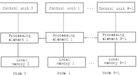
The classical von Neumann machine is an example of SISD machines. In Flynn’s taxonomy, the most general architecture is the MIMD system. In this system a collection of autonomous processors operate on their own data streams. MIMD systems, unlike SIMD systems, are asynchronous. The synchronization among processors, also called processing units, is achieved through appropriate message passing at specified time intervals. Whereas, in SIMD systems there is a global CPU devoted exclusively to control, and a large collection of subordinate ALUs each with its own memory [4]. A schematic of a MIMD computer is shown below [1]:
Figure 1. Schematic of a MIMD system
The MIMD system depicted in Figure 1. is a sample of Distributed-Memory MIMD systems. In this MIMD system, each processor has its own memory. A processor/memory pair is called a node, and nodes are connected via a network. MIMD systems, where each CPU has access to different memory modules are called Shared-Memory MIMD systems [4].
2.2. Beowulf Clusters
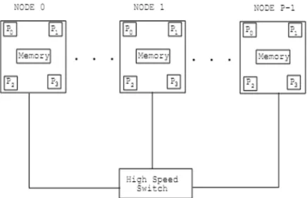
The most popular and cost-effective approach to parallel computing is cluster computing. A cluster is constructed of commodity components and runs com-modity software, such as Linux operating system. The prototype of PC-Clusters, also called Beowulf Clusters, is the Generic Parallel Computer which is depicted in the Figure 2. The clusters are dominating high performance computing both on the scientific as well as the commercial front [1].
Figure 2. Schematic of Generic Parallel Computer
The first PC cluster was designed in 1994 at NASA Goddard Space Flight Center to achieve one Gigaflop. Specifically, 16 PCs were connected together using a standard Ethernet network. Each PC had an Intel 486 microprocessor with sustained performance of about 70 Megaflops. This first PC cluster was built for only $40,000 compared to $1 million, which was the cost for a commercial equivalent supercomputer (the fastest computer of its time) at that time. It was named Beowulf after the lean hero of medieval times who defeated the giant Grendel [1]. After this project, this kind of clusters has been called as Beowulf Clusters.
As another example of using Beowulf cluster for throughput is Google, which uses over 15000 commodity PCs with fault tolerant software to provide a high-performance Web search service [5].
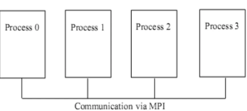
2.3. The Message-Passing Programming Paradigm
In parallel computing the divide-and-conquer approach is used as a strategy for solving problems. The problem is divided into manageable pieces which are further processed concurrently by individual computing nodes. The process of dividing a computation into smaller parts is called decomposition. This ap-proach is just another view of the message passing paradigm, one of the most widely used approaches for programming parallel computers. In programs im-plemented with this model, concurrent processes communicate with each other by means of messages.
The message-passing interface, abbreviated as MPI, represents a standard ap-plication programming interface (API), which is used for developing parallel programs in C/C++ or Fortran. MPI provides an infrastructure for the com-munication among the nodes. MPI is depicted in the Figure 3 [1].
Figure 3. Schematic of MPI processes working together
The MPI library contains many routines, however the six routines which form the minimal set of MPI routines are listed in the Table 2 [6].
Table 2. The minimal set of MPI routines
Most MPI programs are written using the single program multiple data (SPMD) approach. In this approach, different processes can execute different statements by branching within the program based on their ranks. There is a master process which receives the results (via the MPI_Recv routine) of other processes, where these processes send results via the MPI_Send routine. All of the nodes exe-cute the same program, however somewhere in the program there is a control statement like if (my_rank == 0) { // collect results } else {
// send result to master }
where the program behaves differently in the master node and differently in other nodes (in the piece of code above the master node is assumed to have the rank 0) [4, 6].
3. Installation of the Environment 3.1. Computing Nodes
For the environment eight computers with Celeron° CPU’s has been providedR by the school administration. Basic architecture of each computer is the same: CPU is 1.4 GHz and the capacity of memory is 512 MB.
3.2. Operating System
In general, Linux operating system is used for Beowulf Clusters. For our envi-ronment Fedora 11 distribution was used. The main factor for choosing Fedora was that it is a continuation of Red Hat Linux for community. Many other Beowulf Clusters built earlier were based on Red Hat [10]. Another reason was that Fedora is always free for anyone to use, modify, and distribute [11]. An-other motivational factor was that it is being used by Linus Torvalds, author of the Linux kernel [12]. At the time of installation, Fedora 11 was the latest version of the operating system. These were sufficient reasons for us, having no experience in Linux, to choose a Linux distribution for the environment. Each computer was assigned a unique name in the format C#, where C is used as prefix standing for Cluster and # was replaced with a digit starting from 0. On each computer a user with the username cluster and with the same password was created.
3.3. Local Area Network
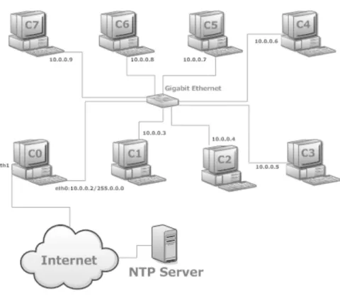
Eight computers have been connected using a Gigabit switch. A network has been configured with the 10.0.0.1/255.0.0.0 IP address configuration [7]. Only computer named C0, which is used as the master computer in the parallel ar-chitecture, has one more network adapter, and has been used for connecting to the Internet in order to synchronize its clock with a Network Time Protocol server. Then, other seven slave computers have been configured such that C0 is the NTP Server for them. Figure 4 shows a diagram of configuration. 3. 4. MPICH2 Installation
MPICH2 is a high-performance and widely portable implementation of the Mes-sage Passing Interface (MPI) standard (both MPI-1 and MPI-2) [13]. MPICH2 is installed only on the master computer C0. Then using the Network File Sys-tem (NFS) of Linux OS, the folders containing binaries required for running programs in parallel are shared to other computers. Using the mount command these slave computers are mounted to these folders.
Figure 4. Diagram of the Cluster 4. Sample Program: Parallel Numerical Integration
In this program the definite integral of a function is calculated using the trape-zoidal rule. However, the trapetrape-zoidal rule is implemented using the parallel computing methods, i.e., the usual serial algorithm is parallelized.
4.1. Trapezoidal Rule
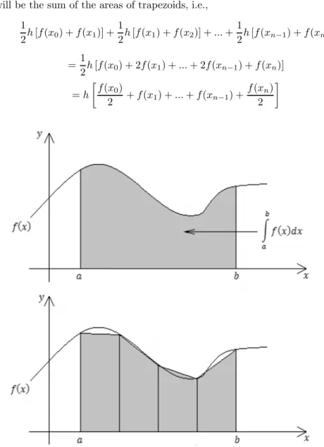
In this rule, the region, which is the area aimed to be calculated, is partitioned into trapezoids. Each trapezoid has its base on the horizontal axis, vertical side, and its top joining two points on the graph of ().
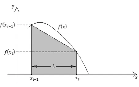
Assuming that all the bases have the same length, if there are n trapezoids then the base of each will be =− . The area of the i th trapezoid is
1
2 [ (−1) + ()] So the approximate area of the definite integral
Z
will be the sum of the areas of trapezoids, i.e., 1 2 [ (0) + (1)] + 1 2 [ (1) + (2)] + + 1 2 [ (−1) + ()] = 1 2 [ (0) + 2 (1) + + 2 (−1) + ()] = ∙ (0) 2 + (1) + + (−1) + () 2 ¸
Figure 6. The th trapezoid
It is now easy to program a computer to solve this problem. In order to par-allelize this problem it is necessary to partition the interval according to the number of processors [4].
4.2. A Few Words about Mathematical Parallelism
Consider the problem of finding the maximum in each pair of a set of N num-bers, i.e., max( ) = 1 2 If we solve this problem in N nodes, then N instances can be solved simultaneously. This is an example of perfect mathe-matical parallelism. These problems are referred to as Embarrassingly Parallel problems. In the case of determining the absolute maximum number in the pairs, interdependencies among data is introduced and the perfectness is broken [1].
Another problem is finding the sum of the first N numbers, i.e.,
X =1
It takes N-1 number of additions to solve this problem in one processor. If it takes the computer a time to perform an addition, then the total time required is 1= ( − 1). If we partition the domain 1,2,. . . , into parts (it is assumed that is evenly divisible by ), where is the number of processors, or nodes, then we can compute each sub-sum simultaneously using one processor for one sub-sum, and then by summing sub-sums we find the final result. If =0, 1,..., −1denotes each processor’s rank in our parallel computer, then the sub-sum performed by each processor is
(+1) X = +1
The time required for solving this problem in processors is = ( −1)+ ( − 1) + , where C represents the time to collect the results from sub-sums. The speed-up of this method is
= 1 =¡ ( − 1) − 1 ¢ + ( − 1) + = − 1 ¡ + − 2 ¢ +
Here represents the communication-to-computation time. If this relative value is very small it can be neglected and for very large the speed-up ap-proaches P, i.e., ≈ which is the theoretical maximum speed-up.
Another model for speed-up factor, proposed by Gene Amdahl in 1967, which is referred to as Amdahl’s Law, assumes that some percentage ()of the pro-gram cannot be parallelized, and that the remaining ((1−) is perfectly parallel. Neglecting any communication delays, this model is formulized as
= 1 ³ +1− ´1 = ³ 1 +1− ´
If → ∞ then → 1. This is an important result which implies that after some point increasing the number of processors does not speed-up the computation. For example, for = %2 = 002 and P=200 we have200= 4016, i.e., our efficiency is %20.08 [1].
4.3. Program Implementation
As in the summing problem above, this problem can be parallelized by partition-ing the interval [a, b] accordpartition-ing to the number of processors, and then assignpartition-ing to each processor a sub-interval for calculating the integral for this sub-interval. The mathematical foundation of the approach is the rule of the definite integral that states if () is continuous on [ ] and for a number , then
Z () = Z () + Z ()
Table 3
It is easy to see that in order to calculate integral each process needs • Its rank, i, (obtained by calling MPI_Comm_rank),
• Total number of processes, P, executing the program (obtained by calling MPI_Comm_size),
• The values a,b,n which are supplied by the user of the program.
The program is written in the C++ language. Variables whose contents are significant in individual processes are preceded with the local_ suffix, for doc-umenting purposes. Program consists of four functions:
• int main(int argc, char ** argv), entry point of the program. Every MPI program must begin with the MPI_Init and end with the MPI_Finalize functions.
• void get_data(float* a_ptr, float* b_ptr, int* n_ptr, int my_rank, int p), this function asks user for the values,b,n, to enter only if it runs in the master process, i.e., process with the rank 0. If so, sends these values to other processes via the MPI_Send function. Otherwise, receives sent values from the master process.
• float calculate_integral(float local_a, float local_b, float local_n,float h), this function does the calculation of integral according to the trapezoidal rule mentioned above.
• float f(float x), this is the() function. It can be any function computable in computer, for this program it is the square function () = 2.
In different places of the program there is control if (my_rank == 0), which reflects the approach used in this program, i.e., the SPMD approach.
The program is listed bellow [4]. #include iostream #include "mpi.h" using namespace std; float f(float x) {
return x*x; }
float calculate_integral(float local_a, float local_b, float local_n,float h) {
float integral; // store result in integral float x;
int i;
integral = (f(local_a) + f(local_b))/2.0; x = local_a;
for (i = 1; i = local_n-1; i++) { x = x + h; integral = integral + f(x); } integral = integral * h; return integral; }
void get_data(float* a_ptr, float* b_ptr, int* n_ptr, int my_rank, int p) { int source = 0; int dest; int tag; MPI_Status status; if (my_rank == 0) {
cout "Enter a:"; cin *a_ptr; cout "Enter b:"; cin *b_ptr; cout "Enter n:"; cin *n_ptr;
for (dest = 1; dest p; dest++) {
tag = 0;
MPI_Send(a_ptr, 1, MPI_FLOAT, dest, tag, MPI_COMM_WORLD); tag = 1;
MPI_Send(b_ptr, 1, MPI_FLOAT, dest, tag, MPI_COMM_WORLD); tag = 2;
MPI_Send(n_ptr, 1, MPI_INT, dest, tag, MPI_COMM_WORLD); }
} else { tag = 0;
MPI_Recv(a_ptr, 1, MPI_FLOAT, source, tag, MPI_COMM_WORLD, &status);
tag = 1;
MPI_Recv(b_ptr, 1, MPI_FLOAT, source, tag, MPI_COMM_WORLD, &status);
tag = 2;
MPI_Recv(n_ptr, 1, MPI_INT, source, tag, MPI_COMM_WORLD, &sta-tus);
} }
int main(int argc, char ** argv) {
int my_rank; // my process rank int p; // number of processes float a = 0.0; // left endpoint float b = 2.0; // right endpoint int n = 1024; // number of trapezoids float h; // trapezoid base length
float local_a; // left endpoint my process float local_b; // right endpoint my process
int local_n; // number of trapezoids for my calculation float integral; // integral over my interval
float total; // total integral
int source; // process sending integral int dest = 0; // all messages go to 0 int tag = 0;
MPI_Status status;
// let the system do what it needs to start up MPI MPI_Init(&argc,&argv);
// get my process rank
MPI_Comm_rank(MPI_COMM_WORLD, &my_rank); // find out how many processes are being used
MPI_Comm_size(MPI_COMM_WORLD, &p); get_data(&a,&b,&n, my_rank, p);
h = (b - a) / n; // h is the same for all processes local_n = n / p; // so is the number of trapezoids
// length of each process’s interval of integration = local_n*h // so my interval starts at:
local_a = a + my_rank * local_n * h; local_b = local_a + local_n * h;
integral = calculate_integral(local_a, local_b, local_n, h); // add up the integral calculated by each process
if (my_rank == 0) {
total = integral;
for (source = 1; source p; source++) {
MPI_Recv(&integral, 1, MPI_FLOAT, source, tag, MPI_COMM_WORLD, &status);
total = total + integral; }
} else {
MPI_Send(&integral, 1, MPI_FLOAT, dest, tag, MPI_COMM_WORLD); }
// print the result if (my_rank == 0) {
cout "With n=" n " trapezoids, our estimate" endl; cout "of the integral from " a " to " b " = " total endl;
}
// shut down MPI MPI_Finalize(); return 0;
}
To compile and execute the program we write the following commands from the shell of the C0 machine:
[cluster@C0 ∼]$ mpicxx -o /tmp/cluster/mpich2-1.2.1p1/examples /parallel_integral /tmp/cluster/mpich2-1.2.1p1/examples /parallel_integral.cpp [cluster@C0 ∼]$ mpdboot -n 8 [cluster@C0 ∼]$ mpdtrace -l C0_34343 (10.0.0.2) C7_49570 (10.0.0.9) C1_53946 (10.0.0.3) C2_48341 (10.0.0.4) C4_35981 (10.0.0.6) C6_37279 (10.0.0.8) C5_51315 (10.0.0.7) C3_46985 (10.0.0.5)
[cluster@C0 ∼]$ mpiexec -l -n 8 /tmp/cluster/mpich2-1.2.1p1/examples /parallel_integral
Enter a:2 Enter b:3 Enter n:1024
With n=1024 trapezoids, our estimate of the integral from 2 to 3 = 6.33333
Commands provided by MPICH2 are mpicxx (used to compile the MPI pro-grams written in C++), mpdboot (starts a set of multiprocessing daemons on a list of machines), mpdtrace (lists all MPD daemons that are running), and mpiexec(runs MPI program on machines running MPD daemons) [13] 5. Conclusion
This environment has given us a great experience in installing Beowulf Clusters. During the installation, problems concerning MPICH2 were hard to solve. En-vironment has been used for solving only simple problems. In the future work this environment will be tested with more serious problems.
We are going to study methods of solving differential equations using parallel computing methods and implement these solutions on this environment. References
1. Karniadakis E. M., Kirby R. M., 2003, Parallel Scientific Computing in C++ and MPI: A Seamless Approach to Parallel Algorithms and their Implementation, Cambridge University Press
2. Parhami B., 2002, Introduction to Parallel Processing, Kluwe Academic Publishers 3. Heath M.T., 1997, Scientific Computing: An Introductory Survey, The McGraw-Hill Company
4. Pacheco P. S., 1997, Parallel Programming with MPI, Morgan Kaufmann Publish-ers, Inc.
5. Gropp W., Lusk E., Sterling T., 2003, Beowulf Cluster Computing with Linux, Second Edition, The MIT Press
6. Grama A., Gupta A., Karypis G., Kumar V., 2003, Introduction to Parallel Com-puting, Second Edition, Addison Wesley
7. Negus C., Foster-Johnson E., 2009, Fedora° 10 and Red HatR ° Enterprise LinuxR °R Bible, Wiley Publishing Inc.
8. http://searchcio-midmarket.techtarget.com/sDefinition/0„sid183_gci213140,00.html, 07.07.2010 9. https://computing.llnl.gov/tutorials/parallel_comp/,08.07.2010 10. http://www.beowulf.org/overview/projects.html,16.06.2010 11. http://fedoraproject.org/, 17.06.2010 12. http://www.simple-talk.com/opinion/geek-of-the-week/linus-torvalds,-geek-of-the-week/, 17.06.2010 13. http://www.mcs.anl.gov/research/projects/mpich2/, 17.06.2010