Reducing Processing Time for Histogram PMHT Algorithm
in Video Object Tracking
Ahmet Güngör Pakfiliz
Department of Electrical and Electronics Engineering, Başkent University School of Engineering, Ankara, Turkey
Corresponding Author: Ahmet Güngör Pakfiliz E-mail: [email protected] Received: 27.08.2017 Accepted: 10.05.2018 © Copyright 2018 by Electrica Available online at http://electrica.istanbul.edu.tr DOI: 10.26650/electrica.2018.36247
Cite this article as: Pakfiliz AG. “Reducing Processing Time for Histogram PMHT Algorithm in Video Object Tracking”, Electrica, vol. 18, no: 2, pp.
121-132, 2018.
ABSTRACT
This paper describes a novel approach for reducing the processing time of the histogram probabilistic multi-hypothesis tracker (H-PMHT) algorithm in video applications. Video data of flying vehicles is taken from surface to air, and a temporal difference-based technique is applied to video frames for meeting the intensity demands of H-PMHT algorithm. This technique also enables discrimination between objects and eliminates clutter. Variations between the structures of the standard and the improved version of H-PMHT algorithms are described. In addition, the improved H-PMPT is compared with the standard H-PMHT and another approved tracking algorithm to evaluate the performance and processing time reduction ratings.
Keywords: Improved H-PMHT, Pixel Wise Difference, Surface to air, Video Tracking
Introduction
TRACKING requires high precision and real-time applications. For sensors taking continuous and bulky data streams such as video data, real-time operation is difficult to achieve using whole sensor data. When conventional tracking algorithms are used for video object tracking real-time may be achieved, but only at the expense of some level of precision due to transfor-mation of the data into a suitable measurement domain [1-3]. These transfortransfor-mations also take the physical shapes of the targets, which are projected onto the image frame, up to a level and convert them to point measurement, thus adding to measurement error. Coping with a high amount of data streams is necessary in order to reach high precision rates in video object tracking. Therefore, target shape and intensity-based algorithms get the edge on point-mea-surement trackers [4, 5]. Reliable and uninterrupted track information is essential for most of the applications, especially in a background of a high clutter environment and a lack of sen-sor capacity. In order to detect the target location from the data stream, high intensity pixel clusters should be searched from data streams, and it should be decided whether or not they emerge from target or clutter. H-PMHT is a feasible method for handling data streams, and for tracking objects reliably and uninterruptedly.
The H-PMHT is basically an Expectation Maximization (EM) based algorithm which was devel-oped for target tracking in dense clutter environment by processing a considerable amount of data streams [6]. H-PMHT is a track-before-detect (TkBD) algorithm and entire video data is used as the measurement. It processes detection and tracking operations simultaneously. H-PMHT maintains tracking performance for low SNR values, where the target is not easily distinguished from the noise-cluttered background of any given frame. The original H-PMHT assumes that the signature of each target in the sensor frame area is known. In this particular case, the signatures are in the Gaussian distribution, and the means of these Gaussians are linearly related to the states of the targets. In imagery applications, the target signature is the physical shape of the target projected onto the image frame. This shape can be time-varying and complicated [7]. H-PMHT provides considerably satisfactory results for one dimensional and two dimensional applications [8-10]. In these applications spreading of the target
inten-sities presents almost a linear-Gaussian distribution. Moreover, for non-linear and non-Gaussian applications a particular solu-tion is presented in with particle filters. In addisolu-tion, a video tracking application is presented in with a specially processed video data, and a modified H-PMHT, which is called H-PMHT with Random Matrices (H-PMHT-RM) [11, 12].
The main purpose of this study is to reduce the processing time of the H-PMHT algorithm without deterioration in per-formance. For this purpose, we needed to obtain available and reliable measurement data in order to discriminate moving objects and represent them with a higher intensity area than the stationary background. Firstly, video data belonging to air vehicles is taken in true color (RGB) from surface to ground. Then a temporal difference processing technique is applied to filter moving objects from the stationary background. Thereby, proper data streams composed of moving objects and back-ground are obtained for processing with H-PMHT.
Two important obstacles need to be overcome to reduce the processing time of H-PMHT. One of them is the dynamic struc-ture of the video data, because in video tracking applications tracker processes data sequentially, not in a batch structure. The other is the long processing time, which is due to the structure of H-PMHT. By setting the batch number to one and replacing the smoother filter by a Kalman filter it becomes pos-sible to overcome the issue of data processing sequence. On the other hand, dealing with the long processing time is a chal-lenge. The aim of this study is not to completely eliminate this issue, but to reduce the processing time by improving H-PMHT algorithm. For this purpose, not only algorithm improvement, but also an amendment needs to take place in the basic struc-ture of the H-PMHT in order to reduce the processing time while continuing tracking and keeping estimation error within a reasonable limit. The resulting algorithm is called Improved H-PMHT (I/H-PMHT).
The tracking performance of I/H-PMHT for video data is given in the experimental study section. In this section, the obtained results are also compared in terms of processing time and esti-mation error with standard H-PMHT, and Interacting Multi Model Probabilistic Data Association with Amplitude Information (IM-MPDA-AI) algorithms for different conditions and cases [13].
Measurement Model
This study intends to reduce the processing time of H-PMHT al-gorithm. To that end, RGB video is taken for various aircrafts and each frame is processed separately according to time sequence. First of all, RGB images are converted into intensity images. Na-tional Television System Committee (NTSC) standard for trans-forming RGB to grayscale, defined in, is given as follows,
I x, y
( )
=0.2989R x, y( )
+0.587G x, y( )
+0.114B x, y( )
(1) After that, pixel-wise difference function is obtained using a similar process as that described in [14, 15]. The aim of this process is to obtain frame data for frames k and k+Δ, then sub-tract them and take the absolute value of the difference. This
is followed by the thresholding process, and the remaining values give information about the movement. k represents the instantaneous frame time, and Δ represents the sampling peri-od of frames. As long as the object does not move too fast, the detected regions of the object are reduced. However, this pro-cess leaves a ghost where the object was located, and a large part of the object cannot be detected unless the object moves fast [16]. Additional processing is required to reduce the ghost effect by adapting the measurement data to the situation. For this purpose, we obtained the difference from the former to the following time sequence as follows.
I
dif(x, y) = I
k(x, y) − I
k+Δ(x, y)
(2)There are two additional steps that must be performed to ob-tain the measurement model. The first step is thresholding the unwanted ghosts due to the former time k. As a result of the operation in equation (2), negative and positive intensity dif-ferences are obtained. Indeed, high magnitude negative values are out of the scope of this work, because they are the reflec-tions of former target echo. In order to get rid of these spurious intensities, negative values are converged to noise floor, and positive values are taken directly. Thus the intensity level of each cell M(x,y) is given as follows,
(3)
M x, y
( )
=
I
Noise_ floor+
rand
, I
dif( )
x, y
≤
0
I
dif( )
x, y
=
I
dif( )
x, y
, I
dif( )
x, y
>
0
⎧
⎨
⎪
⎩⎪
where INoise_floor represents the intensity of the noise floor, which is defined as the intensity level of pixels that do not originate from the target or the clutter. Idif(x,y) represents the intensity of
differences, and rand is the uniformly distributed pseudoran-dom number.
The second step taken in order to obtain the measurement mod-el is intensity pruning. The square root of M(x,y) values of intensi-ties are taken as in equation (4). Thus, an excessive increment in dynamic range and high intensity clutters are prevented.
(4)
I
PDIM
( )
x, y
=
M x, y
( )
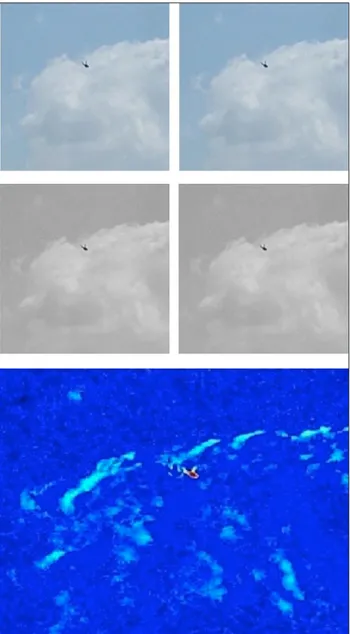
The measurement model is achieved after obtaining pixel intensity levels for each pixel of the sensor area. Because the data is obtained using the difference of pixel intensities of the sequential video frames, it is defined as Pixel-wise Difference Intensity Modulated (PDIM) data. RGB images of sequential video frames of an aircraft, intensity images related to them, and resulting PDIM data image are given in Figure 1. The scan steps between them are 3 frames, in other words Δ=3.
Using PDIM method, stationary parts of the image can be elim-inated or reduced to acceptable levels, since intensity levels of
pixels related to stationary parts will remain the same at con-secutive times and the difference of the intensity levels will be zero, small motions on some parts of stationary objects or a slight vibration of camera will result in a non-zero difference level, and it is taken into calculations as background clutter. In this study PDIM data is used for surface to air video object tracking with improved H-PMHT algorithm.
Basic Structure of H-PMHT
The H-PMHT algorithm is introduced in [6, 8, 9] with its theory and derivations. Before entering the details of H-PMHT algo-rithm, its parametric TkBD structure is discussed. In tradition-al tracking methods, thresholding, clustering, extracting and
tracking procedures are carried out consecutively. On the oth-er hand, TkBD method poth-erforms all the steps concurrently [17, 18]. TkBD merges detection and estimation phases by eliminat-ing the detection algorithm from the process and supplyeliminat-ing the whole sensor frame directly to the tracker. This increases trace accuracy and allows the tracker to keep track for low SNR targets [19]. The H-PMHT algorithm inherently includes the TkBD capability and makes it possible to obtain extended ob-ject traces directly from an image sequence.
Only a general structural outline for H-PMHT is given here. H-PMHT is mainly developed from PMHT, and all derivations of PMHT arise from Expectation Maximization (EM) method [20]. The purpose of using the EM process in the H-PMHT algorithm is to assign histogram distribution to the model components and to designate the precise position of the shots as missing data. It also allows for unobserved cells with abstract sensor pixels that do not convey any data. The probability of the miss-ing data is determined in the E-step and the state estimates are refined in the M-step. Initialization and iteration steps of H-PM-HT according to E and M-steps are given below.
Initialization of H-PMHT Algorithm
Initialization steps must be defined before iterations are de-scribed. At the beginning of each iteration mixing proportions (
ˆ
πtk( )0 are determined for background and all target models (k=0, 1,…, M), and for batch sequence t = 1 = 1,K,T, for which T≥1
denotes the number of scans in a batch of measurement, as follows,
(5)
ˆπ
tk( )
0>
0 and ˆπ
t0( )
0+ ˆ
π
t1( )
0+!+ ˆ
π
tM( )
0=
1
In addition, for
k =1,…, M
, for which M≥1 denotes the number of targets, the following is initialized,- Target State Sequence:
ˆx
0k 0( )
, ˆx
1k 0( )
,…, ˆx
Tk 0( )
- Measurement Covariance Sequence:
ˆR
1k( )
0,…, ˆR
Tk( )
0 - Target Covariance:ˆQ
k
0
( )
The H-PMHT algorithm consists of repeated iteration steps for each batch sequence
t =1,…,T
. Some of these iteration steps stem from Expectation and Maximization, the remainder comes from Kalman smoothing filter. Throughout the iterations the dynamic matrix F and measurement matrix H are assumed as constant or time invariant. Iteration steps with respect to Ex-pectation, Maximization, and Kalman smoothing processes are given in the following subsections.Expectation
Step 1. Total Sensor Probabilities (TSPs)
First, Target Cell Probabilities (TCP) are calculated for batch length t=1,...,T for all cells ℓ=1,…,S and for all target models, including background k=0,1,…,M . S represents the number of
Figure 1. Proposal structure video images for an aircraft at k and
k+3 frames (above); Intensity images of them [middle, and PDIM (bottom)] data obtained using them
whole cells in the sensor area. For the background and targets TCPs are calculated as follows,
(6)
P
tkℓ i+1 ( )=
1
S
if k = 0
N τ ;H
tkˆx
tk i ( ), ˆR
tk i ( )(
)
dτ if k =1,…, M
Bℓ( )t∫
⎧
⎨
⎪⎪
⎩
⎪
⎪
where τ represents the variable term of N(∙) Gaussian PDF. Total cell probabilities are obtained by summing the product of TCPs and mixing proportions for all target models and back-ground as in equation (7).
P
(7) tℓ i+1( )
=
ˆπ
tk i( )
P
tkℓ i+1( )
k=0 M∑
Finally, TSPs are attained using only displayed cells or cells with measurement ℓ=1,…,L(t) as follows;
P
(8) t i+1( )
=
P
tℓ i+1( )
ℓ=1 L t( )
∑
Step 2. Expected Measurements (EMs)EMs are calculated as in equation (9) for t=1,...,T, and ℓ=1,…,S.
(9)
z
tℓ i+1 ( )=
z
tℓ1≤ ℓ ≤ L t
( )
Z
tP
tℓ i+1 ( )P
t( )i+1⎛
⎝
⎜
⎜
⎞
⎠
⎟
⎟
L t
( )
+1≤ ℓ ≤ S
⎧
⎨
⎪⎪
⎩
⎪
⎪
where Zt represents L1 norm of displayed cells
B1
( )
t ,…, BL(t)( )
t{
}
and it is defined as follows,Z
t=
z
tℓℓ=1
L t
( )
∑
(10)Maximization
Step 3. Cell-level Centroids (CCs):
CCs are calculated by using equation (11).
(11)
!
z
tkℓ( )
i+1=
1
P
tkℓ( )
i+1τ N τ ; H
tkˆx
tk i( )
, ˆR
tk i( )
(
)
Bℓ( )
t∫
dτ
Using CCs, synthetic measurements are obtained as follows;!
z
tk( )
i+1=
z
tℓ i+1( )
℘
tkℓ( )
⎡
⎣
⎤
⎦!z
tkℓ i+1( )
ℓ=1 S∑
z
tℓ( )
i+1℘
tkℓ( )
⎡
⎣
⎤
⎦
ℓ=1 S∑
→ ℘
tkℓ=
P
tkℓ( )
i+1P
tℓ( )
i+1⎧
⎨
⎪
⎩⎪
⎫
⎬
⎪
⎭⎪
(12)Step 4. Synthetic Covariance Matrices
Synthetic measurement matrices given in equation (13) are ob-tained for t = 1,...,T, and k = 1,...,M.
(13)
R
!
tk i+1( )
=
ˆR
tk i( )
ˆπ
tk( )
iz
tℓ i+1( )
℘
tkℓ( )
⎡
⎣
⎤
⎦
ℓ=1 S∑
Also, for t = 0,1,...,T–1 synthetic measurement covariance
ma-trices are calculated as follows:
(14)
Q
!
tk i+1( )
=
P
t+1 i+1( )
Z
t+1ˆQ
k i( )
Step 5. Mixing Proportions
Mixing proportions are calculated for t = 1,...,T and k = 0,1,...,M:
(15)
ˆπ
tk i+1( )
=
ˆπ
tk i( )
z
tℓ i+1( )
℘
tkℓ( )
⎡
⎣
⎤
⎦
ℓ=1 S∑
ˆπ
t ʹ( )
kiz
tℓ( )
i+1( )
℘
tkℓ⎡
⎣
⎤
⎦
ℓ=1 S∑
ʹ k =0 M∑
Kalman Smoothing Filter
To obtain estimated target states a Kalman smoother filter is applied. This portion of the algorithm is composed of forward and backward filters.
Step 6. Forward Filter
The forward Kalman smoother filter for t=0, 1,…, T-1 is applied using synthetic measurements in order to refine target state es-timates. At this point dummy expectation is taken as !y00
i+1
( )( )k =0
and dummy covariance is P
00
i+1
( )
( )
k =0. The equations of forward filter are given in (16)-(18)P
t+1t( )
i+1k
( )
=
FP
t t( )
i+1( )
k
F
∗+ !
Q
tk i+1( )
(16)W
t+1( )i+1k
( )
=
P
t+1t( )i+1( )
k
H H P
t+1t( )i+1( )
k
H
∗+
R
t+1,k i+1 ( )(
)
−1 (17)P
t+1t+1( )
i+1( )
k
=
P
t+1t( )
i+1( )
k
−
W
t+1( )
i+1( )
k
H P
t+1t( )
i+1( )
k
(18)
!
y
t+1t+1( )i+1k
( )
=
F!y
t t( )i+1( )
k
+
W
t+1( )i+1( )
k
!
z
t+1,k i+1 ( )−
H!y
t t i+1 ( )( )
k
(
)
(19)where Wt+1(i+1) is filter gain, and F is state transition matrix,
Step 7. Backward Filter
The equation of backward filter for t = T – 1,....1 is given as
follows: (20)
ˆx
tk( )
i+1= !
y
t t( )
i+1( )
k
+
P
t t( )
i+1( )
k
F
∗P
t+1t i+1( )
( )
k
(
)
−1In
( )
where In
= ˆ
x
t+1,k( )
i+1−
F!y
t t( )
i+1( )
k
Step 8. Estimated Covariance Matrices
First cell-level measurement covariance is calculated,
(21)
ˆR
tkℓ( )
i+1=
N τ ;H
tkˆx
tk i( )
, ˆR
tk i( )
(
)
E E
∗dτ
Bℓ( )
t∫
P
tkℓ( )
i+1where E = τ − H
tkˆx
tk( )
i+1The estimated measurement covariance matrix is calculated as given in equation (22): (22)
ˆR
tk i+1( )
=
z
tℓ i+1( )
℘
tkℓ( )
⎡
⎣
⎤
⎦
ℓ=1 S∑
ˆR
tkℓ i+1( )
z
tℓ( )
i+1( )
℘
tkℓ⎡
⎣
⎤
⎦
ℓ=1 S∑
And the last operation shown in equation (23) of the iteration is to obtain estimated target covariance matrices for all the target models except for the background.
(23)
ˆQ
k i+1 ( )=
Z
tP
t( )i+1⎛
⎝
⎜
⎜
⎞
⎠
⎟
⎟ ˆx
tk i+1 ( )−
Fˆx
t−1,k i+1 ( )(
)
ˆx
tk( )i+1−
Fˆx
t−1,k( )i+1(
)
∗ t=1 T∑
Z
tP
t i+1 ( )⎛
⎝
⎜
⎜
⎞
⎠
⎟
⎟
t=1 T∑
Variations of the Algorithm
Histogram probabilistic multi-hypothesis tracker is a strong and reliable tracking algorithm and originally developed for data streams. However, it is not conformed to real time appli-cations. The aim of this study is to converge real time tracking or reduce the processing time of H-PMHT algorithm without terminating tracking for video applications. First of all, video data is converted to PDIM data in order to clutter effects and enhance target detectability. Then some improvements are ap-plied to mathematical operations, in particular by taking the practical advantage of two-dimension, and also some amend-ments are applied to the algorithm itself. This work was done by adding intensity information that can be thought of as a third dimension in two-dimensional space. For this reason, this study is regarded as a two-dimensional application and the assumptions in [10] can be implemented. The most important aspect of these assumptions is that x and y axes are
statisti-cally independent of each other. Another assumption for the process is that there is no pre-information about point spread function of the objects. They mostly retain their original shape and this shape is not similar to linear-Gaussian distribution. It will be proper to state that there is no revision on the se-quence of EM based iteration steps. The main difference takes place in the batch structure of EM iteration. In this study batch structure is eliminated and its structure is converted to single scan algorithm. To overcome a priori information absence, a priori density obtained via earlier measured data is used as stated in [6]. Using single scan structure is more viable than batch structure for converging real-time video object tracking applications. By using single scan structure, smoothing filter turns to Kalman Filter (KF), but in this case not much processing time reduction takes place. This is the first step for the reduc-tion of processing time. The improvements and amendments are described separately in the following subsections.
Operational Improvements
In this section, no algorithmic amendments, but operation im-provements of the algorithm are described. To achieve this aim the batch structure is turned into single scan algorithm, but multi iteration structure is preserved. The inspected part in this section is the most time-consuming fragment of the H-PMHT process which is spent in calculation of integration operations. These operations are
- Target Cell Probabilities Ptkℓ( )i+1
, - Cell Level Centroids
z
tkℓ( )
i+1 ,- Cell Level Meas. Covariance Contributions
ˆR
tkℓ( )
i+1.In two-dimensional case these three expressions are normally calculated for x and y axes separately, then corresponding values of each pixel are multiplied with each other to obtain the overall value. The total number of integration (NoI) is calculated by sum-ming up NoI of the above three expressions. In this context NoI of a sensor area with “200 x 200 pixels” is calculated as follows.
For x-axis:
NoI P
tkℓ x i+1( )
{ }
=
NoI !z
tkℓ x i+1( )
{ }
=
NoI ˆR
tkℓ x i+1( )
{ }
=
40000
For y-axis:NoI P
tkℓ y i+1( )
{ }
=
NoI !z
tkℓ y i+1( )
{ }
=
NoI ˆR
tkℓ y i+1( )
{ }
=
40000
For two dimensions:
NoI P
{ }
tkℓ( )
i+1=
NoI !z
{ }
tkℓ( )
i+1=
NoI ˆR
{ }
tkℓ( )
i+1=
2× 40000
= 80000
Total NoI:
This phase increases the process time exponentially for linear increasing of sensor dimensions. To decrease the processing time, an improvement method is applied to H-PMHT operation in order to obtain Target Cell Probabilities, Cell Level Centroids, and Cell Level Measurement Covariance Contributions. For this purpose, only the elements of the first row of x axis contribu-tion and only the elements of the first column of y axis contri-bution are calculated. Thus, NoI for sensor area with “200 x 200” pixels can be shown as follows.
For x-axis:
NoI P
tkℓ( )i+1x{ }
=
NoI !z
{ }
tkℓ( )i+1x=
NoI ˆR
{ }
tkℓ( )i+1x=
No.of Row
NoR
(
)
For y-axis: NoI Ptkℓy i+1 ( ){ }
=NoI !ztkℓy i+1 ( ){ }
=NoI ˆRtkℓy i+1 ( ){ }
= No.of Column NoC(
)
For two dimensions:
NoI P
tkℓ( )i+1{ }
=
NoI !z
{ }
tkℓ( )i+1=
NoI ˆR
{ }
tkℓ( )i+1=
NoR+ NoC
= 2× 200 = 400
Total NoI:
Total − NoI = 6× pixel − no.= 6× 400 = 2400
After finding the elements of the first row of x axis contribution for the three expressions, we then selected the other rows in the same way as the first row and established Target Cell Prob-abilities, Cell Level Centroids, and Cell Level Measurement Co-variance Contributions. Similarly, for y axis contribution, other columns are taken in the same way as the first column. In fact, the results obtained by taking integration for whole pixels of the sensor area using the classical method is the same as the reduced one. Thus, the NoI reduces from 480000 to 2400. A remarkable reduction in processing time is obtained and no reduction in accuracy occurs Applying this improvement ap-proximately 34 - 63% (differs for different sensor area) process time reducing with respect to standard H-PMHT is obtained. The results are given in the experimental study section.
Algorithm Amendments
In addition, some algorithm amendments were used in order to decrease processing time and adjust the algorithm structure to dynamic and real time conditions. These amendments are given in the following items.
Item 1. First of all, the batch structure of the H-PMHT algorithm
is converted to single scan algorithm, and the algorithm be-comes more suitable for dynamic applications, such as video object tracking [19]. A result of this conversion that backward filter is removed and the smoothing filter turns into KF. Because smoother filer turns to KF, the estimated target states
!
y
t|t(i+1)(k)
and dummy covariance matrix ( 1) |i
( )
t t
P
+k
are picked up from the previous frame step instead of initiate them for eachitera-tion. Also, the initiation process is eliminated and the output of the previous time will be the input of the next time.
Item 2. Reducing iteration number is another amendment for
reducing processing time. But reducing iteration number with-out taking necessary measures may be resulted with conver-gence insufficiency of state estimates to true position. In order to mitigate this risk, measurement covariance sequences in the initialization phase ˆRtk( )0 are selected compatible with the
tar-gets. Compatible means selecting initial measurement covari-ance low for small targets, and high for large targets.
Item 3. In order to reduce iteration number without increasing
the estimation error more than an allowable amount, an addi-tional measure is taken. In the fundamental theory of H-PMHT [6], some expressions are calculated for only displayed cells (B1(t),...,BL(t)(t)), without using the truncated ones (BL(t)+1(t),...,BS(t)).
These expressions are; L1 norm of measurements Zt , total
sensor probabilitiesPt( )i+1, and expected measurements z
tℓ i+1
( ) . The border level between displayed and truncated cells can be regarded as threshold level which comes from the struc-ture of H-PMHT. In fact, this is not exactly a threshold, because truncated cells are also counted in the calculations except the above expressions. Thus it may be called as Displayed Cell
Threshold-DCT. Selecting a higher DCT value will reduce the
number of steps required to converge the state estimates to the correct position. On the other hand, increasing the DCT ex-cessively may cause some target-based measurements to be incomplete.
Item 4. Using compatible initial measurement covariance ˆRtk( )0
and proper DCT, the iteration number may be reduced to one, and an additional reduction in processing time can be reached. Calculation of estimated measurement matrix ˆRtk( )i+1 is not
nec-essary for one iteration case.
-By using compatible initial measurement covariance ˆRtk( )0 and proper DCT, iteration number may be reduced to one, and an additional reduction in processing time can be reached. Calcu-lation of estimated measurement matrix ˆRtk( )i+1 is not necessary
for one iteration case.
After making these amendments approximately 8 -29% addi-tional process time reducing (differs for different sensor area) is obtained. This reduction takes place after operational im-provement, and the reduction rate is based on the CPU time of operational improvement applied H-PMHT, not the total CPU time rate. This case is different from operational improvements, because algorithm amendments result in sacrificing some ac-curacy, especially in low DCTs.
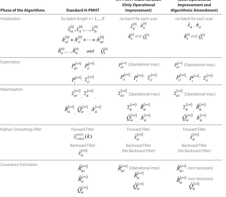
At the end of the improvement and amendment process the total decreasing process time converges to approximately 65%. The reduction amount decreases with big sensor area, and it increases with small sensor area. The detailed results are also given in the simulation section. The new version of the al-gorithm is named as improved H-PMHT (I/H-PMHT), and sche-matic structure is given in Table 1.
Experimental Study
The experimental trials were conducted for different scenari-os of single aircraft and chopper videscenari-os taken from surface to air. Video data was captured in true color (RGB) format with “640x480” pixels, using a 14.1 Mega-pixel camera. In the simu-lations the dimensions of sensor areas are selected “200x200”, “250x250”, and “300x300” pixels in order to evaluate CPU reduc-tion rate for different sensor areas.
The study is conducted in two-dimensional case, and the as-sumptions made in [10] are used. Additionally, pre-information about point spread function of the objects does not exist. They mostly retain their original shape and these shapes are quite different from the linear-Gaussian distribution.
To perform the operation, first the PDIM data is obtained us-ing the video data taken from surface to air in daylight. Then tracking process is applied to each PDIM data using I/H-PMHT algorithm. For benchmarking the obtained results in terms of process time reduction and performance each scenario is re-applied to standard H-PMHT and a trustworthy probabilistic algorithm IMMPDA-AI. This algorithm is a combination of IMM estimator and PDA technique [4, 5], and by adding amplitude information, the results obtained with IMMPDA-AI will be prop-er for a fair comparison with the results of I/H-PMHT. Thus, pro-cessing time shortening and tracking performances of I/H-PM-HT are compared with the counterparts of standard H-PMI/H-PM-HT and IMMPDA-AI.
Table 1. Structural Comparison between Standard H-PMHT and I/H-PMHT
Phase of the Algorithms Standard H-PMHT
I/H-PMHT Multi Iteration (Only Operational
Improvement)
I/H-PMHT One Iteration (Both Operational Improvement and Algorithmic Amendment)
Initialization for batch length t = 1,....T
ˆx
0k( )
0, ˆx
1k( )
0,…, ˆx
Tk( )
0ˆπ
t0( )
0+ ˆ
π
t1( )
0+!+ ˆ
π
tM( )
0ˆR
1k( )0,…, ˆR
Tk 0 ( )and
ˆQ
k 0 ( )no batch for each scan
ˆx
tk( )0 ,ˆπ
tk 0 ( ) ˆRtk 0 ( )and ˆQ k 0 ( )no batch for each scan
ˆx
tk,ˆπ
tk ˆRtk 0 ( )and ˆQ k 0 ( ) ExpectationP
tkℓ( )
i+1 ,P
tℓ i+1( )
P
t( )
i+1 ,z
tℓ i+1( )
P
tkℓ( )i+1 (Operational impr.)P
tℓ( )
i+1 ,P
t( )
i+1 ,z
tℓ( )
i+1P
tkℓ( )i+1 (Operational impr.)P
tℓ( )
i+1,P
t( )
i+1,z
tℓ i+1( )
Maximization!
z
tkℓ( )
i+1 ,z
tk i+1( )
,!
R
tk( )
i+1 ,Q
!
tk( )
i+1 ,ˆπ
tk( )
i+1!
z
tkℓ( )
i+1 (Operational impr.)z
tk( )
i+1 ,R
!
tk i+1( )
!
Q
tk( )
i+1 ,ˆπ
tk( )
i+1!
z
tkℓ( )
i+1 (Operational impr.)z
tk( )
i+1 ,R
!
tk i+1( )
!
Q
tk( )
i+1 ,ˆπ
tk( )
i+1Kalman Smoothing Filter Forward Filter
!
y
t+1|t+1(i+1)(k)
Backward Filterˆx
tk( )
i+1 Forward Filterˆx
tk( )
i+1 Backward Filter (No Backward Filter)Forward Filter
ˆx
tk( )
i+1Backward Filter (No Backward Filter) Covariance Estimation
ˆR
tkℓ( )
i+1ˆR
tk( )
i+1ˆQ
tk( )
i+1ˆR
tkℓ( )
i+1 (Operational impr.)ˆR
tk( )
i+1ˆQ
tk( )
i+1ˆR
tkℓ( )
i+1 (not necessary)ˆR
tk( )
i+1 (not necessary)Interacting Multi Model Probabilistic Data Association with Am-plitude Information is a point tracker method. PDIM data was adapted to meet the requirements without violating fair com-parison. To obtain measurement data suitable with IMMPDA-AI, first the mean value of total sensor area (say, nxn) intensity ratio (
I
SA) is calculated. Threshold is selected 10% higher than the mean value, and the resulting value is taken as amplitude infor-mation threshold (TAI ). Hence the number of point measurements is brought into a reasonable level for comparison. Then the whole the sensor area is divided into 5x5 pixel units and mean intensity values of each pixel unit (I
PU) are calculated as follows,(24) ISA= I x, y
( )
all−pxl∑
n× n TAI=1.1× ISA IPU 5×5( )= I x, y( )
5×5∑
5×5The mean intensity values of each pixel unit compare with the threshold magnitude. If the mean intensity of a pixel unit is great-er than the threshold of amplitude information IPU≥TAI then
it is accepted as a measurement, otherwise it is not taken as a measurement. For each measurement, the mean intensity of the related pixel unit (IPU) is taken as amplitude information. In the experimental study the target parameters of interest are the location and velocity according to x and y axes, and the state vector is as follows,
(25)
X
tk=
x
tk( )
x
tk •y
tk( )
y
•tk⎡
⎣
⎢
⎢
⎤
⎦
⎥
⎥
Tat time t and for target k. k = 1 is selected because single target is assumed. For the obtained four-state Markov model, state transition and process covariance matrices are as follows:
(26)F = 1 ∆ 0 0 0 1 0 0 0 0 1 ∆ 0 0 0 1 ⎡ ⎣ ⎢ ⎢ ⎢ ⎢ ⎤ ⎦ ⎥ ⎥ ⎥ ⎥ Qk=σ2 ∆3 3 ∆2 2 0 0 ∆2 2 ∆ 0 0 0 0 ∆3 3 ∆2 2 0 0 ∆2 2 ∆ ⎡ ⎣ ⎢ ⎢ ⎢ ⎢ ⎢ ⎤ ⎦ ⎥ ⎥ ⎥ ⎥ ⎥
where Δ represents the frame numbers between samples of video data, and σ is the process noise standard deviation or scale factor as defined in [21]. Measurement matrix H, and mea-surement covariance matrix Rtk are defined as follows:
(27)
H = 1 0 0 0
0 0 1 0
⎡
⎣
⎢
⎤
⎦
⎥ R
tk=
ρ
21 0
0 1
⎡
⎣
⎢
⎤
⎦
⎥
where ρ2 is measurement error variance.
The performances of I/H-PMHT, standard H-PMHT and IMMP-DA-AI were analyzed using real-life records surface to air vid-eo data with single chopper or aircraft. Various scenarios were employed to assess the performances of algorithms in differ-ent environmdiffer-ents, speeds and target geometries. The envi-ronmental conditions directly affect the signal-to-noise ratio (SNR), so different SNR values are used in the study. In addition to different aircraft types, different speed ratios, different pix-el propagation levpix-els and deviations from the linear-Gaussian shape were also taken into account. In order to establish PDIM data, different frame numbers between samples (Δ) were also used. Each scenario was defined for 20 scans. Also, four iter-ations were used for both standard H-PMHT and operational improvements applied I/H-PMHT. Thus, an optimal operation was reached, which means sufficient convergence of state es-timates to target centroids was obtained without excessively increasing CPU time. Generalized scenario parameters are sum-marized in Table 2.
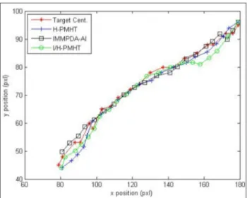
Before submitting the performance results of the tracking process for the inspected scenarios, state estimations of the algorithms and target trajectory for a particular scenario are presented. In this way we aimed to show the tracking perfor-mance after operational improvement and algorithmic amend-ment. Target centroids and estimation trajectories only of oper-ational improvement applied I/H-PMHT, standard H-PMHT and
Table 2. General Summary of the Simulation Scenarios Scenario
Number
No.of Sampling
Frame (Δ) Area (pxlSensor 2)
Area of Air Object
(pxl2)
Mean Velocity
(pxl/frame) (PDIM) (dB)Noise Level SNR (PDIM) (dB) Noise Level (AI) (dB) SNR (AI) (dB)
1 4 250x250 240 2.5 1 8.8 0.84 8.1 2 3 300x300 126 3.8 0.75 8.9 1.17 7.85 3 3 250x250 280 3.3 0 9.89 0.46 8.35 4 2 200x200 78 3 0 8.54 0 6.15 5 2 200x200 88 2.5 0.67 8.3 0.6 5.7 6 3 250x250 40 1.35 0.98 9.74 1.34 6.5 7 3 250x250 434 3.5 1.15 9.93 1.7 7.96 8 2 250x250 450 4.23 0 9.8 0.5 8.26
IMMPDAFAI algorithms throughout the fifth scenario are given in Figure 2. The figures are given for Displayed Cell Threshold (DCT) 5 dB over noise level.
Moreover, in Figure 3 the estimation trajectories were obtained using four iterations for standard H-PMHT and one iteration for I/H-PMHT. In this case I/H-PMHT was subjected to both oper-ational improvements and algorithm amendments, and DCT was selected 5 dB.
The performances of the algorithms are evaluated by hit on the target (HoT), and RMS position estimation error with respect to target centroid. If HoT is greater than 80%, tracking process is as-sumed as successful. After evaluating the performances of the al-gorithms, processing time is taken into account. Processing time is represented with CPU time, and this value is taken as a third
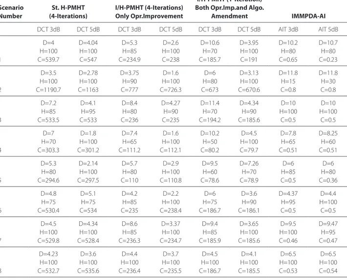
component for evaluation. The processor of the computer used in simulations is Intel-Core i5-3470 CPU with 4 cores at 3.20 GHz. The computer has 4 GB RAM, the OS is Win 7 Professional, and its instruction set is 64-bit. In Table 3 simulation results of algorithms with respect to scenarios are given for evaluation and compari-son. In the table mean values of the algorithms RMS estimation errors with reference to target centroids throughout the scenari-os are given as deviation from target centroid (Dev.Trg.Cent.). Histogram probabilistic multi-hypothesis tracker and I/H-PMHT simulations were conducted for two different Displayed Cell Threshold (DCT) levels, which are 3 dB and 5 dB over noise level. For amplitude information of point measurement data, which is used in IMMPDA-AI simulations, AI Threshold (AIT) levels were also selected 3 dB and 5dB over noise level. A fair comparison was made between the performances of the algorithms. The results obtained in the simulation study are summarized as follows;
- The simulation results show that standard H-PMHT and only operational improvement applied I/H-PMHT both outperform on IMMPDA-AI in terms of estimation error and HoT for whole scenarios. If we compare the results obtained with I/H-PMHT (operational improvement and algorithmic amendment ap-plied) and the results obtained with IMMPDA-AI, they show similar performance for DCT 3 dB over noise level, and I/H-PM-HT shows better performance for DCT 5 dB over noise level. In terms of processing time, IMMPDA-AI is unquestionably supe-rior to the other algorithms. After attempting the operational improvement and algorithmic amendment, I/H-PMHT provides a respectable processing time decrease, but is still not suffi-cient for real-time tracking.
- When only operational improvement is applied, standard H-PMHT gives better results than I/H-PMHT at 3 dB higher level DCT, and worse results at 5 dB higher level DCT. The only excep-tion takes place in the sixth scenario, which has a relatively small object area. These results show that only operational improve-ment applied I/H-PMHT (single scan, multi iteration structure) is more suitable for video object tracking than the standard H-PM-HT algorithm. In this case CPU time reduction is relatively high. - When both operational improvement and algorithmic amend-ment occur standard H-PMHT outperforms I/H-PMHT for 3 dB higher level DCT. On the other hand, for 5 dB higher level DCT the performance of I/H-PMHT is similar to the performance of the standard H-PMHT, and outperforms for high intensity tar-get cases (scenarios 1, 6, 7).
- Using PDIM data with Standard H-PMHT and I/H-PMHT gives satisfactory results, and this shows that PDIM data is suitable for video object tracking.
- When the decreased processing time is taken into account from Standard H-PMHT to only operational improvement ap-plied I/H-PMHT, and both operational improvement and algo-rithmic amendment applied to I/H-PMHT, then the amount of increased or decreased estimation error rate must also be
tak-Figure 2. Target Centroids and State Estimations throughout
Sce-nario 5 (only operational improvement is applied to I/H-PMHT)
Figure 3. Target Centroids and Estimations throughout Scenario
5 (applied both operational improvements and algorithm amend-ment to I/H-PMHT)
en into account. For this purpose, Table 4 was prepared using the results of the simulation study.
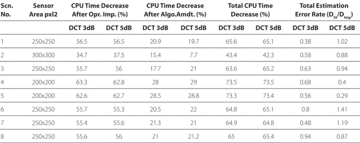
Table 4 shows that a decrease in processing time is directly re-lated to the sensor area. In wider sensor areas processing time decreasing is low, and vice versa. Also converging to target cen-troids with standard H-PMHT occurs rapidly for small sensor ar-eas (scenarios 4 and 5), even if target intensities are not high. I/H-PMHT requires high target intensities, and especially for DCT’s 5 dB higher than noise level has sufficient success. Esti-mation errors of I/H-PMHT obtained for all scenarios are within acceptable limits for track continuation.
Conclusion
This study has provided a new approach for reducing the CPU time of H-PMHT algorithm. For this purpose, operational
im-provement and algorithmic amendment processes were applied to standard H-PMHT algorithm, and I/H-PMHT algorithm was ob-tained. Measurement data used in the study is defined as PDIM data. The PDIM data was obtained from true color video data of flying objects taken from the ground. PDIM data is very useful and easily processed for filtering moving objects from the sta-tionary ones, and for use with H-PMHT and its variations. In the experimental study using PDIM data, standard H-PMHT and operational improvement applied I/H-PMHT and both op-erational improvement and algorithmic amendment applied I/H-PMHT algorithms present satisfactory tracking results. The comparison was made between standard H-PMHT, operational improvement applied I/H-PMHT, and operational improvement and algorithmic amendment applied I/H-PMHT algorithms. Furthermore IMMPDA-AI algorithm was used for comparison purposes. The results show that improvement on processing
Table 3. Overall Performance of Algorithms Scenario Number St. H-PMHT (4-Iterations) I/H-PMHT (4-Iterations) Only Opr.Improvement I/H-PMHT (1-Iteration) Both Opr.Imp.and Algo.
Amendment IMMPDA-AI DCT 3dB DCT 5dB DCT 3dB DCT 5dB DCT 3dB DCT 5dB AIT 3dB AIT 5dB 1 D=4 H=100 C=539.7 D=4.04 H=100 C=547 D=5.3 H=85 C=234.9 D=2.6 H=100 C=238 D=10.6 H=70 C=185.7 D=3.95 H=100 C=191 D=10.2 H=80 C=0.65 D=10.7 H=80 C=0.23 2 D=3.5 H=100 C=1190.7 D=2.78 H=100 C=1163 D=3.75 H=90 C=777 D=1.6 H=100 C=726.3 D=6 H=80 C=673 D=3.13 H=100 C=670.6 D=11.8 H=15 C=0.8 D=11.8 H=30 C=0.8 3 D=7.2 H=85 C=533.5 D=4.1 H=95 C=533 D=8.4 H=80 C=236 D=4.27 H=90 C=235 D=11.4 H=70 C=194.2 D=4.34 H=90 C=185.6 D=10 H=100 C=0.5 D=10 H=100 C=0.5 4 D=7 H=70 C=303.3 D=1.8 H=100 C=301.2 D=7.4 H=65 C=111.2 D=1.6 H=100 C=112.1 D=10.2 H=50 C=80.2 D=4.5 H=100 C=79.7 D=7.8 H=65 C=0.51 D=8.25 H=60 C=0.51 5 D=5.3 H=80 C=294.6 D=2.14 H=100 C=297.5 D=5.7 H=80 C=110 D=2.9 H=100 C=110.8 D=9.5 H=60 C=78.6 D=7.26 H=70 C=78.9 D=6 H=85 C=0.5 D=6 H=80 C=0.36 6 D=4.8 H=75 C=530.4 D=5.1 H=75 C=534 D=4.2 H=85 C=235 D=2.2 H=100 C=238.4 D=6 H=75 C=186.7 D=3.6 H=90 C=186.1 D=4.37 H=95 C=0.5 D=4.4 H=100 C=0.5 7 D=4.5 H=100 C=529.8 D=4.34 H=100 C=528.4 D=8.6 H=85 C=236.3 D=3.37 H=100 C=234.7 D=9.4 H=85 C=185.9 D=3.65 H=100 C=185.6 D=9.5 H=100 C=0.46 D=9.47 H=95 C=0.47 8 D=4.23 H=100 C=532.7 D=3.6 H=100 C=535.6 D=4.4 H=100 C=236.4 D=3.7 H=100 C=235.5 D=4.5 H=100 C=186.7 D=4.1 H=100 C=185.5 D=6.5 H=100 C=0.53 D=6.5 H=100 C=0.54
D: mean deviation from target centroid throughout tracking process (in pixels); H: hit on target-HoT throughout tracking process (%); C: CPU time usage throughout tracking process (in seconds); DCT 3 dB: displayed cell threshold is in the level of 3 db higher than noise level; DCT 5 dB: displayed cell threshold is in the level of 5 db higher than noise level; AIT: amplitude information threshold
time up to 73.5% (with respect to sensor area dimensions) is possible. Also, further reducing the sensor area will result in further decrease in processing time. The tracking performance after improvements is also sufficient for tracking continuity. In this work processing time reduction was achieved, but these results are still not sufficient for real time video tracking. It is assumed that without changing the structure of H-PMHT the lowest CPU time usage border is reached. In the light of these indications future work is planned in which an FPGA based technique in addition to I/H-PMHT will be used in order to achieve real time tracking. In this study only single-target sce-narios have been taken into account, however in some prac-tical circumstances multiple target tracking is required. Also implementing multi-target tracking with I/H-PMHT using PDIM data is another subject for future work.
Peer-review: Externally peer-reviewed.
Conflict of Interest: The author have no conflicts of interest to declare. Financial Disclosure: The author declared that the study has received
no financial support
References
1. S. J. Davey, M. G. Rutten, B. Cheung, “A Comparison of Detection Performance for Several Track-before-Detect Algorithms”, EUR-ASIP J. Adv. Signal Process, 2008.
2. C. Kathirvel, D. Mohanapriya, K. Mahesh, “A Novel Robust Ap-proach for Moving Object Detection and Tracking in Video Sur-veillance System”, IJSRST, vol. 3, no. 8, pp.1235-1241, 2017. 3. X, Dong, J. Shen, D. Yu, W. Wang, J. Liu, H. Huang, “Occlusion-Aware
Real-Time Object Tracking”, IEEE Transactions On Multimedia, vol. 19, no. pp. 763-771, 2017
4. S. S. Blackman, R. Popoli, “Design and Analysis of Modern Tracking Systems”, Artec House, Norwood, MA, USA, 1999.
5. Y. Bar-Shalom, X. R. Li, “Multitarget-Multisensor Tracking: Princi-ples and Techniques”, YBS, Storrs, CT, USA, 1995.
6. R. L. Streit, “Tracking on Intensity-Modulated Data Streams, NU-WC-NPT Technical Report 11.221, Naval Undersea Warfare Center Division” Newport, Rhode Island, USA, 2000.
7. H. X. Vu, S. J. Davey, “Track-Before-Detect using Histogram PMHT and Dynamic Programming, In Digital Image Computing Tech-niques and Applications”, International Conference (DICTA 2012), Fremantle, WA, 2012.
8. M. J. Walsh, M. L. Graham, R.L. Streit, T.E. Luginbuhl, L. E. Mathews, “Tracking on Intensity-Modulated Data Streams, Proceedings of the 2001”, IEEE Aerospace Conference, Big Sky, MT, 2001. 9. R. L. Streit, M.L. Graham, M. J. Walsh, “Tracking in Hyper-Spectral Data,
Information Fusion 2002”, Annapolis, MD, USA, 2002, pp.852-859. 10. A. G. Pakfiliz, M. Efe, “Multi-Target Tracking in Clutter with
Histo-gram Probabilistic Multi-Hypothesis Tracker, In Proc.” IEEE Conf Syst Eng, Las Vegas, USA, pp.137-142, 2005.
11. S. J. Davey, “Histogram PMHT with Particles”, In Proceedings of the 14th International Conference on Information Fusion”, Chicago, Illi-nois, USA, 2011.
12. M. Wieneke, S. J. Davey, “Histogram PMHT with Target Extent Es-timates Based on Random Matrices”, In Proceedings of the 14th International Conference on Information Fusion, Chicago, Illinois, USA, July 2011.
13. Y. Bar-Shalom, T. Kirubarajan, X. Lin, “Probabilistic Data Association Techniques for Target Tracking with Applications to Sonar, Radar and EO Sensors”, IEEE Aerospace and Electronic Systems Magazine, vol. 20, no. 8, pp.37-56, 2005.
14. R. C. Gonzalez, R.E. Woods, “Digital Image Processing. 2nd ed. Pren-tice Hall, New Jersey (USA), 2002.
15. A.J. Lipton, H. Fujiyoshi, R. S. Patil, “Moving target Classification and Tracking from Real-Time Video”. Proc of Workshop Applications of Computer Vision, Princeton, New Jersey, USA, pp. 129-136, 1998. 16. C. Stauffer, W. Eric, L. Grimson, “Learning Patterns of Activity Using
Real-Time Tracking”. IEEE Transactions on Pattern Analysis and Ma-chine Intelligence, vol. 22, no. 8, pp. 747-757, 2000.
Table 4. Offset Compromise between Processing Time and Performance of Standard and Improved H-PMHT Algorithms Scn.
No. Area pxl2Sensor CPU Time Decrease After Opr. Imp. (%) After Algo.Amdt. (%)CPU Time Decrease Total CPU Time Decrease (%) Error Rate (DTotal Estimation St/DImp)
DCT 3dB DCT 5dB DCT 3dB DCT 5dB DCT 3dB DCT 5dB DCT 3dB DCT 5dB 1 250x250 56.5 56.5 20.9 19.7 65.6 65.1 0.38 1.02 2 300x300 34.7 37.5 15.4 7.7 43.4 42.3 0.58 0.88 3 250x250 55.7 56 17.7 21 63.6 65.2 0.63 0.94 4 200x200 63.3 62.8 28 29 73.5 73.5 0.68 0.4 5 200x200 62.6 62.7 28.5 28.8 73.3 73.4 0.56 0.29 6 250x250 55.7 55.3 20.5 22 64.8 65.1 0.8 1.41 7 250x250 55.4 55.6 21.3 21 64.9 64.8 0.48 1.19 8 250x250 55.6 56 21 21.2 65 65.4 0.94 0.87
DSt: mean deviation of standard H-PMHT (in pixels); DImp: mean deviation of I/H-PMHT-both operational improvement and algorithmic amendment applied (in pixels); Opr. Imp.: operational improvement; Algo. Amdt.: algorithmic amendment
17. Y. Boers, F. Ehlersand, W. Koch, T. Luginbuhland, L. D. Stone, R. L. St-reit, “Track before Detect Algorithms”, EURASIP J Adv Signal Process, 2008.
18. S. J. Davey, H. X. Gaetjens, “Track-Before-Detect Using Expecta-tion MaximisaExpecta-tion: The Histogram Probabilistic Multi-hypothesis Tracker: Theory and Applications”, Springer, Singapore, 2018. 19. S. J. Davey, M. Wieneke, “Tracking Groups of People in Video with
Histogram-PMHT” Defense Apps. of Signal Processing (DSAP) 2011 Workshop, Coolum, Queensland, Australia, 2011.
20. R. L. Streit, T. E. Luginbuhl, “Probabilistic Multi Hypothesis track-ing, Technical Report NUWC-NPT 10,428, Naval Undersea Warfare Center Division”, Newport, Rhode Island, USA, 1995.
21. Y. Bar-Shalom, T.E. Fortmann, “Tracking and Data Association” Aca-demic Press, NY, USA, 1988.
Ahmet Güngör Pakfiliz received his B.S. degree in Electrical Engineering from Yıldız Technical University in 1991, M.S. degree in Electrical and Electronics Engineering from Middle East Technical University in 1997 and Ph.D. degree in Electronics Engineering from Ankara University in 2004. He is currently an Assistant Professor at the Department of Electrical and Electronics Engineering of Başkent University.