Comparison of the forecast performances of linear time series and artificial neural network models within the context of Turkish inflation

TURKISH INFLATION

The Institute of Economics and Social Sciences of

Bilkent University

by

NURİ UÇAR

In Partial Fulfilment of the Requirements for the Degree of

MASTER OF ARTS

in

THE DEPARTMENT OF ECONOMICS BİLKENT UNIVERSITY

ANKARA

I certify that I have read this thesis and have found that it is fully adequate, in scope and in quality, as a thesis for the degree of Master of Arts in Economics.

...

Assoc.Prof. Serdar SAYAN Supervisor

I certify that I have read this thesis and have found that it is fully adequate, in scope and in quality, as a thesis for the degree of Master of Arts in Economics.

... Assoc.Prof. Dilek Önkal Examinig Committee Member

I certify that I have read this thesis and have found that it is fully adequate, in scope and in quality, as a thesis for the degree of Master of Arts in Economics.

...

Assoc.Prof. Kıvılcım Metin Özcan Examinig Committee Member

Approval of the Institute of Economics and Social Sciences

... Prof. Dr. Kürşat Aydoğan Director

iii

A COMPARISON OF THE FORECAST PERFORMANCES OF LINEAR TIME SERIES AND ARTIFICIAL NEURAL NETWORK MODELS WITHIN THE CONTEXT OF

TURKISH INFLATION

Uçar, Nuri

M.A., Department of Economics Supervisor: Assoc. Prof. Dr. Serdar Sayan

October 2001

This thesis compares a variety of linear and nonlinear models to find the one with the best inflation forecast performance for the Turkish Economy. These comparisons are performed by considering the type of series whether or not stationary. Different combination techniques are applied to improve the forecasts. It is observed that the combination forecasts based on nonstationary vector autoregressive (VAR) and artificial neural network (ANN) models are better than the ones generated by other models. Furthermore, the forecast values combined with ANN technique produce lower root mean square errors (RMSE) than the other combination techniques.

iv

DOĞRUSAL ZAMAN SERİLERİ VE YAPAY SİNİR AĞLARI MODELLERİNİN ÖNGÖRÜ PERFORMANSLARININ TÜRKİYE’DEKİ ENFLASYON BAĞLAMINDA

KARŞILAŞTIRILMASI

Uçar, Nuri

Yüksek Lisans, İktisat Bölümü Tez Yöneticisi: Doç.Dr. Serdar Sayan

EKİM 2001

Bu çalışma, Türk ekonomisi için en iyi öngörü performansına sahip doğrusal ve doğrusal olmayan modelleri karşılaştırmaktadır. Bu karşılaştırma serilerin durağan ve durağan olmama durumları dikkate alınarak gerçekleştirilmiştir. Durağan olmayan vektör otoregresif ve Yapay Sinir Ağları (YSA) modellerinden elde edilen öngörülerin birleştirilmesi, diğer modellere göre daha başarılı olmuştur. Ayrıca, YSA tekniği ile birleştirilen öngörüler diğer birleştirme tekniklerine göre daha küçük hatalar vermiştir.

v

TABLE OF CONTENTS

ABSTRACT ... iii ÖZET ... iv TABLE OF CONTENTS... v CHAPTER 1: INTRODUCTION... 1

CHAPTER 2: LITERATURE REVIEW... 4

CHAPTER 3: STATISTICAL PROPERTIES OF LINEAR TIME SERIES AND ARTIFICIAL NEURAL NETWORK MODELS... 8

3.1 Linear Models... 8

3.1.1 Univariate Time SeriesModels:Box-Jenkins Approach... 8

3.1.2 Multivariate Time Series Models... 13

3.2 Nonlinear Models... 15

3.2.1 Exponential Trend Model (ETREND)... 15

3.2.2 Artificial Neural Network Approach... 15

CHAPTER 4: EMPIRICAL RESULTS... 20

4.1 The Data... 20

4.2 The Forecasting Models: Specification and Estimation... 23

4.2.1 Box-Jenkins Modelling ... 23

4.2.2 Vector Autoregressive (VAR) Model... 24

4.2.3 Neural Network Models... 26

4.2.4 The Exponential Trend Model (ETREND)... 28

4.3 Forecasting Performance Evaluation... 29

4.4 The Combination of Forecasts... 31

CHAPTER 5: CONCLUSIONS... 35

1

CHAPTER 1

INTRODUCTION

This thesis aims to compare forecast performances of conventional linear models to non-linear alternatives including artificial neural networks. The use of forecasting techniques employed is illustrated in reference to inflation forecasts for Turkish economy which has experienced high levels of inflation over the last two decades.

Although the yearly inflation was over 100 percent in certain years during this period, hyperinflationary levels were not reached. Many unsuccessful disinflationary programs have been implemented in this period. Average annual inflation rate reached 35-40 percent in the early 1980’s, 60-65 percent in the late 1980s and was around 80 percent before the Turkish government started another disinflationary program under the guidance of IMF July 1998. The Russian crisis in August 1998, general elections in April 1999 and the two earthquakes in August and October 1999 were among the factors contributing to the governments’ failure to curb the inflation rate and eliminate fiscal imbalances (Ertuğrul and Selçuk, 2001).

The new government started implementing its “exchange rate based stabilization program” at the beginning of the year 2000. The aim of the program was to achieve a considerable reduction in the inflation rate from its current level of 60-70 percent per year to single digits by the end of year 2002. The main tool of this program for the achievement of inflation targets was a preannounced crawling peg. However, Turkey faced another crisis in February 2001 which led to the collapse of preannounced crawling peg regime. Turkey then switched from crawling peg to the floating exchange rates. Today, the government prepares the program to implement a new inflation targeting program under the floating exchange rate

2

regime. Thus, accurate forecasting is important to foresee the future path of inflation.

Specification and estimation of linear time series models are well-established procedures, based on ARIMA univariate models or multivariate VAR type models. However, economic theory frequently suggests nonlinear relationships between variables and many economists believe that the economic system is nonlinear. Moreover, most of the recent work in time series analysis has been done on the assumption that the structure of the series can be described by linear time series models. However, there are some cases for which theory and data suggest that linear models are unsatifactory. To investigate the validity of this argument in the context of Turkish inflation, this thesis considered nonlinear models along side linear forecasting models. Another objective of the thesis is to analyse both stationary and nonstationary approaches in order to examine the importance of the type of series used for the forecasting ability of competing models. Hence, considerable emphasis has been placed on the selection of models and seires to obtain best out-of-sample forecasts. This has been done with real data inflation and exchange rate. Different combinations of forecast results are considered to improve the forecasts of each model. The following chart summarizes alternative models and the types of series considered.

MODELS

Linear Models Nonlinear Models

Univariate Multivariate Neural Network ExpTrend

Stationary Stationary Nonstationary Stationary Nonstationary Nonstationary

3

The discussion in the rest of the thesis is organised as follows. Chapter 2 contains a literature review. Chapter 3 describes the mathematical properties of the models and forecasting methods used. Chapter 4 reports the forecasting results obtained through the application of models to Turkish inflation, and discusses their implications. Chapter 5 concludes the thesis by comparing the methods in the light of results.

4

CHAPTER 2

LITERATURE REVIEW

This chapter reviews the literature on the forecasting of time series with Artificial Neural Network (ANN) and the statistical time series . We briefly discuss the results of these studies by paying particular attention to the forecasting performances of ANN and conventional methods (linear and nonlinear time series models) considered in these articles.

Neural networks and traditional time series techniques have been compared in several studies. Some of these studies are interested only in the forecasting performances of ANN models in comparison to traditional approaches. Foster, et.al. (1991) and Sharda and Patil (1990, 1992) have used a large data set from the well-known “M-competition” in Makridakis, et.al. (1982). Foster, et.al. (1991) found neural networks to be inferior to the least squares statistical models for time series of yearly data. However, Sharda and Patil (1992) and Tang, et.al. (1991) agreed that for a large number of observations, ANN models and Box-Jenkins models produce comparable results. Kang (1991) observed using 18 different neural network architectures that the forecast errors are lower for the series containing trend and seasonal patterns. He also concluded that neural networks often performed better for the long horizon forecast periods. On the other hand, Hill, et.al. (1996) produced forecasts by neural networks and compared with the forecasts from neural networks to those obtained by Makridakis, et.al. (1982). They have arrived at the conclusion that neural networks did significantly better than traditional methods for monthly and quarterly series. In additon, they suggested that selecting

5

the best neural network architecture with fewer parameters to be estimated is crucial to successful neural network modeling.

Kohzadi, et.al. (1996) carried out an empirical investigation comparing artificial neural network and time series models. They constructed an ARIMA model and compared it to an ANN model in terms of forecasting performance. They also made a comparison to determine which model caught the turning point of the series. They reached the conclusion that neural network models were able to capture a significantly more turning points as compared to the ARIMA model. Furthermore, they have made a very controversial point by stating that “The neural network with only one hidden layer can precisely and satifactorily approximate any continuous function” (Kohzadi, et.al., 1996, p.179).

However, Adya and Collopy (1998) have evaluated the effectiveness of forecasting with ANN by taking 48 articles published between 1988 and 1994 into consideration. Some of these studies produced contradicting results to the statement by Kohzadi, et.al. (1996) indicating that real-world data may not always be consistent with the theoretical implications. Simulation experiments have to be used to verify what the theory says instead of departing from real world observations.

Although much of the literature in the emerging field of ANN is focused on modelling time series data and making forecast performance comparisons between competing models, Gorr, et.al. (1994) have employed cross section data to predict student grade point averages by comparing linear regression and stepwise polynomial regression versus ANN structure. They found that mean errors of the model forecasts were not comparable, implying that no model was superior to the others. They have explained these results by the neural network structure. However, it may be argued that another reason might be their use of qualitative variables in

6

the models. Since the only values these variables take are zeros and ones, ANN learning mechanism does not work well due to the large numerical distinction in the observations of qualitative and quantitative variables.

A few studies investigate the effect of the stationarity on the forecasting performance of the ANN and traditional time series models. Lachtermacher and Fuller (1995) have studied both stationary and nonstationary data and constructed an ARMA model via Box-Jenkins methodology to be compared against an ANN model for four annual river flows. They observed that neural network models outperformed the ARIMA model and the improvements of the forecast values in the nonstationary case were much larger than in the stationary case. This is consistent with the study of Tang, et.al. (1991). On the other hand, Nelson, et.al. (1999) emphasized the effect of seasonality on the forecasting of time series. They have compared ANN forecasts with Box-Jenkins forecasts.Their results indicate that when there is seasonality in the time series, forecasts from neural networks estimated on deseasonalized data get significantly more accurate than the forecasts produced by neural networks that were estimated using data which were not deseasonalized.

Accurate prediction of macroeconomic variables is problematic and many of the linear models that have been developed perform poorly. In recent years, it has been widely agreed that many macroeconomic relations are nonlinear and neural networks can model linear and nonlinear relationships among variables as well as nonlinear econometric modelling. Yet, there has been little work on forecasting macroeconomic time series using the ANN models and comparing alternative structural and time series econometric models via forecast performance criteria. Maasoumi, et.al. (1994) applied an ANN model to forecast some US macroeconomic series such as the Consumer Price Index, unemployment, GDP, money and

7

wages. Their work does not include any comparison because they produced only in sample forecasts with the ANN model. They interpret the in sample results which failing to show the prediction power of ANN model examined in their study.

On the other hand, Swanson and White (1997) applied an ANN model to forecast nine US macroeconomic series and compared their results with those from traditional econometric approaches. The results are mixed, but Swanson and White concluded that ANN models have good forecast performance relative to the traditional models even when there is no explicit evidence for nonlinearity. Moshiri and Cameron (2000) have used ANN modelling technique and compared the results with the traditional econometric approaches to forecast the inflation rate. Their results showed that ANN models are able to forecast as well as the traditional econometric methods examined and to outperform them in some cases.

The literature suggests several mathematical advantages of neural networks have over traditional statistical methods. Neural networks have been shown to be universal approximators of functions (Cybenko, 1989; Funahashi, 1989) and their derivatives (White, et.al., 1992) . They can also be shown to approximate ordinary least squares regression (White and Stinchcombe, 1992) , nonparametric regression (White, et.al., 1992) and Fourier analysis (White and Gallant, 1992). Hence, neural networks can approximate whatever functional form best characterizes a time series implying that standard asymptotic theory can be appropriately applicable to the nonlinear functional structure of ANN.

8

CHAPTER 3

STATISTICAL PROPERTIES OF LINEAR TIME SERIES

AND ARTIFICIAL NEURAL NETWORK MODELS

This chapter discusses statistical properties of time series and ANN techniques used in the empirical analysis in the following chapter. This chapter first explains statistical properties of univariate and multivariate linear time series models used in the thesis. Then, the characteristics of nonlinear models considered are described. These are exponential trend model and artificial neural network model, as shown in Figure 1.

3.1 Linear Models

This section deals with statistical properties of univariate and multivariate (vector) time series models.

3.1.1 Univariate Time Series Models: Box-Jenkins Approach

A time series is an ordered sequence of observations, and a realization or sample function from certain stochastic process. Many economic time series have such characteristics as a trend which represents the long-run movements in the series, and a seasonal pattern which regularly repeats over a certain time interval. Hence, a model of the series will need to capture these characteristics. There are basically two reasons for modelling the time series. The first is to provide a description of the series in terms of its components of interest. One

9

may want to examine the trend to see the main movements in the series or be interested in the seasonal behaviour of the series. The second is to underlie the construction of a univariate time series model is the desire to the predict the future course of the series.

The rest of this section introduces the definitions of basic concepts used within the context of forecasting with univariate autoregressive model, and describes the forecasting process itself.

A time series is said to be strictly stationary if the joint distribution of

X ,...,

_t1

X

_tnhas the joint distribution

X

_t1+p

,...,

X

_tn+p

∀

p

;

∀

t

_i

,

i

=

1

,...,

n

.

More explicitly, the distribution of the stationary process remains unchanged when evolved in time by an arbitrary value p. Moreover, the n-dimensional distribution function

F

(

X

_t1

,...,

X

_tn

)

is said to be first-order stationary in distribution if its one dimensional distribution function is time invariant, i.e,

)

(

)

(

X

_t1

F

X

_{t1 p}

F

=

₊ for any integers

t

_1,

t

_1+pand p. This can be extended to the higher order stationarity. For instance, the nth order stationary in distribution can be represented as

(

F

X

_t1

,...,

X

_tn

)

=

F

(

X

_t1+p

,...,

X

_tn+p

)

for any n-tuple

t ,...,

₁

t

_n and p of integers.

The concept of stationarity is defined in terms of movements rather than in terms of the distribution function. For a given process

X

_t mean function of the process will be

)

(

_t t

=

E

X

µ

, the variance of the process

σ

2

=

E

(

X

_t

−

µ

_t

)

2and the covariance function between

X

_t1and

X

_t2 is such that

Cov

(

X

_t1,

X

_t2

)

=

Cov

(

X

_{t1 p+}

,

X

_{t2 p+}

)

=

γ

_p where

p

t

t

₁

−

₂

=

. The mean and variance of

X

_t depend only on the lag p . Thus, the process

X

_t

is said to be weak or covariance stationary. For a stationary process

X

_t , the correlation between

X

_t and

X

_t+p will be:

10 0

)

(

)

(

)

,

(

γ

γ

ρ

p p t t p t t p

X

Var

X

Var

X

X

Cov

=

=

+ + (3.1)

where

Var

(

X

_t

)

=

Var

(

X

_{t+ p}

)

=

γ

₀.

γ

_p is called the autocovariance function and

ρ

_pis called the autocorrelation function (ACF) in time series analysis since they represent the covariance and correlation between

X

_t and

X

_t+p from the same process, seperated only by p time lags. In addition, someone may wish to investigate the correlation between

X

_t and

p t

X

₊ after mutual linear dependence on the intervening variables

X

_t+1

,...,

X

_t+p−1 has been removed. This is known as partial autocorrelation analysis in the time series literature. If

Xˆ

_t and

X

ˆ

_t+p are the best linear estimate of

X

_t and

X

_t+p , respectively, then the partial autocorrelation can be defined as follows:

[

]

)

(

)

(

ˆ

,

(

),

ˆ

,

(

p t t p t p t t t p

X

Var

X

Var

X

X

X

X

Cov

P

+ + +

=

(3.2)

Suppose that

ε

_t is a purely random process with mean zero and variance

σ

2. Then, the process given by

X

_t

=

φ

₁

X

_t−1

+

φ

₂

X

_t−2

+

...

+

φ

_p

X

_t−p

+

ε

_t is called an autoregressive process of order p and is denoted by AR(p). Using the lag operator L, AR(p) can be written as:

φ

(

L

)

X

_t

=

ε

_t where

φ

(

L

)

=

1

−

φ

₁

L

−

...

−

φ

_p

L

p. To be stationary, the roots of

0

)

(

L

=

p

φ

must lie outside the unit circle. The first order autoregressive process can be written as:

(

1

−

φ

₁

L

)

X

_t

=

ε

_t and for it to be stationary, the root of

(

1

− L

φ

₁

)

=

0

must be outside of the unit circle. That is, for a stationary process, we have

φ

₁

〈

1

. The autocovariances are obtained as follows :

11

)

(

)

(

)

(

X

_{t p}

X

_t

E

₁

X

_{t p}

X

_{t 1}

E

X

_{t p t}

E

₊

=

φ

_{− −}

+

₋

ε

(3.3) or

γ

_p

=

φ

₁

γ

_p−1

,

p

≥

1

(3.4)

and the autocorrelation function becomes

ρ

_p

=

φ

₁

ρ

_p−1

=

φ

₁

p

,

p

≥

1

where use is made of the fact that

ρ

₀

=

1

. Since

φ

₁

〈

1

, the ACF exponentially decays depending on the sign of

1

φ

. The PACF of the AR(1) process shows a positive or negative spike at lag 1 depending on the sign of

φ

₁, and then cuts off for other lags.

On the other hand, autocovariance of p-th order autoregressive process can be obtained by multiplying both sides of AR(p) process with

X

_t−k:

t k t p t k t p t k t t k t

X

X

X

X

X

X

X

₋

=

φ

_{1 − −1}

+

...

+

φ

_{− −}

+

₋

ε

(3.5)

and taking the expected value yields

γ

_k

=

φ

₁

γ

_k−1

+

...

+

φ

_p

γ

_k−p

,

k

〉

0

where

0

)

.

(

X

_{t−k t}

=

E

ε

for

k

〉

0

. So,

ρ

_k

=

φ

₁

ρ

_k−1

+

...

+

φ

_p

ρ

_k−p

,

k

〉

0

is the autocorrelation function which has the recursive relationships.

One of the most important issues in the analysis of a time series is to forecast its future values. Since the early 1980s the use of stationary linear autoregressive models has become widespread in econometrics for analysing and forecasting time series data.

Suppose someone needs to forecast variable

Y

_t+τ based on a set of variables

X

_t observed at date t. Assume that

X

_t consists of m-past values of

Y

_t+τ such as

Y

_t

,

Y

_t−1

,...,

Y

_t−m+τ. Let

1

ˆ

₊ t

Y

denote a forecast of

Y

_t+1 based on

X

_t. Then,the quadratic loss function can be used to evaluate the forecasts which have the minumum errors. This can be specified as:

2

)

ˆ

(

Y

_t+τ

−

Y

_t+τ

12

forecast

Yˆ

_t+τand denoted

MSE

(

Y

ˆ

_t+τ

)

≡

E

(

Y

_t+τ

−

Y

ˆ

_t+τ

)

2. Moreover, the smallest mean square error achieved for the one step ahead forecast since the forecast of

Y

_t+1 is equivalent to the expectation

Y

_t+1 conditional on

X

_t such that

Y

ˆ

_t+1

=

E

(

Y

_t+1

X

_t

)

(Hamilton, 1994).

Now, it is convenient to show the derivation of minumum MSE forecast for AR(1) model used in the empirical part of this study. Consider the stationary AR(1) model with drift :

)

,

0

(

,

_t 2 1 1

ε

ε

σ

φ

Y

iidN

c

Y

_t

=

+

_t−

+

_t

≈

. Since it is stationary , it can be defined in terms of moving average (MA) model. Thus ,

t t t t

L

c

c

Y

ε

θ

ε

θ

ε

)

(

..

1 1

+

=

+

+

+

=

₋ (3.6) where

∑

∞ = −

₌

−

=

0 1 1

)

1

(

)

(

j j j

L

L

L

φ

θ

θ

. For the

τ

periods ahead, we have the following:

∑

∞ = − + +

=

+

0 j j t j t

c

Y

_τ

θ

ε

_τ (3.7)

The minimum mean square error forecast

Yˆ

_t+τ of

Y

_t+τ can be imposed as:

...

ˆ

ˆ

ˆ

_t+

₌

_c

₊

_t

₊

_{+1 t−1}

₊

Y

_τ

θ

_τ

ε

θ

_τ

ε

(3.8)

where

θ

ˆ

_τ are parameters to be determined . Hence, the mean square error of the forecast is :

[

]

2 0 2 1 0 2 2 2

_ˆ

)

ˆ

(

∑

∑

∞ = + + − = + +

−

=

+

−

j j j j j t t

Y

Y

E

_{τ τ} τ τ τ

σ

θ

σ

θ

θ

(3.9)

and by setting

θ

_j+τ

=

θ

ˆ

_j+τ. More explicitly, mean square

τ

period ahead forecast error becomes

[

1

+

φ

2

+

φ

4

+

...

+

φ

2(τ −1)

]

σ

2 .

13

3.1.2 Multivariate Time Series Models

In dealing with economic variables, the value of the variable is typically related not only to its predecessors in time but also depends on past values of other variables. For instance, household consumption expenditures may depend on variables such as income, interest rates and investment expenditures. If all these variables are related to the consumption expenditures it makes sense to use their possible additional information content in forecasting consumption expenditures (Lütkepohl, 1993).

Denoting the relevant variables by

Y

_1t

,

Y

_2t

,...,

Y

_Kt , the forecast of

Y

_1,T+τ may be of the functional form:

Y

_1,T+τ

=

g

₁

(

Y

_1,T

,

Y

_2,T

,...,

Y

_K,T

,

Y

_1,T−1

,...,

Y

_K,t−1

,

Y

_1,T−2

,...)

. Similarly a forecast for the second variable may depend on the past values of all varaiables in the system. More generally,

,...)

,

,...,

,

,...,

,

(

ˆ

2 , 1 1 , 1 , 1 , , 2 , 1 ,T+

=

K T T K T T− K t− T− K

g

Y

Y

Y

Y

Y

Y

Y

_τ (3.10)

A set of time series

Y

_KT

,

k

=

1

,...,

K

and

t

=

1

,...,

T

is called a multivariate time series and τ

+ T K

Y

ˆ

_, indicates the forecast as a function of multivariate or vector time series.

Forecasting is one of the main objectives of vector time series analysis. The forecaster tries to make predictions in a particular period t about the future values of variables . In order to make forecasts, he has a model which explains data generation process and an information set containing the available information in period t.

Vector generalization of univariate autoregression denoted VAR(p) can be written as follows: t p t p t t t

c

Y

Y

Y

Y

=

+

φ

_{1 −1}

+

φ

_{2 −2}

+

...

+

φ

₋

+

ε

(3.11)

14

where

Y

_t

=

(

Y

_1t

,...,

Y

_KT

)

′

is a (Kx1) random variables vector,

φ

_i are fixed (KxK) coefficient matrices ,

c

=

(

c

₁

,...,

c

_K

)

′

is a fixed (Kx1) vector of intercept terms allowing for the possibility of a nonzero mean

E

(

Y

_t

)

. Finally,

ε

_t

=

(

ε

_1t

,...,

ε

_Kt

)

′

is a K-dimensional white noise, that is ,

E

(

ε

_t

)

=

0

,

E

(

ε

_t

ε

′

_t

)

=

Ω

and

E

(

ε

_t

ε

_τ

′

)

=

0

for

t

≠

τ

.

Let us consider a zero mean VAR(1) process :

Y

_t

=

φ

₁

Y

_t−1

+

ε

_t . This can be written in MA form by taking

τ

- ahead forecast horizon into consideration:

∑

− = − + +

=

+

1 0 1 1 τ τ τ τ

φ

φ

ε

i i t i t t

Y

Y

(3.12)

Moreover, forecast of

Y

_t+τ is the linear VAR(p) process described:

...

1 1 0

+

+

=

₋ + t t t

A

Y

A

Y

Y

_τ (3.13)

where the

A

_i are (KxK) coefficient matrices , we get the following forecast error is given by:

∑

∑

∞ = − − = − + + +

−

=

+

−

−

1 0 1 1 0 1

(

)

ˆ

i i t i t i i t i t t

Y

A

Y

A

Y

Y

τ τ τ τ τ

φ

ε

φ

(3.14)

MSE is obtained through multiplication of this equation with its transpose and application of expectation operator, resulting in the following :

1 1 1

ˆ

+ − +τ

=

φ

τ t

=

φ

t τ t

Y

Y

Y

(3.15)

This optimal MSE predictor is used for measuring the forecast performance of VAR(p) process.

15

3.2 Nonlinear Models

This section explains the nonlinear models used in the empirical part, namely Artificial Neural Network Model and Exponential Trend Model.

3.2.1 Exponential Trend Model (ETREND)

This model was first proposed by Gallant (1975) as the type of nonlinear regression model. Exponential trend model is convenient to model variables that follow an exponential path over time. It has the following form:

t

t

T

Y

=

α

₁

exp(

α

₂

)

+

ε

(3.16)

where

Y

_t is dependent variable. In order to acquire reliable estimates with that model, autocorrelation has to be removed by applying autoregressive transformation. For instance, by implementing the AR(1) transformation, we arrive at the following:

[

]

{

_t

}

_t

t

T

Y

T

Y

=

α

₁

exp(

α

₂

)

+

β

_{1 −1}

−

α

₁

exp

α

₂

(

−

1

)

+

ε

(3.17)

This regression is estimated by nonlinear least squares. Making a forecast with this model requires following the same procedure as the linear regression equation.

3.2.2 Artificial Neural Network Approach

Cognitive scientists have proposed a class of flexible nonlinear models inspired by certain features of the way that the brain processes information. Because of their biological inspiration, these models are referred to as artificial neural networks (ANN).

16

ANNs are a class of flexible nonlinear regression and discriminant models, data reduction models and nonlinear dynamical systems. Many ANN models resemble to popular statistical techniques such as generalized linear models, polynomial regression, nonparametric regression and discriminant analysis and so forth. ANNs have the ability of learning through a process of trial and error that can be resembled to statistical estimation of model parameters. An ANN can

(i) automatically transform and represent complex and highly nonlinear relationships (ii) automatically detect different states of phenomena through independently variable patterns.

Hence, ANNs are appropriate for complex phenomena for which we have good measures but a poor understanding of the relationships within these phenomena. Moreover, because of their flexibility and simplicity, usefulness in modelling any type of parametric or nonparametric process and their capacity to automatically handle nonlinearities, ANNs are ideally suited for prediction and forecasting particularly in the cases where linear models fail to perform well.

The ANN consists of basic units, termed neurons, whose design is suggested by their biological counterparts. The neuron combines the inputs, incorporates the effect of bias and outputs signals. In artificial neurons, learning occurs and alters the strength of the connections between the neurons and biases (Hill, et.al, 1994).

In an ANN, a neuron input path i has a signal, xi , on it, i.e., input variable, and the strength

of the path is characterized by a weight ,wi. The neuron is modelled by summing each weight

times the input variable over all paths and adding the node bias

(

θ

)

. This can be expressed as:

17

and it is transformed into output Y with the sigmoid shaped logistic function shown as the following:

)

1

/(

1

+

−Σ

=

e

Y

(3.19)

This S-shaped function shrinks the effect of extreme input values on the performance of the network.

The ANN literature refers to the estimation of unknown parameters as learning. Learning occurs through the adjustment of the path weights and node biases. The most common method used for the adjustment is backpropagation. It is a quasi-gradient method where the parameters are updated after presentation of each observation. Adjusting or updating the parameters after each observation is sometimes called recursive least squares. This technique is based on minimizing the squared difference between the model output and the desired output for an observation in the data set. The squared error is then propogated backward through the network and used to adjust the weigths and biases. The neuron has the following functional form:

∑∑

−

=

i j j i j i

d

y

E

(

1

/

2

)

(

_{, ,}

)

2 (3.20)

where j is an index over the data set used for training the network, i is an index over the output units of the network, y is the actual output unit and d is the desired output unit for that set of inputs.

Back propagation network models may be static or feedforward. In feedforward networks, input vectors are fed into the network to generate output vectors, with no feedback to input vectors again). Moreover, the learning is supervised ( an input vector and a target output vector both are defined and the networks tend to learn the relationship between them through

18

a specified learning rule) (Moshiri and Cameron, 2000 ).

A specific learning rule commonly used in the backpropogation model is the generalized delta rule, which updates the weight for each unit as follows:

∇

+

=

+ i

η

i

w

w

₁ (3.21)

where

w

_i is the weight,

η

is the learning rate (less than 1) and

∇

is the gradient vector associated with the weights. The gradient vector is the set of derivatives for all weights with respect to the output error.

In a general form, the ANN output vector generated by a model or network including p input units, q hidden units (neurons) and one output unit can be written in the functional form as:

∑

=

′

+

′

=

q i i f

x

w

Y

O

1

β

(3.22)

where

O

_f is the final output, Y is the nonlinear transformation function,

x

=

(

x

₁

,...,

x

_p

)

is the input vector ,

w

=

(

w

₁

,...,

w

_q

)

and

β

_i are the weights vectors. Each term of

w

stands for a px1 vector of weights relating to the p input variables.

β

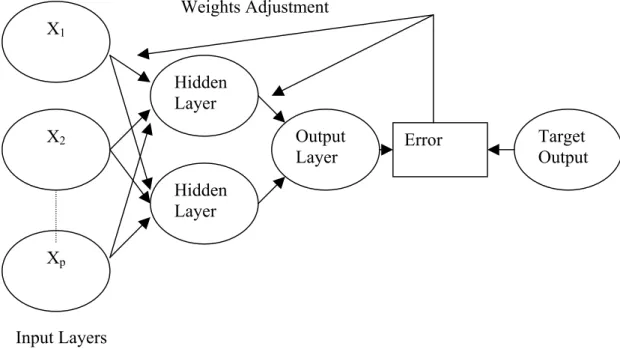
_i refers to a qx1 vector of weights relating each sigmoid function.

Figure 2 gives a sketch of the stages of typical backpropagation neural network model with p inputs, two hidden units and one output unit.

19

Weights Adjustment

.

Input Layers

Figure 2. General Architecture of Back Propagation Neural Network

The working mechanism of backpropagation ANN shown in Figure 2 can be explained in the following steps:

STEP 1. Input and Output vectors are entered into the system. STEP 2. Network assigns parameters to the inputs randomly.

STEP 3. Calculate errors between its predicted outputs and actual outputs. STEP 4. Adjust parameters in the direction required to reduce errors.

STEP 5. Learning process continues until the network reaches a specified error.

X2 Xp Hidden Layer Hidden Layer Output

Layer Error Target Output X1

20

CHAPTER 4

EMPIRICAL RESULTS

This chapter is organized as follows. In the first section, the data set employed is described. In the second section, competing models considered are described. In the third section, we compare the forecasting performances of these models via mean errrors (ME) and root mean square errors (RMSE). The last section of the chapter discusses possible strategies for improving the out of sample forecasts.

4.1 The Data

The data employed are made up of monthly series covering the period between January 1982 and June 2001. The variables examined in this study are described as the following:

TEFE: Wholesale Price Index USD: Exchange rate (TL/USD)

The variable USD is chosen as the only explanatory variable for the inflation in order to avoid the negative effect of the over parametrization on the forecasting performances.

The following graphs of the variables depict the behaviour of each series over time. Figures 3 and 4 show the level of TEFE and USD having an exponential trend for the whole period under consideration. Figures 5 and 6 display the log level of the series denoted LTEFE and LUSD with a strong linear upward trend. The first difference series DLUSD and DLTEFE are plotted in Figures 7 and 8. One can observe the spikes in the April of 1994 when , following a crisis , Turkish Lira significantly depreciated against the US dollar.

21 0 40000 80000 120000 160000 84 86 88 90 92 94 96 98 00 TEFE 0 200000 400000 600000 800000 1000000 1200000 1400000 84 86 88 90 92 94 96 98 00 USD 2 4 6 8 10 12 84 86 88 90 92 94 96 98 00 LTEFE 4 6 8 10 12 14 16 84 86 88 90 92 94 96 98 00 LUSD -0.1 0.0 0.1 0.2 0.3 84 86 88 90 92 94 96 98 00 DLTEFE -0.1 0.0 0.1 0.2 0.3 0.4 0.5 84 86 88 90 92 94 96 98 00 DLUSD

22

The order of integration is investigated for the variables via the Perron-Augmented Dickey Fuller (ADF) test (1989) . Accordingly, the following regression equation is estimated :

t t t

t

c

y

D

u

y

=

+

ρ

₋₁

+

δ

+

(4.1)

where

y

_t

=

(

LUSD

,

LTEFE

)

and

D

_t is the dummy variable which is defined as:







=

=

otherwise

,

0

1994

April

t

,

1

t

D

(4.2)

The following hypothesis is constructed:

1

1

:

1 0

〈

=

=

ρ

ρ

H

H

(4.3)

This is known as the unit root-test. If H0 is not rejected, the previous regression is repeated for

the first difference series to check again whether or not unit root (H0) exists.

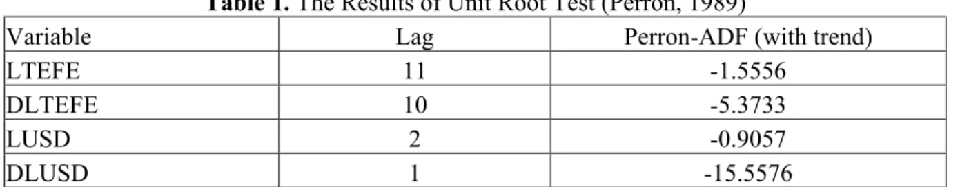
Table 1 reports the results obtained through Perron ADF test. Note that the test was performed with Campbell and Perron (1991) approach, which performs a test starting from the lag 12, and ending with the minimum Akaike Information Criteria (AIC) value, for choosing lag lengths. It is concluded that the integrated order of the series is one. In other words, the series are first difference stationary.

Table 1. The Results of Unit Root Test (Perron, 1989)

Variable Lag Perron-ADF (with trend)

LTEFE 11 -1.5556

DLTEFE 10 -5.3733

LUSD 2 -0.9057

DLUSD 1 -15.5576

Asterisk indicates rejection at the %1 critical value λ=0.56≅0.6 and Perron critical value is –4.45 for α=0.01

23

4.2 The Forecasting Models: Specification and Estimation

This part examines the estimation and specification of the models applied to Turkish inflation.

4.2.1 Box-Jenkins Modelling

The ARMA class of models remain arguably the most popular set of models for economic applications due, possibly, to their relative ease of computation and their ability to produce at least reasonable forecasts across a diverse set of data types.

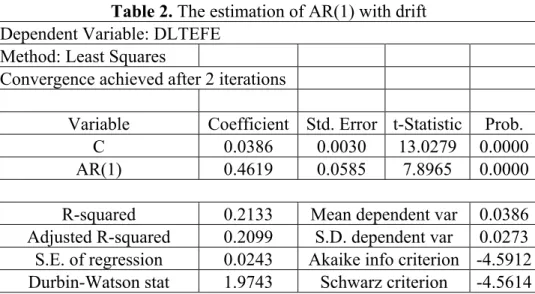
It is well known that post sample forecasting performance of pure AR models usually at least matches those of more complex ARMA models. This is the position taken in this study. Time series data for inflation is modelled with Box-Jenkins methodology. We have analysed the correlograms of the inflation data both in log level and first difference of the log level. A diagnostic test known as Q-statistic has been performed to see whether autocorrelation is removed. It is found that the appropriate model for the inflation series is AR (1) with drift. That is :

t t

t

c

DLTEFE

u

DLTEFE

=

+

β

₋₁

+

(4.4)

24

Table 2. The estimation of AR(1) with drift

Dependent Variable: DLTEFE Method: Least Squares

Convergence achieved after 2 iterations

Variable Coefficient Std. Error t-Statistic Prob.

C 0.0386 0.0030 13.0279 0.0000

AR(1) 0.4619 0.0585 7.8965 0.0000

R-squared 0.2133 Mean dependent var 0.0386 Adjusted R-squared 0.2099 S.D. dependent var 0.0273 S.E. of regression 0.0243 Akaike info criterion -4.5912 Durbin-Watson stat 1.9743 Schwarz criterion -4.5614 The coefficients given in Table 4 are used for the out-of- sample forecasts.

4.2.2 Vector Autoregressive (VAR) Models

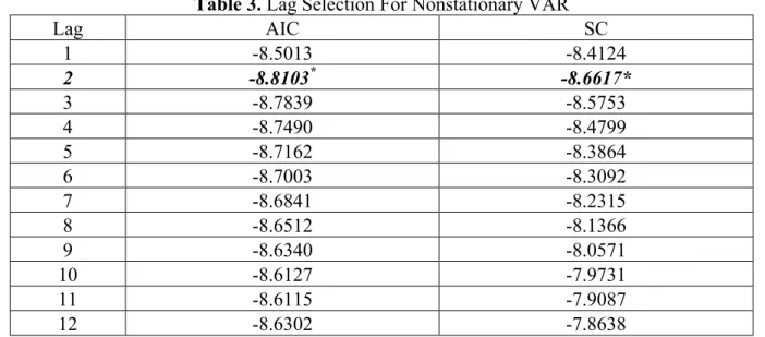
One of the important issues in VAR modelling in the context of forecasting literature is whether to transform the data into stationary form or to carry out the analysis in levels. In dealing with this issue, VAR forecasting is performed with both log-level (nonstationary) and first difference (stationary) series. AIC (Akaike Information Criterion) and SC (Schwarz Criterion) criteria are used to determine the order of VAR models. Optimal lag-length is acquired by testing down from a maximum 12-lag system until the minumum AIC and SC values are achieved. After applying this procedure, the appropriate lag is chosen as 2 for nonstationary (NSVAR) model. On the other hand, lag length for stationary VAR (SVAR) process is determined as 1. Table 2 and 3 show the results of the order selection procedure.

25

Table 3. Lag Selection For Nonstationary VAR

Lag AIC SC 1 -8.5013 -8.4124 2 -8.8103* -8.6617* 3 -8.7839 -8.5753 4 -8.7490 -8.4799 5 -8.7162 -8.3864 6 -8.7003 -8.3092 7 -8.6841 -8.2315 8 -8.6512 -8.1366 9 -8.6340 -8.0571 10 -8.6127 -7.9731 11 -8.6115 -7.9087 12 -8.6302 -7.8638 *Minumum Values

Table 4. Lag Selection For Stationary VAR

Lag AIC SC 1 -8.8052* -8.7161* 2 -8.7858 -8.6368 3 -8.7499 -8.5406 4 -8.7155 -8.4456 5 -8.7057 -8.3748 6 -8.6862 -8.2939 7 -8.6538 -8.1997 8 -8.6341 -8.1179 9 -8.6119 -8.0331 10 -8.6045 -7.9628 11 -8.6171 -7.9120 12 -8.6773 -7.9085 *Minumum Values

Therefore, the following dynamic simultaneous equations have been obtained for NSVAR model t i i i t i i t i t

c

LUSD

LTEFE

u

LTEFE

=

+

∑

+

∑

+

= = − − 2 1 2 1 0

α

β

(4.5) t i i i t i i t i t

c

LUSD

LTEFE

u

LUSD

=

+

∑

+

∑

+

= = − − 2 1 2 1 1

γ

θ

(4.6)

26 and SVAR model:

t t t t

a

DLUSD

DLTEFE

u

DLTEFE

=

₀

+

α

~

_{1 −1}

+

β

~

_{1 −1}

+

(4.7) t t t t

a

DLUSD

DLTEFE

u

DLUSD

=

₁

+

γ

~

_{1 −1}

+

θ

~

_{1 −1}

+

(4.8)

Both models are estimated by OLS and first equation of each model is used for out-of-sample forecasting.

4.2.3 Neural Network Models

Economic theory frequently suggests nonlinear relationships between variables and many economists believe that the economic relations are nonlinear. Thus, it is interesting to make forecasts by constructing the nonlinear relationship between variables examined in our study.

Two different ANN architectures are set up in an attempt to form a class of flexible nonlinear models. The architecture for the stationary series is denoted SANN and the second one designed for nonstationary series is named NSANN. Input layers are formed with respect to modelling methodology for VAR models. Moreover, our ANN models have the multivariate (vector) structure.

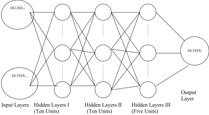
The following figures show the architectures of the ANN models used in our forecasting analysis. Note that forecasting with ANNs was performed by updating the sample period for each out-of-sample forecasts. Neural Network toolbox in MATLAB 6.0 software was used for the application.

27

Output Layer Hidden Layers I Hidden Layers II

(10 Units) ( 10 Units) Input Layers

Figure 9. Backpropagation Neural Network Architecture for Nonstationary Series

The architecture above has the following nonlinear specification:

)

)

(

(

)

(

10 1 10 1

∑

∑

= =

′

′

′

+

′

′

+

′

=

j j t t t t

X

G

X

F

G

X

LTEFE

λ

γ

λ

β

γ

λ

(4.10)

where

X

_t

=

LTEFE

_t−1

,

LTEFE

_t−2

,

LUSD

_t−1

,

LUSD

_t−2 is the input matrix. On the other hand, for the stationary neural network structure, the following relation is imposed:

∑

∑

∑

= = =

′

′

′

′

+

′

′

+

′

=

10 1 10 1 5 1

)

)

(

(

)

(

j j t j t t t

X

G

X

F

G

X

DLTEFE

λ

γ

λ

θ

β

γ

λ

(4.11)

where

X

_t

=

DLTEFE

_t−1

,

DLUSD

_t−1 is the input matrix. Note that these nonlinear ANN specifications imply that for the nonstationary ANN , there are two hidden layers, each consisting 10 neurons, while for stationary ANN there are three hidden layers, each with 10

LTEFEt-1

LTEFEt-2

LUSDt-1

LUSDt-2

28

neurons except the last one which has 5 neurons. Moreover, each hidden layer has sigmoid transformation function for both stationary and nonstationary ANNs.

Output Layer Input Layers Hidden Layers I Hidden Layers II Hidden Layers III

(Ten Units) (Ten Units)

(Five Units)

Figure 10. Backpropagation Neural Network Architecture for Stationary Series

4.2.4 The Exponential Trend Model (ETREND)

The other nonlinear model is chosen by considering the shape of the TEFE series in the level. It is seen that the series have the tendency to exponentially increase in time. Thus, we consider the following nonlinear model specification to generate the out of sample forecasts for the inflation variable.

t

t

T

TEFE

=

α

₁

exp(

α

₂

)

+

ε

(4.12)

where T is the time trend. Autocorrelation is removed with AR(2) transformation of the model which indicates the following specification :

DLUSDt-1

DLTEFEt-1

29

[

]

[

]

}

)

2

(

exp

{

}

)

1

(

exp

{

)

exp(

2 1 2 2 2 1 1 1 2 1

−

−

−

−

−

+

=

− −

T

TEFE

T

TEFE

T

TEFE

t t t

α

α

β

α

α

β

α

α

(4.13)

This equation is estimated by nonlinear least squares. MFIT 4.0 software package was used for the estimation. The following table shows the results.

Table 5. Estimation of ETREND Model

The coefficients given in Table 5 are used for the out-of-sample forecasts.

4.5 Forecasting Performance Evaluation

Out-of-sample forecast period starts at January 1999 and ends at June 2001. The sequential estimation strategy is employed to generate out-of-sample forecasts for one to four period horizons. All of the models examined in this study were reestimated at each forecast period after the forecast value for the latest month were added to the sample back.

Root Mean Square Error (RMSE) criterion is used to compare the models in terms of their forecast performances. The RMSE criterion is used because, as noted by Diebold and Lopez (1996), it continues to be the forecast accuracy criterion most commonly applied researchers.

Parameter Estimation Standard Error T-Ratio 1

α

12.64 0.0134 9.6743 2

α

0.0399 0.0039 10.0354 1

β

1.5893 0.0598 26.5461 2

β

-0.61175 0.06544 -9.3478 2

R

.99983 DW-statistic 1.9783 AIC -1278.8

30

Admittedly, however, as indicated by Clements and Hendry (1993), Armstrong and Fildes (1995), there are reasons that some researchers may generally prefer other forecast accuracy criteria. RMSE is computed for the forecasted value of the wholesale price index in the logarithmic difference form. Moreover, mean errors (MEs) are calculated for the out-of-sample forecasts and shown in Table 7 with the results of RMSE in Table 6.

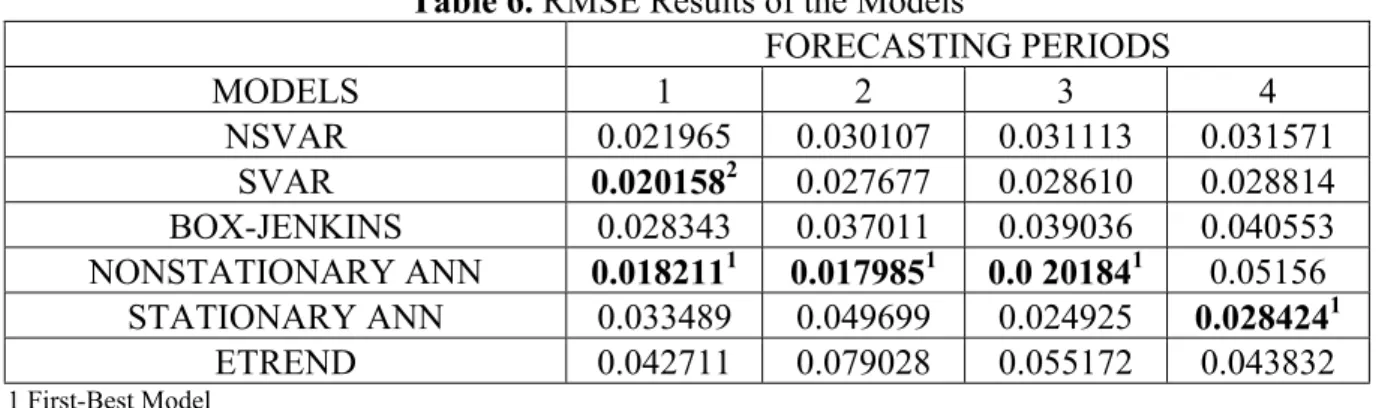
The inflation forecasts from the nonstationary ANN model were slightly better than the forecast values acquired from the others since one, two and three period ahead predictions are taken into account. On the other hand, the stationary ANN model outperforms in the four-step forecasts. The SVAR and NSVAR models give the similar forecast values, whereas Box-Jenkins and ETREND have the largest bias in inflation forecasting. Moreover, SVAR model outperforms the other models in both one and two-period ahead forecasts. On the other hand, stationary ANN is the second-best model for three-period ahead forecast. Table 7 shows that ME values of all the models except ETREND are positive, indicating that there are upward biases except in the case of ETREND which has a downward bias in one-period ahead forecasts. Moreover, three and four period ahead forecasts, all the models possess upward biases.

31

Table 6. RMSE Results of the Models

FORECASTING PERIODS MODELS 1 2 3 4 NSVAR 0.021965 0.030107 0.031113 0.031571 SVAR 0.0201582 0.027677 0.028610 0.028814 BOX-JENKINS 0.028343 0.037011 0.039036 0.040553 NONSTATIONARY ANN 0.0182111 0.0179851 0.0 201841 0.05156 STATIONARY ANN 0.033489 0.049699 0.024925 0.0284241 ETREND 0.042711 0.079028 0.055172 0.043832 1 First-Best Model 2 Second-Best Model

Table 7. ME Results for the Models

FORECASTING PERIODS MODELS 1 2 3 4 NSVAR 0.025498 0.058336 0.096748 0.137411 SVAR 0.032821 -0.000570 0.000692 0.000604 BOX-JENKINS 0.016284 0.044537 0.080042 0.119340 NONSTATIONARY ANN 0.033333 0.001038 0.000349 0.001775 STATIONARY ANN 0.008535 -0.003509 0.005081 0.001697 ETREND -0.000749 -0.010517 0.000956 0.008641

4.4 The Combination of Forecasts

It is observed that the nonstationary ANN, stationary ANN and SVAR are superior to other model forecasts in one-step prediction. It seems like we can improve our forecasts by combining forecast values from these three models.

We first consider the combination of forecasts using fixed weights:

t , 2 t , 1 1 t wf (1 w)f y ₊ = + − (4.14)

where f and _1,t f_2,tare one-step ahead unbiased forecasts of y_t+1 made at time t two using competing models. The choice of fixed weight (w) can be determined by reference to the minumum errrors which have zero mean and are uncorrelated. Thus, w is calculated from the ratio of the sums of squared errors:

32

(

)

(

)

(

)

∑

∑

∑

= = + + = +

−

+

−

−

=

_T t T t t t t t T t t t

f

y

f

y

f

y

w

1 1 2 , 2 1 2 , 1 1 1 2 , 2 1

~

~

~

ˆ

(4.15)

where

f

~

_1,tand

~

f

_2,t are in-sample forecast values.

Second, given a series of past outcomes and the alternative forecasts, Granger and Ramanathan (1984) propose determinig weights for the combination by linear regression of the outcomes on the forecasts. The following regression equation is implemented to allow the coefficients (weights) to vary as a function of forecast errors:

1 t t , 2 t 2 4 t , 1 t 1 3 t , 2 2 t , 1 1 1 t w f w f w f w f y ₊ = + + λ + λ +ε ₊ (4.16) where    − 〈 = λ + otherwise 0 0 f y if 1 t 1 1,t t 1 and    − 〈 = λ + otherwise 0 0 f y if 1 _{t 1 2,t} t 2

are the slope dummy variables reflecting the change in the slope of the regression equation.

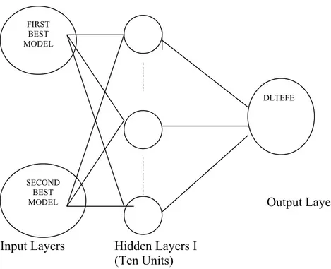
Third, a simple neural network model is introduced to make a forecast combination. This is similar to the fixed weight approach. However, the weight is obtained by the following ANN specification:

)

(

10 1 1

∑

= +

=

′

+

′

i i t

x

F

x

DLTEFE

λ

β

λ

(4.17)

where

x′

is the input vector referring to out-of-sample forecasts of NSANN, SVAR and NSVAR models.

DLTEFE

_t+1 is the actual values for the period between 1999.01 and 2001.06. The relevant architecture is given in the following figure.

33

Output Layer

Input Layers

Hidden Layers I (Ten Units)

Figure 11. Backpropagation Network for Forecast Combination

When combined forecasts are computed as described above, the resulting RMSEs for the out-of-sample period turn out to be as in Table 8.

Table 8. Forecasts for One-Period Ahead Forecasts

MODELS FIXED WEIGHT CHANGING WEIGHT ANN WEIGHT

NSANN and SVAR 0.019098* 0.015158 0.0006945

NSANN and NSVAR 0.021036 0.014734* 0.000396*

NSVAR and SVAR 0.021903 0.022389 0.0007123

*Minimum values

The results presented in Table 8 provide evidence that the regression approach with changing weights is relatively superior to the ratio approach with fixed weights for the combined

FIRST BEST MODEL SECOND BEST MODEL DLTEFE

34

forecasts. Furthermore, encouraging results are obtained by combining nonstationary ANN and the NSVAR, indicating that combining these models generates better forecast values than the other possible model combinations. Although combination of the nonstationary ANN model and the NSVAR forecasts based on the regression approach produce almost 19% reduction relative to the best single model (i.e., nonstationary ANN) forecasts, combination performed with ANN weights provides 98 % decline in out-of-sample RMSE.

35

CHAPTER 5

CONCLUSIONS

In this thesis, inflation forecast performances of alternative models were examined for Turkish economy. Despite a lack of theoretical studies, many researchers believe that forecasts obtained through nonlinear models are superior to those from linear models, when the underlying relationship between variables is nonlinear. For this reason, a variety of linear and nonlinear models was considered using stationary and nonstationary data in search of the best model in terms of the forecast performance.

Three types of time series were used by expressing values in levels, logarithmic levels and first differences. The series in logarithmic levels (nonstationary) and first logarithmic differences (stationary) were used in Box-Jenkins Model, NSVAR, SVAR, NSANN, and SANN models, whereas the series in levels was only used for ETREND. The use of different types of time series data allowed for observation of their effects on the forecasting performances of the models. It was observed, based on the results, that combination of models including nonstationary series improved inflation forecast performance in terms of the RMSE criterion.

Nonlinear neural network models considered in the thesis showed a generally better performance than the others. However, when the combination of forecasts from alternative models were considered, linear (NSVAR) and nonlinear (NSANN) model forecast combinations turned out to be more accurate than other combinations.

36

A simple combination technique to be performed with ANN was also proposed in the thesis, and it was shown that a considerable decline in RMSEs of the combined models could be achieved using this technique. Hence, it was argued that the proposed technique may be preferred to the well known techniques involving fixed and changing weigths.

It is concluded that the combination of NSANN and NSVAR forecasts based on regression approach and the ANN approach produce better out-of-sample forecasts than the other models.

37

BIBLIOGRAPHY

Adya, M.,and F. Collopy. 1998. “ How Effective are Neural Nertworks at Forecasting and Prediction ? A Review and Evaluation,” Journal of Forecasting 17:481-

495.

Armstrong, J.S., and F.R. Fildes. 1995. “ Correspondence on the Selection of Error Measures for Correspondence among Forecasting Methods,” Journal of Forecasting, 14: 67-71.

Campbell, J.Y., and P. Perron. 1991. “Pitfall and Oppurtunities:What Macroeconomist Should Know About Unit Roots,” In NBER Macroeconomics Annual,O.J. Blanchard and S. Fischer (eds), pp.144-201. Massachusetts: Cambridge Press.

Clements., M.P. and D.F. Hendry. 1993. “On the Limitations of Comparing Mean Square Forecast Errors,” Journal of Forecasting, 12:617-637.

Cybenko, G. 1989. “Approximation by Superposition of a Sigmoid Function,” Mathematical Control Systems Signals 2:303-314.

Ertuğrul A., and F. Selçuk 2001. “A Brief Account of Turkish Economy:1980-2000,” forthcoming in Russian and European Finance and Trade.

Foster,B., F.Collopy and L.Ungar.1992. “Neural Network Forecasting of Short, Noisy Time Series,” Computers and Chemical Engineering 16 (12):293-297.

Funanashi, K. 1989. “On the Approximate Realization of Continuous Mappings by Neural Networks,” Neural Networks 2:183-192.

38

Granger, C. W. and R. Ramanathan. 1984. “Improved Methods of Combining Forecasts,” Journal of Forecasting, 3: 197-204.

Gorr, W. 1994. “Research Perspective on Neural Networks,” International Journal of Forecasting 10:1-4.

Hamilton, J.D. 1994. Time Series Analysis. New Jersey: Princeton University Press.

Hill, T., L. Marquez, M. O’Connor and W. Remus.1994. “Artificial Neural Network Models for Forecasting and Decision Making,” International Journal of Forecasting 10:5-15.

...,1996. “Neural Network Models for Time Series Forecasts,” Management Science 42: 1082-1092.

Kang, S. 1991. “An Investigation of the Use of Feedforward Neural Networks for Forecasting,” PhD Dissertation, Kent State University.

Kohzadi, N., M. S. Boyd, B. Kermanshahi and I. Kaastra. 1996. “A Comparison of Artificial Neural Network and Time Series Models for Forecasting Commodity Prices,” Neurocomputing 10:169-181.

Lachtermacher, G. and J.D. Fuller. 1995. “ Backpropagation in Time Series Forecasting” Journal of Forecasting, 14: 381-393.

Lütkepohl, H. 1993. Introduction to Multiple Time Series Analysis. Berlin: Springer – Verlag.