Analyzing the effect of consumer returns in a multi-period inventory system

(1)

ANALYZING THE EFFECT OF CONSUMER RETURNS IN

A MULTI-PERIOD INVENTORY SYSTEM

A THESIS

SUBMITTED TO THE DEPARTMENT OF INDUSTRIAL ENGINEERING

AND THE GRADUATE SCHOOL OF ENGINEERING AND SCIENCE OF BILKENT UNIVERSITY

IN PARTIAL FULFILLMENT OF THE REQUIREMENTS FOR THE DEGREE OF

MASTER OF SCIENCE

by

İsmail Erikçi

(2)

ii

I certify that I have read this thesis and that in my opinion it is full adequate, in scope and in quality, as a dissertation for the degree of Master of Science.

___________________________________ Prof. Nesim K. Erkip (Advisor)

______________________________________ Asst. Prof. Alper Şen

______________________________________ Assoc. Prof. Osman Alp

Approved for the Graduate School of Engineering and Science

____________________________________ Prof. Levent Onural

(3)

iii

ABSTRACT

ANALYZING THE EFFECT OF CONSUMER RETURNS IN

A MULTI-PERIOD INVENTORY SYSTEM

İsmail Erikçi

M.S. in Industrial Engineering Supervisor: Prof. Dr. Nesim K. Erkip

July 2012

Return of a sold item by a customer becomes tremendously common situation in many industries. Increase in the amount of returned items promotes return information to be a critical factor for inventory control. Undoubtedly another critical parameter for an inventory system is the length of the review period. Effect of the review period or length of the time-bucket is amplified with returned items, because available return information at a decision point is related to the frequency of the review. In this study, we analyze the effects of these two parameters over a multi-period inventory system where the length of a time horizon is fixed. Dynamic programming approach is used to calculate the optimal inventory positions. In dynamic programming, it is assumed that a fixed proportion of sold items are returned. Computational results are obtained to compare the effects of return information under different return proportions and period lengths. These results are used to conduct various analyses to explore the level of the advantage gained by using return information.

Keywords: Consumer returns, dynamic programming, periodic review inventory system

(4)

iv

ÖZET

MÜŞTERİ İADELERİNİN ÇOK PERİYOTLU ENVANTER

SİSTEMLERİNDEKİ ETKİSİNİN ANALİZİ

İsmail Erikçi

Endüstri Mühendisliği, Yüksek Lisans Tez Yöneticisi: Prof. Dr. Nesim K. Erkip

Temmuz 2012

Bir çok endüstride satılan ürünün müşteri tarafından iade edilmesi sıkça rastlanan bir durum haline gelmiştir. İade edilen ürünlerin miktarındaki artış iade bilgisinin envanter kontolü için kullanılmasını önemli hale getirmiştir. Şüphesiz ki envanter sistemi için diğer bir kritik parametre gözden geçirme periyodunun uzunluğudur. Gözden geçirme noktaları arasındaki zaman azaldıkça iade bilgisinin daha sıklıkla kullanılması olanaklı hale gelmektedir. Bu çalışmada, ürün iadesi (ve bilgisinin) olması ve envanteri gözden geçirme sıklığının değişmesinin etkisi analiz edilmektedir. En iyi envanter pozisyonları dinamik programlama yaklaşımı kullanılarak hesaplanmıştır. Dinamik programlamada, satılan ürünün sabit bir oranının iade edildiği varsayılmıştır. İade bilgisinin farklı iade oranları ve period uzunlukları altındaki etkisinin karşılaştırılması için sayısal sonuçlar elde edilmiştir. Bu sonuçlar iade bilgisi kullanılarak elde edilen avantajın seviyesinin bulunması için yürütülen analizlerde kullanılmıştır.

Anahtar sözcükler: Müşteri iadeleri, dinamik programlama, periyodik envanter sistemi

(5)

v

ACKNOWLEDGEMENT

I would like to express my sincere gratitude to my advisor Prof. Nesim K. Erkip for his invaluable guidance, support, supervision and useful suggestion throughout this work. He has supervised me with everlasting patience and encouragement throughout this thesis. I consider myself lucky to have a chance to work with him.

I am also grateful to Asst. Prof. Dr. Alper Şen and Assoc. Prof. Dr. Osman Alp for accepting to read and review this thesis. Their comments and suggestions have been invaluable.

I also would like to express my deepest gratitude to my family for their eternal love, support and trust at all stages of my life and especially during my graduate study. Their love and support have been a strength to me in every part of my life.

I am indeed grateful to Hazal Yüksel for his morale support, patience, encouragement and endless love since I met her. Life and the graduate study would have not been bearable without her.

I would like to thank to my precious friends Murat Özcan and Fevzi Yılmaz for their great friendship, moral support and endless help during my graduate study. I am also thankful to Fatih Harmankaya, Onur Uzunlar, Burak Koç and Oğuzhan Efe Şakrak all friends I failed to mention here for their friendship and support.

Finally, I would like to acknowledge financial support of the Scientific and Technological Research Council of Turkey (Tübitak) and Bilkent University.

(6)

vi

(7)

vii

LIST OF FIGURES

Figure 2.1 Options for Handling Returns from Vlachos and Dekker (2003)... 7

Figure 2.2 The reparable item system that is defined in Cohenx et al (1980) ... 8

Figure 2.3 The recovery management environment that is defined in Inderfurth (1997) ... 9

Figure 2.4 The structure of the environment of our problem ... 10

Figure 3. 1 Length of Period = 4*Length of Time Bucket ... 13

Figure 3. 2 Length of Period = 2*Length of Time Bucket ... 13

Figure 3.3 Example graph of ... 15

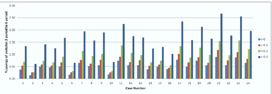
Figure 4.1Realistic savings of switching 3 period to 6 period in terms of percentage for all return proportions ... 32

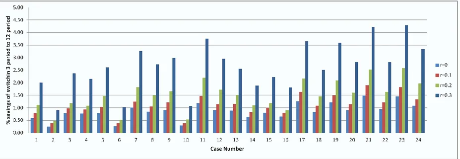
Figure 4.2 Realistic savings of switching 3 period to 12 period in terms of percentage for all return proportions ... 33

Figure 4.3 Advantage of operating with 6 periods instead of 3 period with c=120 instead of c=100, in terms of percentage ... 36

Figure 4.4 Advantage of operating with 12 periods instead of 3 period with c=120 instead of c=100, in terms of percentage ... 37

Figure B. 1 % realistic savings of switching 3 period to 6 period in terms of percentage for all return proportions for ... 81

Figure B. 2% realistic savings of switching 3 period to 12 period in terms of percentage for all return proportions for . ... 82

Figure B. 3 Advantage of operating with 6 periods instead of 3 period with c=120 instead of c=100, in terms of percentage ... 83

Figure B. 4 Advantage of operating with 12 periods instead of 3 period with c=120 instead of c=100, in terms of percentage ... 84

(9)

ix

LIST OF TABLES

Table 3. 1 Notation Table... 15

Table 4. 1 Average of % cost difference result of models that are developed in MATLAB and ARENA ... 24

Table 4. 2 Minimum of % cost difference result of models that are developed in MATLAB and ARENA ... 24

Table 4. 3 Maximum of % cost difference result of models that are developed in MATLAB and ARENA ... 24

Table 4. 4 Values of parameters that are used to generate different cases... 25

Table 4. 5 Summary of % savings of switching 3 review period to 6 review period or 12 period for all return proportions ... 31

Table 4.6 Summary of % realistic savings of switching 3 review period to 6 review period or 12 period for all return proportions ... 34

Table 4. 7 Extra advantage of shortening period length of items when purchased cost instead of , in terms of percentage ... 38

Table 4.8 Extra advantage of shortening period length of items when purchased cost instead o f , in terms of percentage ... 39

Table 4. 9 Summary of results for all period lengths and for all return proportions. 41 Table 4. 10 Summary of results without sunk cost for all period lengths and for all return proportions. ... 42

Table 4. 11 Summary of results % savings of switching from 3 review period with to 12 review period with various return proportions ... 44

Table 4. 12 Summary of results % realistic savings of switching from 3 review period with r=0 to 12 review period with various return proportions ... 45

Table 4.13 % loss of not operating optimally ... 48

Table 4. 14 % realistic loss of not operating optimally... 49

Table A. 1 Total Costs for 12 period problems when and ... 56

(10)

x

Table A. 13 Total Costs for 12 period problems when and per time bucket ... 68

(11)

xi

Table A. 23 Total Costs for 3 period problems when and per time bucket ... 78 Table A. 24 Total Costs for 3 period problems when and per time bucket ... 79

(12)

1

Chapter 1

Introduction

Over the last decades, consumer return policies have become one of the vital fields in industry, especially in apparel and electronics. The value of returned products exceeds $100 billion each year in U.S and $13.8 billion are spent in electronic industry to rebox and resell returned products. (Stock, 2002 and Lawton, 2008). Even though the products are not defective, consumers have a tendency to return the products. Only 5% of returns are truly defective (Lawton 2008). The proportion of returns can be ranged from 11% to 20% in electronics and up to 35% in the apparel industry (Guide 2006). Internet sales and rapid progresses in technology are the main triggers of consumer returns. In other words, higher anticipation from product features and lack of understanding of the product by consumer lead to increase in product returns. Some companies have enhanced new strategies to cut down the

(13)

2

returns such as TV makers who put extra notices and the computer companies engrave customers’ name on a computer.

Some extra risks arise for consumers due to the advances in high-level technological products and remote purchases. The leniency of return policy is one way of minimizing the inherent consumer risk. Companies are commonly adapted to “no question asked” 100% money-back guarantees to create their competitive advantage because return polices has profound effects on consumer demand, and consumers’ buying behavior. Around 90% of consumers highlight that return policies become much more crucial while buying new or unknown product by online or by catalog retailer. Moreover, consumers have a tendency not to shop from a retailer, if the retailer’s return policy is inconvenient (Market Wire 2007). Even if return policies affect consumer demand in a positive manner, there is also a side effect of lenient return policies. Firstly, lenient return policies are costly to operate because of stocking, refurbishing or reboxing of returned items. Secondly, lenient return policies give consumer an opportunity to abuse the policy such as borrowing an item for special purposes. Some of the known examples that can be named as an abuse are returning TV sets after Super Bowl or return of camcorders after a wedding (Wood 2001).

The positive and negative impacts on return policies make managers found themselves in dilemma. That is, different return policies are introduced by different managers for the same type of product (Davis et al. 1998). Another study shows that permissible period for returned items fluctuate as well, in a large interval (Stiner 2004). There are mainly 4 parameters which differentiate return policies from each other, these are:

1. Return price 2. Return period

3. Assumption about return decision of customer 4. Options for handling of return

(14)

3

In this study, we consider that the retailer operates in an environment as if the time frame was multi-period and there was a lead-time between the retailer and supplier. It is assumed that the retailer adapts no return policy in a base case, and in alternative cases the retailer adapts a return policy that gives full refund for the returned items. Basically, there is no fixed ordering cost; but there are salvage, backorder, holding and penalty costs. Therefore, in a base case it is backordered multi-period Newsboy problem with lead-time. In alternative cases, predetermined proportions of sold items are returned by the customer who gets a full refund. Returned items can be sold in the next period. There is no remanufacturing or restocking cost for returned item. Therefore, the alternative cases can be called as multi-period backordered Newsboy problem with returns and lead-time.

This study tries to identify the benefit of using information of returns by looking at the inventory system more frequently. To make this identification, we have fixed the length of time horizon but change the period length while the length of lead-time is constant. By this approach, the benefit of looking at the inventory system more frequently and use of return information can be identified. Comparisons among base case and alternative cases provide managerial insights for setting return policy and reviewing frequency as well.

In classical periodic inventory systems, period length is not considered as a decision variable. Commonly in the literature, period length is assumed to be fixed and the analysis is made over cost parameters. However, in a finite time horizon period length has a profound effect over the system because the period length is a parameter for deciding the review frequency of inventory. Treating period length as a decision variable provides a chance to analyze the effect of the period length over total costs, optimal inventory levels etc. To analyze this effect, we define base time unit called time bucket. Length of time horizon and period lengths are defined in terms of time bucket. In this study, we investigate the effect of period length over system by changing the number of time buckets in the period.

(15)

4

In this study, the problem that is briefly mentioned above is solved by dynamic programming. Base case formulation is quite similar to Porteus’ formulation and alternative cases are derived from the base case. In the rest of this study, when Porteus work is mentioned, we are referring to Porteus’ book chapter 4.2 that was published in 2002.

The rest of this thesis is organized as follows. In Chapter 2, the related literature is reviewed. In Chapter 3, the detail problem definition is given and the mathematical model is presented. The computational results are given and the comparisons are summarized in Chapter 4. The conclusion and possible further research areas can be found in Chapter 5.

(16)

5

Chapter 2

Literature Review

In this study, we consider finite periodic review inventory system with stochastic demand, deterministic lead-times for orders and consumer returns. We utilize dynamic programming approach to solve the problem.

Utilization of dynamic programming approach in the inventory management literature dates back to 1960s. Karlin (1960) formulates dynamic inventory model where demand distribution can vary from period to period. He derives optimal policy for both convex purchase and linear purchase cost and there is a delivery lead-time. Veinott (1965) considers multi-product, dynamic non-stationary inventory problem. Under special conditions, he derives a policy for minimizing the expected discount cost over infinite time horizon. Kaplan (1970) considers dynamic inventory problem with stochastic lead-time where there is a fixed setup, linear order, convex holding and shortage cost. Porteus (2002) shows that base stock policy is optimal for each period of finite-horizon problem assuming that the terminal value function is convex.

(17)

6

Heyman (1978), Simpson (1978), Cohen (1980) and Inderfurth (1997) utilize dynamic programming approach in their model where they consider returns.

There is considerable research on stochastic inventory models with product returns. Simpson (1978) considers a finite periodic review inventory system where supplies and returns are instantaneous. The other assumption of his study is that demand and return streams are joint random variables. The lead-time for returned item is fixed whereas it is zero for the orders. Kelle and Silver (1989) study on the model where fixed proportion of satisfied demand is returned and fixed proportion of returned items can be used. They also regard fixed order cost and stochastic sojourn time of returned item. Muckstadt and Isaac (1981) model the problem by considering single item, multi-echelon environment using continuous review policy. They assume that demands and returns are independent streams, returned and serviceable items are only at retailer level. They assume that system return rate is less than system demand rate. Yuan and Cheung (1998) model the problem for similar environment with an (s,S) order policy via Markovian formulation. Their policy is based on the number of items on-hand and the number of items that are sold in the market. In their model, return stream depend on demand stream. They consider Poisson demand and exponentially distributed market sojourn time. Fleischmann et al (2002) derive optimal control policy for infinite horizon system where the order cost and procurement lead-time are fixed; streams for demand and return are independent. Another branch of research examines single period problem by considering consumer returns. Vlachos and Dekker (2003) elaborate on various return handling options. They investigate an environment such that order decision is made before the beginning of the selling period and returns can be used to satisfy new orders. They list return handling options as in Figure 2.1 and they derive optimal order quantity for each option.

(18)

7

Figure 2.1 Options for Handling Returns from Vlachos and Dekker (2003) Mostard et al (2005) investigate catalogue/internet case where returned item can be resold if there is a sufficient demand. They assume that order is given before the selling season. What makes the study different than previous studies in the literature is the assumption of unknown distribution for demand. They derive expression for the order quantity which is the obtained distribution-free setting. Mostard and Teunter (2006) consider that a product cannot be resold twice because returned products are generally sold at the end of season. Therefore, there is not enough time to return the sold product. Under this assumption, optimal order quantity is higher than the order quantity where returned item can be resold more than once. Ketzenberg and Zuidwijk (2009) divide one selling season into two periods to formulate the case where returns at the first period can be resold at the second period but returns at the second period may only be salvaged. They also consider return policy and price effects over the demand in their model. They derive optimal decision strategy for deterministic model but in the stochastic model they perform the experimental design.

Davis et al (1995) present a model which assumes that the consumer can only evaluate product after purchase. The model formulates consumer valuation as a Bernoulli random variable in which the product may either match consumer needs or may not. Che (1996) does not restrict consumer valuation with any distribution but consider risk aversion. Su (2009) consider the case where the customer realizes his valuation over the product only after the purchase. They investigate impacts of full

No fixed Cost No fixed Cost

Fixed Cost Fixed Cost

Returns

Secondary Market Reuse

(19)

8

return policies and partial return policies. They propose contracts to coordinate supply chain with consumer returns.

Cohen et al (1980) assume that a fixed proportion of satisfied demand is returned and only fixed proportion of these returned items can be added to the serviceable inventory. Presentation of this environment is given in Figure 2.2. In our model, we consider a similar environment but we assume that all returned item can be resold whereas in their model some fraction of returned items can leave the system forever. They consider zero lead-time for orders while our model considers fixed lead-time for orders.

Figure2.2 The reparable item system that is defined in Cohen et al (1980) Inderfurth (1997) addresses the environment such that there is finite periodic review system with stochastic demand and stochastic returns. In his model, demand stream and returns streams are independent from each other. He also assumes that disposal of returned item inventory is available at each period. He considers that the supplies and returns have lead-time greater than zero but they are not necessarily equal. Represantation of his environment is given in Figure 2,3. In our study, we disregard

Fraction of items are condemned and leave the system

External Repair Facility

External Demand Issue Stock

External Supplier

Fraction of items are repaired and returned some fixed periods

later

Items may be ordered from external supplier with zero

lead-time Failed units are shipped

immediately to repair facility

Stock is issued to replace failed units

(20)

9

disposal of returned item inventory, except in the terminal period left over inventory may be salvaged. The other difference of our study from Inderfurt (1997) is we assume fixed proportion of sold products return after fixed market time.

Figure 2.3 The recovery management environment that is defined in Inderfurth (1997)

This study deals with single product inventory system over finite time horizon where orders have fixed lead-time and fixed proportion of sold products return after fixed market time. The representation of our model is given in Figure 4.3. We assume that there is no fixed setup cost, but there is a linear purchase cost, convex holding and shortage cost. We disregard disposal of inventory by assuming that the leftover inventory on hand of previous period can never be greater than the optimal level of current period. Another assumption we make is that all returned items can be used to satisfy demand. We investigate a reduction in the total cost while increasing the frequency of inventory review. Increasing the frequency of inventory review means, shortening period lengths while length of a time horizon is fixed. As we mentioned in the previous chapter, by treating period length as a decision variable we analyze the effect of period length over the inventory system. Different values of period length affect available information about inventory system status. Hence by changing period lengths, we also try to elaborate on the benefit that can be gained by using information of returned item. This type of analysis has not been addressed in the literature before. remanufacturing (r) disposal (d) procurement (p) returns Ŕ Inventory of serviceables Inventory of returned products lead-time:λr lead-time:λp

(21)

10

Figure 2.4 The structure of the environment of our problem

probability 1-p

Accepted by customer lead-time-λs demand

Supplier _supplies Retailer Customer

probability p Decided to return lead-time-λr

(22)

11

Chapter 3

Problem Definition and Mathematical

Model

In this chapter, we elaborate on environmental assumptions, model formulation and lastly properties of the model.

3.1. Environmental Assumptions

We define time buckets as a smallest time unit in our setting. Each parameter in the model such as holding cost, shortage cost, discount rate is defined for a time bucket (unit time). Length of period, time horizon, order and return lead-times are also defined in terms of time buckets. The aim of using time buckets is preserving consistency between problems as much as possible. Time buckets is the mechanism that provide consistency in cost calculation of different setting of problem.

(23)

12

Time horizon consists of periods and periods consist of time buckets. The length of a time bucket is fixed and also the length of a time horizon is fixed, hence the number of time buckets in the time horizon is fixed. A time bucket cannot be divided into any smaller part; that is, period length is a multiple of a time bucket. The number of period in the time horizon is adjusted with period lengths. Let time horizon be equal to time-buckets, and let the length of a period be defined as time-buckets, hence we have period problem setting. In this example, let holding and shortage costs for time buckets be and respectively; discount rate is , then for a period consisting of time bucket holding and shortage costs are and , discount rate for a period is equal to .

We assume that order lead-time is fixed and independent from period length. Let order lead-time be equal to time buckets and period length be equal to time buckets then order-lead time is equal to 2 periods. In another setting if period length was equal to time buckets then order time is equal to 4 periods. Return lead-time totally depends on the period length. Since a sold item can be added to the inventory only at the beginning of the next period therefore, return lead-time is equal to period length.

We assume order of events in any period is determined as follows. Firstly, items returned from previous period are added to inventory, secondly, if order is given then the order given a lead-time ago is received. Afterwards demand for this period occurs and items are sold. Lastly, cost is evaluated. Figure 3.1 (3.2) represent example of a setting where length of time horizon is 12 time buckets and period lengths is 4 (2) time buckets. Length of lead-time is 1 (2) period at Figure 3.1 (3.2).

(24)

13

Figure 3. 1 Length of Period = 4*Length of Time Bucket

Figure 3. 2 Length of Period = 2*Length of Time Bucket

In the literature, there are some methods that we mentioned in Chapter 2 on how to make consumer return decision, such as using probability function dependent or independent from demand, valuation functions, proportion of sales etc. We use fixed proportion of expected demand as returned assumption but there is a critical point to emphasize; if we disregard this assumption then Markovian property cannot be preserved when an order lead-time is greater than one period. Because in the case where order lead-time is greater than one period, amount of sales and amount of returned items during lead-time depends on past decisions. Therefore, when order lead-time is greater than one period, the decision maker can act optimally only if he/she knows the previous decisions. Because the amount of returned items depends on past decisions, Markovian property cannot be preserved. To overcome this challenge we assume that the amount of returned item is a fixed proportion of expected demand. Hence, the amount of returned items is known for the next periods and independent from past decisions then Markovian property is preserve.

(25)

14

We assume that remanufacturing cost and remanufacturing time for returned items are negligible. There is no difference between returned items and ordered items in a sense that both can be used to satisfy demand. After an item is sold, the beginning of the next period is the only available point for a customer to return this item. If a customer does not return the item at that point, it can be assumed that the customer keeps the item. Since time horizon is finite, there is a special case at the last period for returned items. That is, at the end of last period whether excess inventory is salvaged or backlogged demand is satisfied with paying extra penalty cost in case of shortage. Cost evaluation is made and time horizon is ended. Proportion of sold items at the last period is returned after time horizon ended; however, because they cannot be salvaged or cannot be used to satisfy backlogged demand, they are disregarded. It can be interpreted as if items that are sold at the last period could not be returned.

3.2. Model Formulation

In this section we construct a model by considering environment that is defined above. We use notation in Table 3.1.

Notation Definition

Unit purchasing cost

Unit penalty cost of backlogged demand Unit holding cost of leftover inventory

Unit salvage value for leftover inventory at the end of time horizon

Unit penalty cost of unsatisfied demand at the end of time horizon

Order lead-time in terms of period

Return proportion

Mean demand

(26)

15

Discount rate

Table 3. 1 Notation Table

We use backward dynamic programming approach to model the problem. Let inventory at the end of the last period N be x, then terminal cost is where

is a convex function when . There is a graph of in Figure 3.3 when and .

Figure 3.3 Example graph of

Holding and shortage cost for periods is a bit different than Porteus’ case in terms of returned items and lead-time. Let consider order is given and inventory position is increased to y, then expected holding and shortage cost L(y) is incurred.

is demand that occurs during lead-time and is demand during one period. The first term in is expected holding cost and second term is expected shortage cost. is the inventory position after order is given. Order can be added to inventory

(27)

16

after periods. Hence, effect of order can be seen period later. In the cost calculation, period demand is subtracted from inventory position and items that are returned during lead-time is added. We make important assumption about the amount of returned item that we mentioned in the previous section. Number of returned items is proportion of sales and sales depend on demand and inventory on hand. Therefore orders that are given before period t are also critical because they have impact on inventory on hand. Impact of order decision at period t depends on past decisions therefore, Markovian property cannot be preserved. We assume demand is fully satisfied in the past and fixed proportion of demand is returned. Instead of sales, we use demand to calculate returns therefore, we can make decisions independent from past decisions. Hence, is not a function of sales but a function of demand.

Now, we can write the optimality equations for this environment for 1< t < N-1 where N is the number of periods:

x is a state in period t before giving an order, y is an inventory position after giving an order. is order cost, is expected holding and shortage cost and is expected present value of future cost such that starting at period t+1 in a state and acting optimally for the rest of the time horizon. is the inventory position and is the current period demand so it is subtracted from . To decide the next period starting state, the returns that are related to sales of current period should be added to Amount of returned items is calculated with .The term can be

(28)

17

interpreted as the expected inventory on hand at the beginning of the period. Then the term can be interpreted as expected return. When we use following equation,

For period ,

for each x. (3.5)

We can rewrite optimality equations as

(3.6)

where

(3.7)

(3.8)

We construct the model using backward dynamic programming approach; we elaborate on the properties of model in the next section.

3.3. Properties of the Model

Porteus’ model is a special case of our model. If the following parameter set is chosen then our model can be reduced to Porteus’ model.

(3.9)

Using this parameter set we can rewrite equations such as;

(29)

18 (3.11) (3.12) When we convolve and , can be re-written as follows;

(3.13) The structure that is defined by Porteus and our structure become the same. From this point, by following the same steps of Porteus starting from Lemma 4.3, the same results can be reached.

For other parameter sets, we use the same approach as Porteus did in Lemma 4.3 and Theorem 4.2 to show convexity of and optimality of base stock policy in each period of finite-horizon problem.

Lemma 1. If is convex, then following hold, a) is convex

b) is convex. Proof:

a) To prove that is convex, let firstly examine whether is convex or not. can be re-written as follows;

(30)

19 (3.14) where is (3.15) Since convexity is preserved under integration, proving the convexity of is sufficient. First derivative of is equal to

(3.16) where is cumulative density function of . is monotonically non-decreasing so is a convex function, hence is a convex function.

To sum up, proving the convexity of is sufficient to show that is a convex function because all other terms are convex.

b) Since convexity preserve under minimization and is a convex function

hence, is convex.

Theorem 1. A base stock policy is optimal in each period of a finite-horizon

problem.

Proof: By assumption, the terminal cost function is convex. Then, by Lemma 1 is convex hence is convex. Therefore, base stock policy is optimal for period N. For other periods it can be shown that is convex by iterating backward through the periods in the sequence t=N,N-1,….1.

(31)

20

In this chapter, first, the assumptions that are made about the problem environment are explained. We begin to construct our model by defining terminal cost function . In equation 3.2, the expected holding and shortage cost is defined. By the help of these two functions, optimality equations are derived. The boundary conditions are given in equation 3.4 and 3.5. The equations are re-written in 3.6, 3.7 and 3.8 in a way that they provide the setup for Lemma1 and Theorem 1. In section 3.3, it is shown that under specific conditions Porteus’ problem environment and our problem environment are equivalent. By using equations 3.10, 3.12 and 3.13, the optimality of base stock policy can be proven like in Porteus’ Theorem 4.2. In Theorem 4.2 Porteus proves that base stock policy is optimal in each period for finite horizon problem. In Lemma 1 and Theorem 1, we follow the steps of Porteus’ except we consider more general case. In Lemma 1, to show convexity of , since convexity of purchasing cost and convexity of expected future cost are trivial, we need to show that is a convex function. Using equations 3.14, 3.15 and 3.16, it is shown that is convex therefore is convex. Theorem 1 shows that base stock policy is optimal in each period for finite horizon problem using Lemma 1 and by iterating backward through the periods.

(32)

21

Chapter 4

Computational Results and

Comparison

In this section, we elaborate on the verification steps and analyze results of the model for varying value of parameters. We mainly analyze the effects of return proportion and length of period over total cost.

4.1. Verification of Computer Program

To explain the assumptions that were used during coding level, the results of the models that were developed in MATLAB and ARENA were compared and comparing MATLAB results with Porteus’ result are steps of our verification method.

(33)

22

4.1.1 Assumptions

In this section, we explain the assumptions that were made during the implementation phase. We implemented our model by using MATLAB. The code of the model can be found in Appendix E. To verify our model, we use Porteus’ results and we developed another model by using ARENA. The details of the verification are explained in the next sections.

We first assume that demand, the amount of returned items and inventory position are all discrete. This assumption is made because in a coding stage, we use matrix for demand, amount of returned items and inventory position where we need to define a base unit to assign matrix indices. Hence we decided to round decimal points and assume that demand, amount of returned items and inventory position are all integers.

The second assumption is made on the number of returned items. In the previous sections, we mention that a fixed proportion of demand is returned. By multiplying the satisfied demand with that proportion, the results are likely to be decimal numbers. We use this number to decide the next period state and inventory position that is not allowed to be decimal, therefore we need to round up the amount of returned items. Rounding is performed in a way that the amount of returned items is rounded up to the nearest integer.

The last assumption is made for demand and inventory position for first (lead-time) periods. We assume that the demand that occurs during the first period is equal to the inventory on hand. Demand is fully satisfied for the first periods and there is no excess inventory. This assumption was made because of the following reason; in ARENA, it is possible to have a simulation environment that uses sales to calculate the amount of returned items. However in MATLAB, we use demand to calculate the amount of returned items to preserve the Markovian property. Let us consider the following scenario; lead-time is four periods and starting inventory position is zero. Order is given and then demand occurs but demand is backlogged to

(34)

23

satisfy later periods because the inventory on hand is zero. According to model that is implemented in ARENA, there is no return for second, third and fourth period because the first order would come in fifth period. Since all the backlogged demand is satisfied at the beginning of the fifth period, it means there is an extreme sale in the fifth period and it will cause an extreme amount of returned item for the next period. In model that is implemented in MATLAB, the return flow is smoother because demand is used to calculate the amount of returned item. By assuming demand that occurs during the first period is equal to the inventory on hand, we can guarantee that we also have a smooth return flow in the ARENA model.

4.1.2 Comparison of MATLAB results and ARENA results

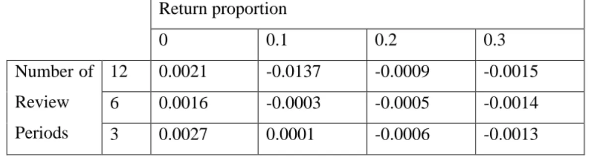
To verify the fact that the solution found by preserving the Markovian property is not significantly different from the solution without preserving the Markovian assumption, an ARENA model that could simulate the problem environment was built. The ARENA model uses inventory level as an input in addition to the inputs used in MATLAB model. Basically, there are two differences between the ARENA model and MATLAB model. The first difference is that, in MATLAB we calculate the optimal order up to levels by dynamic programming approach whereas in ARENA we simulate the problem environment with specific order up to levels that are already found in MATLAB model. The second difference is that, the ARENA model calculates the amount of returned items based on sales of the previous period whereas in MATLAB the amount of returned items are calculated based on expected demand. The view of interfaces of the ARENA model is found in Appendix C and the codes are in appendix D. Since we are planning to analyze the results based on the return proportion and review frequency the table of results is divided into 12 parts. For each cell of Table 4.1, we have 72 results that are calculated in MATLAB. We pick 10 out of these 72 cases for each cell and run the ARENA model for cases individually. Hence we get the results of the ARENA model for 120 different cases. Average, minimum and maximum differences are calculated for these 10 different cases. The results can be seen in Tables 4.1, 4.2, 4.3 in terms of percentages.

(35)

24 Return proportion 0 0.1 0.2 0.3 Number of Review Periods 12 0.0021 -0.0137 -0.0009 -0.0015 6 0.0016 -0.0003 -0.0005 -0.0014 3 0.0027 0.0001 -0.0006 -0.0013

Table 4. 1 Average of % cost difference result of models that are developed in MATLAB and ARENA

Return proportion 0 0.1 0.2 0.3 Number of Review Periods 12 0 -0.0152 -0.0027 -0.0033 6 0.0009 -0.0007 -0.0028 -0.0046 3 0.0007 -0.0006 -0.0022 -0.0039

Table 4. 2 Minimum of % cost difference result of models that are developed in MATLAB and ARENA

Return proportion 0 0.1 0.2 0.3 Number of Review Periods 12 0.0032 -0.0130 0.0004 0.0006 6 0.0028 0.0006 0.0048 0.0017 3 0.0062 0.0009 0.0011 0.0009

Table 4. 3 Maximum of % cost difference result of models that are developed in MATLAB and ARENA

As it can be seen from the tables above, the difference between the two models is insignificant. The results support the assumption which was made earlier to preserve the Markovian property does not always yield any significant difference in cost calculation. However the assumption provides us the chance of utilizing dynamic programming approach with less number of states.

(36)

25

4.1.3 Verification of MATLAB results by Porteus’ results

As a second method for verification, we use theorem 4.3 that Porteus states. The Porteus’ model and our model is equivalent when we set and . Theorem 4.3 states that the optimal order up to the levels for inventory positions are equal for every period in the specified environment. Let order up to levels be equal to where satisfies;

represents the cumulative distribution function of demand. In the table of results, there are 36 cases that are equivalent to Porteus’ problem environment. The results of all of these cases satisfy Porteus’ Theorem 4.3. Hence, it can be said that our model was correctly built and implemented.

4.2. Results

In this section we present results that are calculated in MATLAB. We calculate optimal order up to levels according to the values of parameters that are given in Table 4.4. Parameters Values 100, 120 5, 10, 15 1, 5 80, 100 100, 120 0.99, 1 0, 0.1, 0.2, 0.3

Table 4. 4 Values of parameters that are used to generate different cases These values are considered for one time-bucket. They are recalculated with respect to period length in Appendix A. Let period length be equal to 4 time-buckets then

(37)

26

with respect to period length. Parameters do not vary with respect to period length.

We consider a time-horizon with a length of 12 time-buckets. A review period can consist of 1, 2 or 4 time-buckets. In other words, we consider 12, 6 or 3 period problem respectively.

The demand for a time bucket is discretizing from normal distribution with mean 20 and standard deviation 2. The probability distribution of a demand for a period is calculated using determined distribution of time bucket. For instance, if a period consist of 4 time bucket then demand for this period has a probability distribution with mean 40 and standard deviation 4.

As we explained in the previous section in first periods, there is an enough inventory to satisfy demand and also there is no excess inventory for first periods. Let us consider a 12 period problem where a period length is equal to a time bucket length. Let be equal to 0.2. Inventory on hand for the first period is equal to mean of demand which is 20, and 16 for other periods. Demand that occurs for first periods is 20 for each period. Therefore the first period sales is equal to demand and it is 20 and that means 4 items will be returned and can be resold at the second period. Inventory on hand in the second period is increased from 16 to 20. This procedure continues in the same manner until the first order arrives. After first order arrives, demand is random variable with mean 20 and standard deviation 2. 6 period and 3 period problems also have the similar scenarios. The results that are taken from MATLAB runs can be seen in Appendix A.

4.3. Discussion of Results

In this section, we interpret the results of the model for varying values of the parameters, review frequency and return proportion. We conduct a set of analysis to explore the relations between cost, review frequency and return proportion. In the

(38)

27

analyses, comparisons are made over expected total cost. Expected total costs are calculated according to optimality equations that are defined in Chapter 3.

Since the unsatisfied demand is backordered to satisfy next period, at the end of time horizon all the demand is satisfied. This situation is valid for all cases independent from period length and return proportion. Hence the total cost includes a part that inevitably occurs because of cost of purchasing product to satisfy demand. This cost was treated as sunk cost and the analyses are conducted second time by disregarding sunk cost. Purchasing time can vary with period length, therefore holding and shortage cost is a function of review frequency. Disregarding sunk cost enables us to identify the relation between review frequencies and return proportion with remaining costs more clearly. The sunk cost can take different values in order to return proportion and discount rate. The discounted sunk cost can be calculated but using formula 4.1. In the analyses we disregard the minimum value of the sunk cost which is calculated according to formula 4.1. Sunk cost takes its minimum value when

where Firstly, we analyze the effect of frequency of review over total cost for each return proportion. We compare the cost of two cases where they only differentiate from each other by the frequency of review. The details of analysis can be found in 4.3.1. Secondly, we investigate the relation between purchase cost and advantage of high review frequency. Two cases are chosen and the only difference between them is the purchase cost and the costs of these two cases are calculated for different period lengths. We compare costs and try to identify which purchase costs are more advantageous in terms of cost under what conditions. The details of the analysis can be found in 4.3.2.

(39)

28

Lastly, the advantage of switching return proportion from zero to other values is analyzed. In this analysis, cases where there are no returned items are taken as base cases. We investigate in which period length is more advantageous to switching no return case to return cases. We repeat this analysis for each return probability. Details and figures can be found in section 4.3.3

The figures and tables in section 4.3.1, 4.3.2 and 4.3.3 belongs to cases where . Figures and tables for cases can be found in Appendix B.

As a notification, we use “realistic saving” as a term in the analyses where sunk cost is disregarded. When total cost that contains sunk cost is compared we use “saving” only.

4.3.1 Analysis of savings of switching between period lengths for each return proportion

The first analysis is conducted to identify the relation between period length and cost. We observe a change in cost in terms of percentage for each case. In other words, we investigate the percentage of savings of switching from one period length to another. The formula that is used to calculate this percentage can be written as follows;

Let us consider case number 1 in Table A.10 as an example where the number of review periods is 3 and the total cost is 14515. Now consider case number 1 in Table A.6 where the number of review period is 6 and the total cost is 14480. These two cases have same parameters but only differ from each other by period length. Then

(40)

29

savings of switching 3 review period problem to 6 review period problem for case 1 when is

The percentages for switching from 3 review periods to 6 review periods and 3 review periods to 12 review periods are calculated. The summary of results can be found in Table 4.5.

Let first focus on cases where ; the reason of saving is controlling inventory position and increasing frequency of orders. Since there is no return for these cases, cost advantage comes solely from frequency of controlling inventory position. When is not equal to zero there is a chance to use return information in decision points. As a verification of this claim, from Table 4.5, it can be seen that for all return proportion the average saving is higher than no return situation.

Same analysis is conducted with cost such that sunk cost is disregarded. In this case the effect of switching between numbers of period can be explored more explicitly. Formula 4.2 is modified in a way that sunk cost is disregarded.

By disregarding sunk cost we extract the inevitable cost from total cost. Hence we focus on the cost that can be influenced by change in number of period. Summary of results can be found in Table 4.6.

In both analyses, the percentage of saving is largest for all cases when for both switching from 3 review periods to 6 review periods and 3 review periods to 12

(41)

30

review periods. From Figure 4.1 and 4.2, it can be concluded that the magnitude of the percentage of realistic savings increases with return proportion.

(42)

31

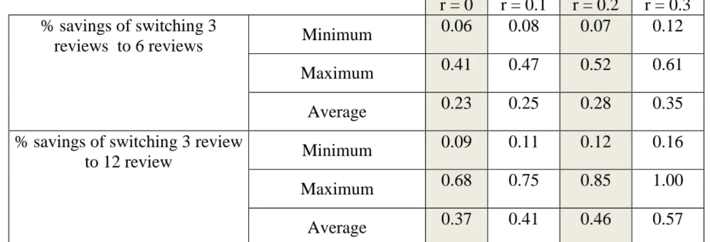
r = 0 r = 0.1 r = 0.2 r = 0.3 % savings of switching 3

reviews to 6 reviews Minimum

0.06 0.08 0.07 0.12

Maximum 0.41 0.47 0.52 0.61

Average 0.23 0.25 0.28 0.35

% savings of switching 3 review

to 12 review Minimum

0.09 0.11 0.12 0.16

Maximum 0.68 0.75 0.85 1.00

Average 0.37 0.41 0.46 0.57

(43)

32

(44)

33

(45)

34

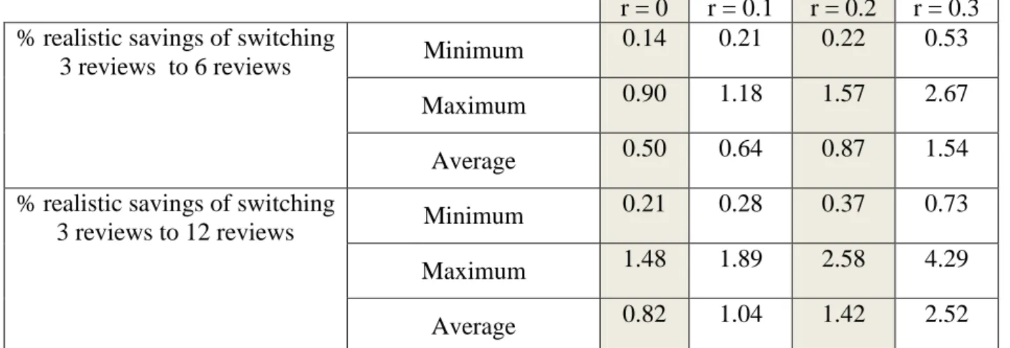
r = 0 r = 0.1 r = 0.2 r = 0.3 % realistic savings of switching

3 reviews to 6 reviews Minimum

0.14 0.21 0.22 0.53

Maximum 0.90 1.18 1.57 2.67

Average 0.50 0.64 0.87 1.54

% realistic savings of switching

3 reviews to 12 reviews Minimum

0.21 0.28 0.37 0.73

Maximum 1.48 1.89 2.58 4.29

Average 0.82 1.04 1.42 2.52

(46)

35

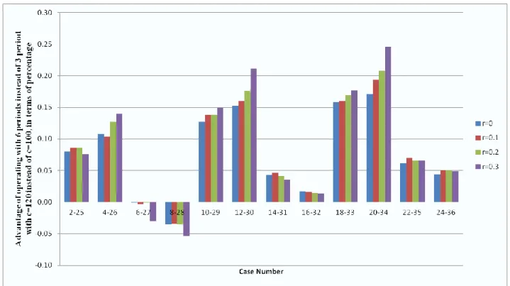
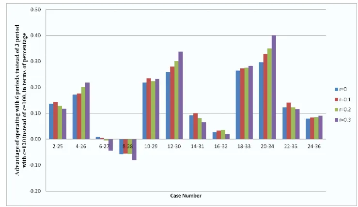
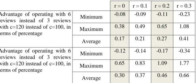
4.3.2 Analysis of the advantage of operating inventory system with more review periods for various unit cost items

In this analysis, we try to explore whether operating with more review periods with consumer returns in a fixed time horizon is advantageous for units with a high unit purchase cost or units with low unit purchase cost. This advantage is defined with following formula;

Let us consider Case 2 in Table A.11, we formulate a way to calculate the percentage of savings of switching from 3 review period to 6 review period in the previous section, formula 4.2. We calculate the same percentage for Case 25 in Table A.11. These two cases have the same parameter sets except they differentiate from each other by unit purchase cost. Case 25 has higher purchase cost than Case 2. We have percentages of savings of these two cases; hence we apply the formula 4.4 to get the results. The comparison of operating 6 review periods instead of 3 review period problem for items that have a unit purchase cost of 120 with items that have a unit purchase cost of 100 can be found in Figure 4.3. In Figure 4.4, the same analysis is conducted for operating 12 review periods instead of 3 review period setting. The summary of result can be found in Table 4.7.

(47)

36

(48)

37

(49)

38

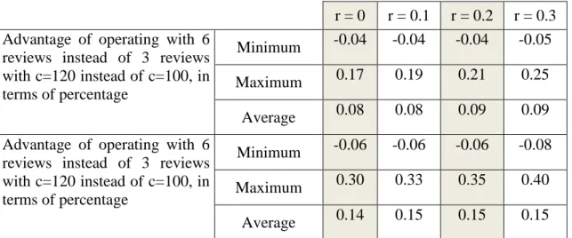
r = 0 r = 0.1 r = 0.2 r = 0.3 Advantage of operating with 6

reviews instead of 3 reviews with c=120 instead of c=100, in terms of percentage

Minimum -0.04 -0.04 -0.04 -0.05

Maximum 0.17 0.19 0.21 0.25

Average 0.08 0.08 0.09 0.09

Advantage of operating with 6 reviews instead of 3 reviews with c=120 instead of c=100, in terms of percentage

Minimum -0.06 -0.06 -0.06 -0.08

Maximum 0.30 0.33 0.35 0.40

Average 0.14 0.15 0.15 0.15

Table 4. 7 Extra advantage of shortening period length of items when purchased cost instead of , in terms of percentage

From Figure 4.3 and 4.4 it can be concluded that the advantage depends on unit holding and unit shortage cost. The advantage of operating with high unit cost item is lost as the difference between unit holding and unit shortage cost decreases. The reason can be explained with value of return information. The return information is used to prevent backordered cost. When the difference between shortage cost and holding cost decreases, the value of the return information also decreases. In these cases value of return information takes its minimum value and the advantage that can be gained by using return information is insignificant. There are some cases that the advantage of operating with low unit cost item is higher. Because the value of return information can be assumed insignificant and lower unit cost yields lower total cost, hence the advantage in terms of percentage is greater for lower unit cost items. The same claims are valid for the analyses that are conducted by disregarding sunk cost. The summary of results can be found in Table 4.8.

(50)

39

r = 0 r = 0.1 r = 0.2 r = 0.3 Advantage of operating with 6

reviews instead of 3 reviews with c=120 instead of c=100, in terms of percentage

Minimum -0.08 -0.09 -0.11 -0.23

Maximum 0.38 0.49 0.65 1.08

Average 0.17 0.21 0.27 0.41

Advantage of operating with 6 reviews instead of 3 reviews with c=120 instead of c=100, in terms of percentage

Minimum -0.12 -0.14 -0.17 -0.34

Maximum 0.65 0.83 1.09 1.77

Average 0.30 0.37 0.46 0.66

Table 4.8 Extra advantage of shortening period length of items when purchased cost instead o f , in terms of percentage

4.3.3 Analyses related to switching from no return case to return cases

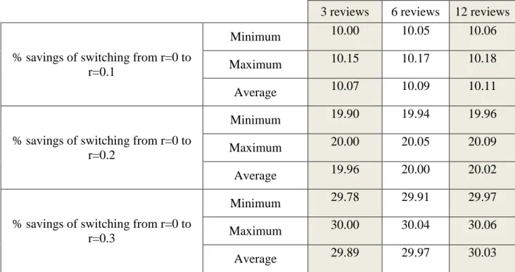
4.3.3.1 Analysis of percentage of savings with switching from no return case to return cases for all period lengths

Finally, we explore the relation between return proportion and advantage of operating with more review periods. In this analysis, the cases where are used as a base case to identify which number of period is most advantageous for switching no return case to return cases. Then the formula for calculating the percentage of savings of switching no return case to return cases for a defined period length is as follows;

(51)

40

Let us consider Case 1 in Table A.9, the total cost is 16134 where and number of period is 3. Case 1 in Table A.10 has the same parameter set except rather than 0 and its total cost is 14515. Then percentage of savings of switching from to for 3 review period problem environment with is

In Table 4.9, the summary of results can be found for all period numbers and return proportions.

Switching no return case to return case always yields positive gain, independent from return proportion. The percentage of realistic savings of switching from to is the most advantageous cases for all period numbers. This percentage is proportional to the number of review periods hence the percentage of saving is maximized when and period number is equal to 12.

In previous analysis expected total costs contain sunk cost. In Table 4.10, the summary of results that disregards sunk cost can be found for all period and return proportion. The formula to calculate percentages is as follow.

) The characteristic of results in Table 4.10 are the same with results in Table 4.9 Therefore previous claims are valid for these results. Only difference between two analyses that is worth to be mentioned is by disregarding sunk cost we eliminate the cost which is inevitably part of the total cost. Therefore the effect of switching no return case to return case is magnified.

(52)

41

3 reviews 6 reviews 12 reviews

% savings of switching from r=0 to r=0.1

Minimum 10.00 10.05 10.06

Maximum 10.15 10.17 10.18

Average 10.07 10.09 10.11

Minimum 19.90 19.94 19.96

Maximum 20.00 20.05 20.09

Average 19.96 20.00 20.02

Minimum 29.78 29.91 29.97

Maximum 30.00 30.04 30.06

Average 29.89 29.97 30.03

(53)

42

% realistic savings of switching from r=0 to r=0.1

Minimum 21.84 21.98 22.07

Maximum 22.25 22.30 22.31

Average 22.03 22.14 22.21

Minimum 43.02 43.37 43.60

Maximum 44.22 44.26 44.31

Average 43.65 43.86 44.00

Minimum 64.28 64.82 65.21

Maximum 66.31 66.44 66.49

Average 65.38 65.74 65.98

(54)

43

4.3.3.2 Analysis of switching from no return case and 3 review periods to return cases with 12 review periods

In this sub-section, we make a comparison very similar to the analysis in 4.3.3.1. We investigate the effects of using advantage of return information together with increasing review frequency. Therefore, the cases with 3 periods with no returns are taken as a base case and the cases with 12 periods with returns are used for comparison. The results can be found in Table 4.11.The formulation that is given in 4.5 is used as follow to calculate the percentages of savings.

The same analysis is conducted by disregarding sunk cost. The summary of results can be found in Table 4.12. In this case formula 4.7 is modified as follow.

For both tables Table 4.8 and Table 4.12, the percentage of saving is maximum on the average when switching is from 3 period to 12 period and to . The result that is represented in Table 4.11 (4.12) can be compared with the result in column 3 of Table 4.9 (4.10). Table 4.7 (4.10) solely represents the advantage of switching from no return case to return cases. In Table 4.11 (4.12), there is an additional factor that increases the percentage of savings and this is the increase in frequency of the review.

(55)

44

12 period

% savings of switching from 3 reviews r=0 to 12 reviews r=0.1

Minimum 10.16

Maximum 10.75

Average 10.44

Minimum 20.09

Maximum 20.60

Average 20.32

Minimum 30.11

Maximum 30.50

Average 30.29

(56)

45

12 period

% realistic savings of switching from 3 reviews r=0 to 12 reviews r=0.1

Minimum 22.47

Maximum 23.33

Average 22.85

Minimum 44.08

Maximum 44.88

Average 44.46

Minimum 65.62

Maximum 66.67

Average 66.26

Table 4. 12 Summary of results % realistic savings of switching from 3 reviews with r=0 to 12 reviews with various return proportions

(57)

46

4.3.4 Analysis of using optimal order up to levels of no return case in a return case

In this analysis is conduct to identify the increase in total cost if optimal order up to levels of no return case is used in a system where consumer returns are occurred. In other words, the order up to levels are decided under the assumption of there are not consumer returns, but consumers return some items that can be resold at the next period. By not taking returns into consideration in decision level, system is operated with order up to levels that are not optimal for the system. In this analysis, we investigate the increase in total cost, in other words loss of not operating optimally. The summary of results can be found in Table 4.13. The formula of loss of not operating optimally is as follow;

The same analysis is conducted by disregarding sunk cost. The summary of results can be found in Table 4.14. In this case formula 4.7 is modified as follow;

(58)

47

From Table 4.13 ve Table 4.14, it can be concluded that percentage of loss is maximum when , because the amount of returned that is ignored during calculation of optimal order up to levels is highest when

These results can be interpreted as what is the penalty or extra cost of not acting optimally. When order up to points are decide according to where system actually has return proportion 0.1, the loss is around %1.3 of total cost for all period lengths. This percentage increases with return proportion and it is around %6 for and %11 for .

(59)

48

% loss of not operating optimally when r=0.1

Minimum 0.39 0.39 0.37

Maximum 1.86 2.17 2.39

Average 1.23 1.32 1.33

Minimum 0.94 0.88 0.93

Maximum 5.75 6.22 6.50

Average 3.82 3.75 3.97

Minimum 1.65 1.67 1.45

Maximum 10.82 11.39 11.79

Average 7.24 7.44 7.10

(60)

49

% realistic loss of not operating optimally when r=0.1

Minimum 0.99 0.99 0.94

Maximum 4.65 5.44 6.00

Average 3.09 3.33 3.38

Minimum 2.98 2.78 2.97

Maximum 17.54 19.13 20.07

Average 11.84 11.70 12.42

Minimum 7.59 7.72 6.60

Maximum 46.58 49.62 51.87

Average 31.97 33.21 31.96

(61)

50

4.4. Importance with respect to return policy application

In this section, we sum up the results of the analyses in terms of return policy. In the analyses that are conducted over total costs including sunk cost percentage of savings and advantage of operating with more review periods is smaller than the cases which exclude sunk cost. The result of both cost structures implies same outcomes. The percentages of savings are interpreted as upper bounds because in the problem environment remanufacturing costs are disregarded. Hence, in the environment that considers remanufacturing cost there is a chance to get smaller percentages.

There is another point that needs to be emphasized. That is when number of review period is increased, the number of returned item that are resold increases as well. Because returns that are related to last review period sales are disregarded so when the length of the review period is longer, sales is higher which means amount of returned items is higher. By disregarding last period returns, the amount of returns that are disregarded in long review period environment is higher than short review period environment.

The first outcome of our analyses is that if an inventory system already adopts return policy then increasing frequency of review yields higher savings in terms of percentage.

The second outcome is operating with more review periods in a fixed time horizon is generally more advantageous for items that have high unit purchase cost instead of items that have low unit purchase costs. This advantage is lost as the difference between unit holding and unit shortage cost decreases.

The last outcome is that allowing consumer returns in an inventory system yield positive savings in terms of cost. The magnitudes of savings depend on the number of period, review frequency, in time horizon where time horizon is assumed to be a fixed length. The percentage of savings is higher when review frequency takes its maximum value. The percentage of savings is maximized when review frequency and return proportion is high.