Many-body properties of one-dimensional systems with contact interaction

O N E -D IM E N S IO N A L S Y S TE M S W ITH

TMES8S

S U B ÎV JIT T E Ö T O T H E OEPÄRTf*ÄEM T O F P H Y S İC S

A N D T H E S N S T i’

O F E N G IN E E R IN G A N D S C i

O F DSLiCEMT Ü N S V E R S IT Y

IN P A R T IA L FULFSLLfsAENT O F T H E R E O U IR E I^ E N T S

F O R T H E D E G R E E O F

¡A S T E R O F S C IE N C E

/3S3

M A N Y - B O D Y P R O P E R T I E S O F

O N E - D I M E N S I O N A L S Y S T E M S W I T H

C O N T A C T I N T E R A C T I O N

A THESIS

SUBMITTED TO THE DEPARTMENT OF PHYSICS AND THE INSTITUTE OF ENGINEERING AND SCIENCE

OF BILKENT UNIVERSITY

IN PARTIAL FULFILLMENT OF THE REQUIREMENTS FOR THE DEGREE OF

MASTER OF SCIENCE

By

Ekrem Demirel

September 1999

VJ â (VC ‘ EL·

b u t

I certify that I have read this thesis and that in my opinion it is fully adequate, in scope and in quality, as a dissertation lor the degree of Master of Science.

Assoc. Prof. Piled Tanatar (Supervisor) I certify that I have read this thesis and that in my opinion it is fully adequate, in scope and in quality, as a dissertation lor the degree of Master of Science.

Prof. Atilla Ercelebi

I certify that I have read this thesis and that in my opinion it is fully cidequate, in scope and in quality, as a dissertation for the degree of Master of Science.

Approved for the Institute of Engineering and Science:

Prof. Mehmet Baray,

A b stract

M ANY-BODY PROPERTIES OF ONE-DIMENSIONAL

SYSTEMS WITH CONTACT INTERACTION

Ekrem Demirel

M. S. in Physics

Supervisor: Assoc. Prof. Bilal Tanatar

September 1999

The one-dimensional electron systems are attracting a lot of interest because of theoretical and technological implications. These systems are usually fabricated on two-dimensional electron systems by confining the electrons in one of the remaining free directions by using nanolithographic techniques. There are also naturally occuring orgnanic conductors such as TTF-TCNQ whose conductivity is thought to be largely one-dimensional. The one-dimensional electron systems are important theoretically since they constitute one of the simplest many-body systems of interacting fermions with properties very different from three- and two-dimensional systems. The one-dimensional electron gas with a repulsive contact interaction model can be a useful paradigm to investigate these peculiar many-body properties.

The system of bosons are also very interesting because of the macroscopic effects such as Bose-Einstein condensation and superfluidity. Another motivation to study one-dimensional Bose gas is the theoretical thought that one-dimensional electron gas gives boson gas characteristics. This work is based on the study of correlation effects in one-dimensional electron and boson gases with

repulsive contact interactions. The correlation effects are described by a local- field correction which takes into account the short-range correlations. We use Vashishta-Singwi approach to calculate static correlation effects in one­ dimensional electron and boson gases. We find that Vashishta-Singwi approach gives better results than the other approximations.

We also study the dynamical correlation effects in a one-dimensional electron gas with contact interaction within the quantum version of the self-consistent scheme of Singwi et al. (STLS) We calculate frequency dependent local-field corrections for both density and spin fluctuations. We investigate the structure factors, spin-dependent pair-correlation functions, and collective excitations. We compare our results with other theoretical approaches.

K eyw ords: One-dimensional electron gas, Bose gas, contact interaction, correlation effects, local-field correction, STLS approxima­ tion, Vashishta-Singwi approximation, structure factors, pair- correlation functions, collective excitations

ö z e t

DOKUNM A

TEK BOYUTLU

SİSTEMLERİN ÇOK PARÇACIK ÖZELLİKLERİ

Ekrem Demirel

Fizik Yüksek Lisans

Tez Yöneticisi: Doç, Dr. Bilal Tanatar

Eylül 1999

Tek-boyutlu elektron sistemleri teorik ve teknolojik bağlantılarından dolayı çok ilgi çekmektedir. Bu sistemler, genellikle nanometre derecesinde yarıiletken yapı teknolojisini kullanarak, düzgün iki boyutlu elektron sistemlerindeki elektronların hareketlerinin bir boyuta sınırlandırılmasıyla elde edilir. Doğal olarak bulunan TTF-TCNQ gibi organik iletkenler de tek-boyutlu elektron sistemi özelliğini göstermektedir. Tek-boyutlu elektron sistemleri teorik açıdan da önemli; çünkü iki ve üç-boyutlu elektron sistemlerinden çok farklı özellikler göstermektedirler. Dokunma etkileşimli tek-boyutlu elektron gazı modeli bu değişik çok parçacık özelliklerini incelemek için iyi bir örnek olabilir.

Boson sistemleri de Bose-Einstein yoğunlaşması, süper-akışkanlık gibi özel­ liklerinden dolayı çok ilginçtir. Tek-boyutlu boson gazı problemini çalışmak için diğer motivasyon tek-boyutlu elektron sisteminin Bose gazı özellikleri göstermesidir. Bu çalışma, dokunma etkileşimli tek-boyutlu elektron ve boson gazlarındaki korelasyon etkilerinin incelenmesi üzerine kuruldu. Korelasyon etkileri kısa menzilli korelasyonları dikkate alan yerel alan düzeltmesiyle belirtildi.

Bu çalışmada tek-boyutlu elektron ve boson gazlarındaki statik korelasyon etkilerini hesaplamak için Vashishta-Singwi yaklaşımını kullanıyoruz. Vashishta- Singwi yaklaşımının diğer yaklaşımlardan daha iyi çalıştığını gösterdik.

Tek-boyutlu, dokunma etkileşimli elektron gazındaki dinamik korelasyon etkilerini kuvantum STLS yöntemini kullanarak inceliyoruz. Frekansa bağlı yerel alan düzeltmelerini yoğunluk ve spin uyarımları için hesapladık. Yapı faktörlerini, spin’e bağlı çift korelasyon fonksiyonunu ve kollektif uyarımları inceledik. Sonuçları diğer teorik yaklaşımlarla karşılaştırdık.

Anahtar

sözcükler: Tek-boyutlu elektron gazı, Bose gazı, dokunma etkileşimi,

korelasyon etkileri, yerel-alan düzeltmesi, STLS yaklaşımı, Vashishta-Singvvi yaklaşımı, yapı faktörleri, çift korelasyon fonksiyonları, kollektif uyarımlar

A cknow ledgem ent

I would like to express my deepest gratitude to my supervisor Assoc. Prof. Bilal Tanatar for his supervision to my graduate work. His invaluable comments and fruitful discussions we had, have been very illuminating to me in this work.

I would like to thank Kaan Güven and Mehmet Bayındır for their moral and academic support. I wish to thank Ibrahim Kimukin for his help in writing this manuscript. I also appreciate the other members of the Department of Physics, Bilkent University in the course of this study.

C on ten ts

A bstract i

Özet iii

Acknowledgem ent v

Contents vi

List of Figures vii

1 Introduction 1

2 Theory 6

2.1 Model Dielectric Functions... 6

2.1.1 Random Phase Approximation (RPA) 6

2.1.2 Hubbard A pproxim ation... 8 2.1.3 STLS A pproxim ation... 8 2.1.4 Quantum STLS A pproxim ation... 10

2.1.5 Vashishta-Singwi Approximation 13

2.2 Tomonaga-Luttinger L iq u id s... 15

3 Correlations in O ne-dim ensional System s 19

3.1 Correlations in a one-dimensional Bose gas with short-range

in teractio n ... 19

3.2 Correlations in a one-dimensional Fermion gas with short-range in teractio n ... 29

3.2.1 Vashishta-Singwi Approach 29

3.2.2 Quantum STLS A p p ro a c h ... 36

4 Discussion and Concluding remarks 46

List o f Figures

2.1 Normalized polarization function in one, two and three dimensions 7 •3.1 The ground state energy e(j) for ID boson ga.s... 22 3.2 The chemical potential, averiige kinetic and potential energies for

ID boson gas... 23 3.3 The velocity of sound Vg for ID boson gcis... 26 3.4 The static structure factor S(q) for ID boson gas in various

approximations... 27 3.5 The pair-correlation function at zero separation ¿r(0) for ID boson

gas... 28 3.6 The pair-correlation function g(r) for ID boson gas... 29 3.7 The ground-state energy per particle £(7) tor ID electron gas. . . 32 3.8 The chemical potential, average kinetic and potential energies for

ID electron gas... 33 3.9 The compressibility k for ID electron gcis. 34 3.10 The pair-correlation function ff(r) for ID electron gas... 35 3.11 The pair-correlation function at zero separation for ID electron gas. 35 3.12 The static structure factor S(q) within the qSTLS, static STLS,

GRPA, and RPA for (a) 7 = 2 and (b) 7 = 5... 37 3.13 The static spin-density structure factor S(q) within the qSTLS,

static STLS and R P A ... 38 3.14 The pair-correlation function g('r) within the qSTLS, static STLS

cind G R P A ... 39

3.15 The spin-dependent pair-correlations (j\]{r) and ,</|j(r) obtained from g(r) and ga('r') within the c|STLS. The inset compares the qSTLS and static STLS results... 40 3.16 The real and imaginary parts of the density and spin local-field

factors... 41 3.17 The large and zero frequency limit of the dynamic local field factor

G{q,i^)... 42 3.18 The disiDersion of the collective modes for (a) density fluctuations

LOd(q) and (b) spin fluctuations iOs(q) in different theories... 44

C h ap ter 1

In tro d u ction

Low dimensional systems where the motion of electrons are restricted to move in less than three spatial dimensions ai’e attracting a lot of interest because of theoretical and technological implications. The low-dimensional Coulomb gas, a system of electrons interacting in a strictly two-dimensional universe has been widely studied theoretically and experimentally.' This subject is now also an active research area because of the new and important subjects such as quantum Hall effect, metal-insulator transition. One-dimensional (ID) electron systems are also very important, because of their applicability to naturally occurring organic conductors, artificially fabricated semiconductor structures, and certain materials exhibiting superconductivity.

Recently it has become possible to create ID electronic systems experimen­ tally. These systems are usually fabricated on high-quality two- dimensional electron systems by confining the electrons in one of the remaining free directions through ultra-fine nanolithographic patterning.^ The edge states in the fractional quantum Hall effect represent another system showing more or less strictly ID properties.^’'* The motion of electrons confined to move freely only in one spatial dimension gives rise to a variety of novel phenomena, such as the non-Fermi liquid characteristics.®”^ Interacting electrons in three and two dimensions are well described by the so-called Fermi· liquid theory.® The central concept is the existence of quasi-particles which are obtained from the non-interacting electrons

Chapter 1. Introduction

by incorporating interactions into their properties. The existence of quasiparticles is reflected in a finite jump of the momentum distribution at .

In one dimension (ID), interaction between the electrons leads to peculiar properties that cannot be described within the framework of Fermi liquid theory.®’^ In one dimension, the concept of quasi-particles fails, the momentum distribution is a continuous function, and the elementary excitations are charge and spin fluctuations. The corresponding correlation functions show distinct anomalies and non-universal power-law behaviors. The Tomonaga-Luttinger modeF“^ is an exactly solvable model of ID interacting electrons within which these particular features can be treated in an exact manner.

Transport properties of one-dimensional electron systems give evidence for the peculiar behavior of Tomonaga-Luttinger liquid. The conductance quantization was obtained in short quantum wires experimentally.^’^® This result can be explained with Tomonaga-Luttinger liquid model of quantum w i r e s . O g a t a and Fukuyama also showed that the collapse of the quantization of conductance with the effect of impurity scattering for longer wires at low temperatures.^^ There are also results from Raman scattering and photoluminescence experiments on one- dimensional electron systems which can be explained by Fermi liquid theory. In Tomonaga-Luttinger liquid theory of one-dimensional systems the momentum distribution is continuous through the Fermi momentum k^r, but luminescence experiments show a discontinuity in momentum distribution at the Fermi momentum k^.^^ Hu and Das Sarma^® explained that impurity effects can suppress Luttinger liquid behavior in semiconductor quantum wires so that Fermi surface appears in real quantum wires.

The homogeneous electron gas is defined as the collection of free electrons which interact via the Coulomb law. The positive ions are at rest and smeared out so that the electrons move against a rigid uniform positive background. When the electron gas has sufficiently high density, the total kinetic energy is larger than the potential energy of the system. In this case, the system behaves like a gas of charged fermions. In the low density case, the potential energy dominates, and in the ground state the electrons are expected to form a regular

Chapter 1. Introduction

lattice which is called the Wigner ci’ystal. In the intermediate region of electron densities there are some approximations to calculate the exchange and correlation effects. The exchange effects due to Pauli principle acting to keep electrons with same spin apart was firstly taken into consideration by the Hartree-Fock approximation. The correlation effects due to Coulomb interactions in electron gas is considered firstly in random phase approximation (RPA).^^”^® Hubbard introduced a local field correction factor to the RPA and his curious formula is regarded as an improvement to the RPA in many properties. Singwi, Tosi, Land and Sjolander^^ introduced self consistent approach to calculate the local field correction factor. Their approach is called STLS approximation and it is a widely used method to calculate the properties of electron gas. The STLS approximation makes use of the one particle distribution function in deriving the density response of the many-body system to an external perturbation.^® Since the equation of motion of the one-particle distribution function depends on the two particle distribution function, two particle distribution function depends on three particle distribution function, and so on, the hierarchy of equations is truncated by making an assumption for the two-particle distribution function. Vashishta and Singwi^® then proposed a similar approach introducing a slightly different assumption at the truncation level. The instantaneous pair-correlation function is approximated as the equilibrium pair-correlation function and a term involving its derivative with respect to the density which amounts to a first order correction in the density fluctuation Sn. The local-field factor introduced in the STLS scheme to describe the correlation effects depends on the wave vector only. This is because the classical distribution functions were used in its original derivation. A quantum version of the STLS approach (qSTLS) was developed by Hasegawa and Shimizu^“ that gives a frequency dependent local-field factor. A detailed numerical calculation for dynamic correlation factor was later given by Holas and Rahman^^ for three-dimensional electron gas.

A system of bosons in one-dimension interacting via repulsive contact potential (a short-range, delta-function potential) has been a useful model to study the nature of ground state properties of quantum systems and assessing

Chapter 1. Introduction

the role played by statistics in comparison to the corresponding system of ID f e r m i o n s . T h e close analogy between the fermions and bosons in ID has been established.^^ An exact analysis of the ground-state properties of a ID interacting Bose gas was provided by Lieb and Liniger^^’^® using Bethe ansatz method. Yang^^ used the same method for the problem of one-dimensional fermions interacting via a repulsive 6 function potential. Friesen and Bergersen^® numerically solved Yang’s equations^^ to calculate the ground-state energy of the system and compared them with the STLS results. Recently, Kerman and Tommasini^^ introduced a Gaussian time-dependent variational principle for bosonic systems and applied their method to the problem of one-dimensional boson gas interacting via a repulsive contact potential. Correlation effects in a quasi-one-dimensional charged Bose condensate was also studied within the STLS a p p ro a c h .T h e re is an increasing interest in low density Bose gases because of the recent experimental progress in achieving Bose- Einstein condensation in atomic vapors under external p o t e n t i a l s . I t is expected that by adjusting the confining potential in these atomic systems, two- or one-dimensional boson condensates may be produced. Recently, the existence of Bose-Einstein condensation in a one-dimensional interacting system due to power-law trapping potentials has been shown theoretically.^”

We used Vashishta-Singwi approximation to investigate various properties of one-dimensional electron and boson systems interacting with a repulsive short-range p o t e n t i a l . W e found that the ground state energy is in good agreement with the exact result up to intermediate coupling strengths, showing an improvement over other related approximations. We also calculated the compressibility, the static structure factor, and pair-correlation function within the same approximation. The compressibility sum-rule is satisfied more correctly in Vashishta-Singwi approximation than STLS approximation. We also used the quantum STLS method to calculate the dynamical correlation effects for one­ dimensional fermion gas interacting with a repulsive 8 function p o t e n t i a l . W e investigated frequency dependent dynamic structure factor. We also calculated the dynamical spin correlation effects for the same system.

Chapter 1. Introduction

The outline of the work will be as follows. In the next section we will give some theoretical background for our work. The third chapter includes our results about the correlation effects in one-dimensional electron and Bose gases with short-range interactions. In the last chapter we summarize the results with a brief discussion of our results.

C h ap ter 2

T h eory

2 .1

M o d e l D ie l e c t r ic F u n c t io n s

One of the most basic quantities for an electron system is its dielectric function. This is determined as a linear response of this system to a test charge. The exact dielectric function for the homogeneous electron gas has not been derived yet. There are some approximate models to calculate it. I will give background information about some of these models which are important.

2.1.1 Random Phase Approximation (RPA)

The dielectric function determines screening of the long-range Coulomb potential, which in turn characterizes electronic properties of the system. Its explicit form has been evaluated in the random phase approximation. (RPA)^^ The approximation acquired its name on the basis of the physical argument that under suitable circumstances a sum of exponential terms with randomly varying phases could be neglected compared to N. In this approximation, the density of the induced charges is evaluated as a linear response of the ideal case in which Coulomb interaction is absent. The free particle polarization function (Linhard function) in the RPA is defined as^^

/(& + ,) - m ) Xo(q,u>) =

2 J

ik+q “ ^

6

Chapter 2. Theory

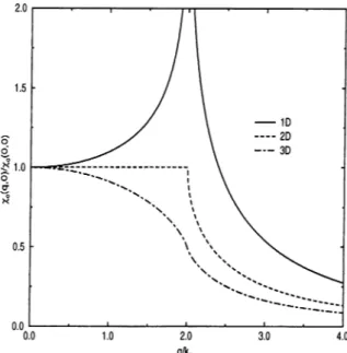
Figure 2.1; Normalized polarization function in one, two and three dimensions where rj is infinite-small number to avoid divergence in the integrals, /(^k) is the Fermi distribution function, and ^k is the kinetic energy of an electron with wave-vector k. The function Xo{q,Lo) depends on the dimensionality. In the static limit, it is real and is given by

Xo(?,0) = ^ kp 2'K^ X 27T ’ J_ 27T ^ In 2'Kq 1- (1 -1/2 q < 2 , q > 2 3D 2D ID (2.2) P-2f I ’

where q = q/kp. Fig. (2.1) shows the ratio Xo(q, 0)/xo(0,0) for one, two and three dimensions. At q = 2kp, Xaiq, 0) diverges in ID, shows a kink in 2D, and changes its curvature in 3D. The density response function of interacting electron gas in RPA is given by

■^RPAt \ _ XoCQ)^) /« o'.

Collective modes are defined as the poles of the density response function. The RPA dielectric function for electron gas is defined as

Chapter 2. Theory

2.1.2 Hubbard Approximation

Hubbard improved the RPA by taking account of short-range exchanges with a diagrammatic approach. He introduced a correction factor to the RPA of the form ^(q)Xo(q,u;) = 1 -1 -b P (q )G '(q )x o (q ,^ )’ where , 1 r(v /q ^ + k l ) = 2 - V ( q ) ■ (2.5) (2.6) The factor G{q) is introduced to account for the existence of the exchange hole around the electron. Because of the exchange hole around each electron, when one electron is participating in the dielectric screening, others are less likely to be found nearby. The factor G{q) introduced by Hubbard have an effect to reduce the electron-electron interactions. Hubbard’s expression is the simplest approximation for the calculation of local field correction.

2.1.3

STLS Approximation

The dielectric function of an electron gas both in the random-phase approxi­ mation (RPA), and the one proposed by Hubbard, which takes exchange effects into account, leads to an overestimate of the short-range correlations between particles. In this models, the pair correlation function is negative for small interparticle separations over the whole range of metallic densities and this implies an overestimate of the correlation energy. In STLS theory, an improved expression of the dielectric function is given, which includes the short-range correlations arising from both Coulomb and exchange effects by being a functional of the structure factor. The structure factor and the dielectric function can then be determined in a self- consistent manner.

We will include the method of original derivation of STLS method, given in the paper by Singwi, Tosi, Land and Sjolander.^^’^® The equation of motion for the classical one-particle distribution function /( x , p; t) in the presence of an

Chapter 2. Theory

external potential V^a;t(x, t) is

p; t)

dt + V · V x / ( x , p; t) - V xK ri(x, 0 · V p / ( x , p; t)

- y V xF (x - x') · V p /(x ,p ;x ',p '|i)c? x 'c ip '= 0. (2.7) Where l^(x) is the Coulomb interaction potential and /( x , p; x', p '|t) is the two particle distribution function. The equation for the two-particle distribution contains the three-particle distribution function, and so on. We terminate this infinite hierarchy of equations by making the ansatz

/(x. PI x'. p'lO = /(x. p; 0 /(x'. p'l 0 s(x - x')> (2.8) whei'e g{'s.) is taken to be the equilibrium static pair correlation function. This ansatz takes care of short-range correlations between the particles through the static pair correlation function ^(x). If we write

/ ( x , p; t) = /o(p) -I- / i ( x , p; t), (2.9)

where /i(x , p; t) denotes the deviation from the equilibrium distribution function /o(p) induced by the weak external potential, we can linearize Eq. (2.7) and obtain the following equation for /i(x , p;i):

( ^ + V · Vx j /i(x , p; t) - (VxK^i(x, t)

-h J 5t(x - x')V xE (x - x ')/i(x ',p ';t)d x 'd p ')V p /o (p ) = 0. (2.10) It is apparent that the effective electric field felt by a particle is

Ee//(x,t) = -W^Veff{x,t) -

J

- J [ g { x - x ' ) - l ] ' ^ x V { x - x ' ) f i { x ' , p ' ; t ) d x ' d p ' , (2.11) where the first two terms correspond to the usual macroscopic electric field, and the third term corresponds to the local field correction. In RPA, the third term is not taken into account. We can find the solution of Eq. (2.10) by considering a single Fourier component of the external potential:

Chapter 2. Theory 10

where rj is a positive infinitesimal constant. After some algebra, we obtain the induced charge density

Xo(q,t^)

And(q,cu) =

J fi{q,LO]p)dp =

X o (q ,u ;)l/(q )[l-G (9 )]

Solving for the response function defined through the relation pind = xVext·, we find that

Xo(q,i^)

(2.14) l- X „ ( q ,u ,) V ( q ) [ l- G ( q ) ] ’

where the local field correction G{q) is given by

and yo(q,i4^) is the free electron Linhard function which is given in Eq. (2.1). 5(q) is the static structure factor which is related to the density response function with the fluctuation-dissipation theorem as

-S'(q) = — - Í dulmx(q,uj).

riTT Jo (2.16)

(2.17) The dielectric response function is given as

^ i - ^ ( q ) x o ( q i ^ ) [ i - g ( q ) ]

> l + G'(q)E(q)xo(q,u;) '

Equations (2.14) and (2.15), together with Eq. (2.16), provide a set of equations which have to be solved self-consistently. These can be done starting from the known expression of ¿"(q) in the Hartree-Fock approximation, we calculate firstly the local field correction using Eq. (2.15), then we calculate a better static structure factor using the expressions (2.14) and (2.16), and so on. About 10 iterations are enough to obtain convergence in G{q) within 0.1 percent.

2.1.4 Quantum STLS Approximation

Quantum STLS approximation is similar to static STLS theory. In static STLS approximation, the density response functions are obtained from classical equations of motion. In quantum STLS (qSTLS) method, density response

Chapter 2. Theory 11

functions are obtained from the quantum mechanical equation of motion for the quantum distribution function, namely, the Wigner distribution function. The equation of motion for the two-particle Wigner distribution function, in turn, involves the three-particle Wigner distribution function, and so on. This infinite hierarchy of equations is terminated by making use of the assumption similar to that of STLS theory where the two-particle Wigner distribution function is written as

/<.,.'(■·> p; !■'>?';<) = / . ( r . p, p', - r'l), (2.18) where gu,a'{\^ — r^l) is the equilibrium, static pair-correlation function for a pair of electrons with spins a and a'. In reality, must be time dependent, but to use its static value is known to be a reasonable approximation. We introduce the spin-symmetric and spin-antisymmetric distribution functions as

/d (r,p ,i) = ^ / ^ ( r , p , t ) ,

G

(2.19)

(2.20)

where n<r = 4-1 for a and — —1 for a =J,. Making use of Eq. (2.18) we can

easily write the QSTLS equations of motion for /¿(r, p, i ) and /j( r , p ,i). Using the procedure given by Hasegawa and Shimizu,^“ the density response function is obtained from the solution of equation for /d(r, p, i) by taking A{r, t) to be the electric potential Ug(r,t). This gives the density response function as

Xo{q,^)

(2.21)

K //(ç>^)X o(9,^)'

We can obtain similarly the spin-density response function from the solution of equation for /«(r, p, t) by considering the response to a weak external longitudinal magnetic field H{r, t). We obtain the spin-density response function as

X

_

^ l - V A J q , u j ) x o { q , ( ^ ) ' (2.22)

In the quantum version of the STLS approximation, 1/^(9, a;) and V^^{q,uj) are, respectively, the spin-symmetric and spin-anti symmetric effective dynamic

Chapter 2. Theory 12

potentials. They are expressed as

(2.23) and

K“,(i,o ;) = r ( , ) J ( , , a ; ) . (2.24) where G(q,oj) and J(q,Lo) are the spin-symmetric and spin- antisymmetric dynamic local-field factors given by

and ^ 1 dkxo{q,k u) V{ k) ----/ 7^--- 7---nJ-oo2x Xo{q,<^) V{q) J{q u ) ^ - r Tl J —c (2.25) (2.26) 2TT Xo{q,i^) V{q)

In the above expressions the inhomogeneous free-electron response function

χ„(,,t;c.) = 2 Γ ^ h £ ± l ¿ l L · l ( £ ^ , (2,27)

J-oo ¿TT o j —pq/m + iq

has been used, with f{q) being the distribution function for non-interacting electrons. For k = q, the inhomogeneous response function reduces to the familiar homogeneous case Xo[q,uj). S{q) and S{q) are the static density and spin-density structure factors. They are related to the x^{q,uj) and x^iq^uj) through the fluctuation-dissipation theorem as and S(q) = — - f dLOx'^{q,iLo), nir Jo S {q ) = — i doJX^{q,i<^), niT Jo (2.28) (2.29) where we have used the analytic continuation of the response function to the complex frequency plane followed by the Wick rotation of the frequency integral. Using the definition [Eq. (2.27)] of Xo(q, k-,u>) and calculating it on the imaginary frequency axis, we obtain

m

Xo(q, k] iuj) = - — In '(c.2 + r/2 -h u ;,V )^ -4 a ;V '

Chapter 2. Theory 13

where C0qk± = \qk/2m ± qkF/m\. We take ?/ to be a small positive quantity to avoid unphysical divergences. These coupled set of equations are solved by iterating between G{q,iuj) and S{q)^ which uses x ‘^{q,u>) and in turn G{qG^)i until self-consistency is achieved. Similarly, we iterate between J{q,uj) and S{q), which uses and in turn J{q,i<^), until self- consistency is attained.

2.1.5 Vashishta-Singwi Approximation

STLS approximation makes use of the one-particle distribution function in deriv­ ing the density response of the many-body system to an external perturbation. Since the equation of motion of the one-particle distribution function depends on the two-particle distribution function, and so on, the hierarchy of equations is truncated by making an assumption for the two-particle distribution function. The approach developed by Vashishta and Singwi is also based on a similar idea but introduces a slightly different assumption at the truncation level. In STLS approximation the two-particle distribution /( x , p; x', p '|i) in Eq. (2.7) is given by the ansatz

/( x , p; x', p '|t) = /( x , p; t)/(x ', p'; i)^(x, x'; t), (2.31) where for ^(x, x'; t) the equilibrium static pair correlation ^®(|x —x'|) is used. The STLS approximation introduces correlations between particles through a physical function, and assumes that in the presence of a weak external field, g{x, x'\t) is not different from 5r®(|x — x'|), which, however, is not the case.

In the Vashishta-Singwi approximation, the zero-frequency and infinite- wavelength limit of g{x, x'; t) can be written as

g{x, x'; t) = / ( | x - x'|) + 6n ^ g ^ { \ x - x'|). (2.32) where n is the number density of electrons and 6n is the static density response. Since the external field can be arbitrarily weak, in the linear response case, terms higher than first order in 6n in Eq. (2.32) do not contribute. For finite wave vector q, we shall assume the following symmetric form for g{x,x'] t):

Chapter 2. Theory 14

where n + 6n{x, t) and n + <5n(x', t) are the local densities at x and x', respectively. This choice of ^(x, x'; t) for a one-component classical plasma exactly satisfies the compressibility sum rule. That is, the isothermal compressibility derived from the limiting behavior q — 0, u; = 0 of the dielectric function e(q, cu) is the same with that obtained fi'om differentiating the pressure.

For a weak external potential we can write

/(x,p;< ) = /o(p) + /i(x,p;< ). (2.34) where /o(p) is the equilibrium distribution function and / i ( x , p ; f ) is the small deviation induced by the external potential. Using Eqs. (2.31), (2.33), and (2.34) in Eq. (2.7) and linearizing the Eq. (2.7) as in the derivation of STLS we obtain

( ^ + v · V x ) / i ( x , p ; i ) - (^VxUext(x,f) -f-

J dxV^xp{\x-x'\)Sn{x',t)^

J

E e //(x ,i) = -

J

- J

- n - ^ [ / ( |x - x'l) - 1] VxU(|x - x'\)6n{x\t)dx'. (2.38)

The first two terms on the right-hand side correspond to the usual macroscopic electric field, and the third and fourth terms correspond to the local field correction. The third term is the same as the local field correction term in STLS. The fourth term is new and corresponds to the adjustment of the pair correlation function in the presence of an external potential. Since the density derivative of the equilibrium g^{'X·) is related to the three-particle correlation function, the

Chapter 2. Theory 15

fourth term contains effects arising out of three-particle correlations. We can find the solution of Eq. (2.35) by considering a single Fourier component of the external potential After some algebra, we can obtain the induced charge density \/r^( n {t)\ (2.39) V ^ e./(q ,cv ), 1 - 0 (q )x o (q ,^ ) where 1/ \ 1 /1 ” ^ 1 / ^q^ q ‘ q^^(qO ’P M = 1 + (1 + 5 â i ) ( - - / ( 2 ^ ) 3 ,2 i/(q)

[5(q - q') -1))

^(q)Xo(q,w)

■ V

№ - q O - i ] >

and the term in the right large parenthesis was designated as G(q) in STLS. (2.42)

2 .2

T o m o n a g a - L u t t in g e r L iq u id s

Tomonaga showed that the excitations of interacting electron gas in one- dimension are approximate bosons, although the elementary particles are fermions.® He made some approximations on the Hamiltonian of interacting one­ dimensional electron gas making it exactly solvable. First Tomonaga, then Mattis and Lieb®’^® found that boson operators can be expressible as bilinear forms in fermion fields in order to solve many-body eigenstates in the Tomonaga-Luttinger models.

The Hamiltonian of interacting one-dimensional electron gas can be expressed in second quantization form as

^ =

Z)

+

Z

k ^ k

Chapter 2. Theory 16

where e{k) = h?k‘^l2m is kinetic energy and pg = J2k *^k+q/2*^>!-g/ ‘2

density operator. This Hamiltonian cannot be solved exactly and, therefore, some approximations are needed. The first important approximation is the linearization of the dispersion relation e(k) near the Fermi points. This approximation is valid in the limit of zero temperature since the particle-hole excitations are restricted to regions near the left and right Fermi points. The low-energy picture depicted here is clearly valid for a free system, but it is not clear whether the Fermi sea can survive once the interaction is turned on.

Tornonaga hrst assumed that the dispersion is given by e{k) — hvp\k\ and then introduced the following density operators

Pk — ^ ®î-A:/2^9+fc/2) g>0 Pk ~ XI ^g-fc/2®î-l-fc/2· g<0 (2.44) (2.45) We can show that these operators satisfy the below commutation relations

[pkiP-k'] — (2.46)

T,k

[pk^p-k'\ = ~-^^k,k', (2.47)

[pk 1 P-k'] — (2.48)

where k > t). These commutation relations are valid as long as the particle distribution function do not change significantly as a result of the interaction. If we define the following new set of operators, hk = / L k p ^ , h\ = 2ttj L k p ’^ij^,

b^_j^ = b-k — ILkpZk- These operators satisfy the bosonic

commutation relation [bkib\,] — 8k,k'· The new operators also satisfy the following commutations relations with the kinetic energy part of the Hamiltonian,

Hq

=

[bk,Ho]=u:kbk, (2.49)

Chapter 2. Theory 17

where u = hvp\k\. From these commutation relations, we can say that Hq is

just a system of simple non-interacting harmonic oscillators represented by the raising and lowering operators h\ and hk·, and the full Hamiltonian is given by

H = +14(6/. + + 6-»). (2.51)

where Vk = \k\Vk/2Tr. This Hamiltonian can be diagonalized by the following Bogoliubov transformation

bk — (cosh7)o;yt -I- (sinh

b\ = (cosh7)aJ + (sinh7)a_)t,

(2.52) (2.53) where 7 is a free parameter, a and are bosonic operators. If we make the identification

exp(47) =

+ 414

the interacting system can again be represented by the simple harmonic oscillators, H — Y^k ^kOi\oik·, where the dispersion is modified to Ek =

y u l + AoJk^·

As we show, in Tomonaga model there are some approximations to solve the problem. Luttinger made the various commutation relations in the Tomonaga model exact introducing two sets of operators for the left- and right-movers near the Fermi points such that they obey the following anti-commutation relation

\^k,ai ^k',a'} — ^aa'^k,k'■> (2.55)

where a is the index which changes with the direction of movers. The new density operator also acquire this index as

Pk,a — ^ (2.56)

where the sum is over all p. Unlike the Tomonaga model the Luttinger model is exactly solvable with no further approximation. Using the commutation

Chapter 2. Theory 18

relations, we can reduce the Hamiltonian for one-dimensional interacting system in Luttinger model to the form

H = Ho + Vi + V2,

where Vi and V2 is given by

r . = E W i k b i k + k>0 (2.57) (2.58) (2.59) U = E Ú(6«52,-í + bl b{ _ ,) . fc>0

The Hamiltonian H is exactly solvable because it describes linear coupling between two harmonic oscillator systems. The Luttinger model is different from Fermi liquid model in various respects. The Fermi liquid model assumes a finite density of electrons in a parabolic kinetic energy dispersion, while the Luttinger model assumes an infinite density of negative energy electrons in a completely linear kinetic energy dispersion. In Fermi liquid theory the interaction between electrons is assumed as Coulomb interaction but in Luttinger model the interaction is assumed as short-range contact potential.

Li, Das Sarma and Joynt^® showed that in the long wavelength limit the RPA plasmon disj^ersion for one dimensional electron system is almost the same with the Tomonaga-Luttinger energy dispersion relation Ek = \J<^k T 4cUfcI4 where

(jo = fiVF\k\ and I4 = \k\Vkl2-K. The plasmon dispersion of one-dimensional

system in RPA is given by the formula

tu, =

A { q ) - 1 ’

with A{q) = exp{qTTfmV(q)) and u>±= qvp ± q^/2m. If we expand Eq. (2.60) in long wavelength limit up to second order in q/kp we obtain

n l / 2

OJg = |Ç| Vp + - vp V ( q)

IT

(

.

)

We note that this is exactly the same as the eigenenegy of the elementary - excitation spectrum in the Tomonaga-Luttinger model.

C h ap ter 3

C orrelations in O n e-d im en sional

S y stem s

3 .1

C o r r e la t io n s in a o n e - d im e n s io n a l B o s e g a s

w it h s h o r t - r a n g e in t e r a c t io n

We investigated the problem of one-dimensional boson gas interacting with a contact potential V ( r i , r2) = Vo6{r\ — r2) where Vq is the interaction strength.

An exact analysis of the ground-state properties, in particular the ground-state energy as a function of the coupling strength, of a ID interacting Bose gas was provided by Lieb and Liniger.^^ Correlation effects in a ID Bose gas within self-consistent field approximation was first attempted by Hipólito and Lobo^^ and recently by Gold within STLS approximation.^* The local field cori’ected Bogoliubov approximation*^’*^ shows a definite improvement for the ground state energy. We use the Vashishta-Singwi method^^ to calculate correlation effects. We find that the exact ground-state energy*“* within this perturbation theory approach can be faithfully reproduced up to large values of the coupling constant.

In terms of the boson mass m and the density of the particles n, we define the dimensionless parameter 7 = mVofn to characterize the strength of the coupling (we take h = 1). We assume that the ID bosons are in the condensate and

Chapter 3. Correlations in One-dimensional Systems 20

the generalized Bogoliubov model is applicable. The local field concept applied by Gold using STLS approximation is quite useful in understanding the weak coupling regime of ID bosons. The ground state properties calculated within STLS scheme were in good agreement with exact results of Lieb and Liniger as 7 —>■ 0.

Vashishta-Singwi approximation^® was originally constructed to satisfy the compressibility sum-rule. As discussed in Sec. 2.1.5, in the Vashishta and Singwi model the equilibrium pair correlation function g(r) which enters the ansatz for the two-particle distribution function is amended by a correction term involving the density derivative of g{r). For a one- dimensional system of bosons interacting with a contact potential the local -field factor in the Vashishta-Singwi approximation is given by

d

Gvs(7) = 1 + an

d n , — Í d q [ l - S { q ) ]n iT JO (3.1)

where a is an adjustable parameter. The local-field factor G is still independent of the wave-vector variable as in the STLS approximation. The static structure factor S{q) is given in the generalized Bogoliubov approximation by®®

- 1/2 S(q) =

r

(3.2) When we substitute Eq. (3.2) into Eq. (3.1), we obtain the following differential equation for Gvs{l)

dGvs

— 3^2 Gws (1 — G'vs)^'^^ + ^ ^ ^ (1 — G\s) , (3.3)

¿7 07· ^ / ' ' 7

which is first order but highly nonlinear. Instead of solving this equation numerically, we use an approximation given by

d

GvsÍ7) “ ( ^ j GsThsilf), (3.4)

which is a lowest-order expression in the iterative solution of Eq. (3.1) and Eq. (3.2) starting from the STLS solution. We can obtain the Gs t l s{i ) using

Chapter 3. Correlations in One-dimensional Systems 21

Eq. (3.2) in Eq. (3.1) for the parameter a=0 as^®

f?STLs(7) = (1 + ~ 1 ? (3-5)

and using Gstls in Eq. (3.4) we obtain Gvs ns

Gvsi l) = - ^ ( l - a ) 7 [(1+ - l] + a (1 + Tr^/7)“ ^/^ . (3.6) In the Vashishta-Singwi theory^^ the parameter a is determined by adjusting the compressibility calculated using the ground state energy and that obtained from the long-wavelength limit of the dielectric function. In this work we take a = 1/2 which gives the best agreement with the exact ground state energy.

The differential equation which is given in Eq. (3.3) can be transformed to Riccati equcition.‘‘° In this transformation, we first define 1/(7) = (1 — 6^(7))^/^ and then dividing the equation by «(7) we obtain the Riccati equation u'(7) = -f c(7)u(7) + ¿(7) where 6(7) = 7r/2a7^/^, 0(7) = (2 — a)/2'y and (¿(7) = —7r/2a7^'^^. The Riccati equation can be transformed to linear second order differential equation for 00 by the transformation u(7) = u)'{j)/{u>{'j)b{'y)).

Then one can obtain Gvsi'j) explicitly. ^

Ground State Energy

The interaction energy per particle of a many particle system is written as 1

(3.7) in which the Hartree contribution is also included. Within the mean-field theory this reduces to

Eintil) = ^ [1 “ - <^(7))^^V’t] · (3.8) The ground state energy per particle is calculated by a coupling constant integration

Eo = r d X E i n t W / X . (3.9)

Jo

Chapter 3. Correlations in One-diinensionai Systems ₂₂

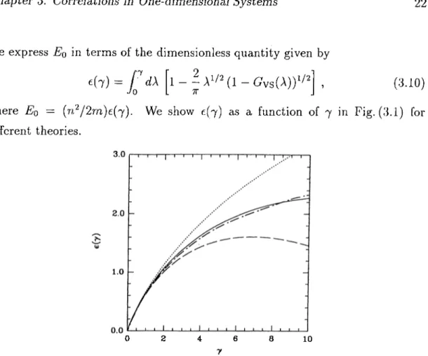
We express Eq in terms of the dimensionless quantity given by

(7) = fl - i - Gvs(A))‘'"'

•/0 L 7T (3.10)

where Eo — (n^/2m)e(7). We show £(7) as a function of 7 in Fig. (3.1) for different theories.

4 6

r

1 0

Figure 3.1: The ground state energy £(7) for ID boson gas. The dotted and dot- dashed lines are for STLS approximation and the exact result respectively. The solid and dashed lines represent the VS approximation for a = \/ 2 and a = 1, respectively.

We see that Vashishta-Singwi approximation gives a better agreement than the STLS result to the exact ground state energy £(7). In the exact treatm ent of £(7), an expansion for small 7 is not possible because of the inadequacy of the perturbation theory and non-analytic properties of £(7) as 7 —> 0. Analytic forms of STLS and VS local field correction factors gives us an opportunity to make a weak coupling expansion of £(7). Gold'^® made a weak coupling expansion of (^STLsil) esTLs(7 0) = j - — 7^^^^ -f-•JTT 1 —r 7^ ~ ----7T^ StT^ 2 5 / 2 ^ 7 ^ + (3.11)

We see from Fig. (3.1) that the STLS approximation compares well with the exact result of Lieb and Liniger^'' only for 7 < 2. We also made the following weak

Chapter 3. Correlations in One-dimensional Systems 23

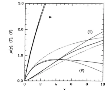
coupling expansion (for a = 1/2) evs(7 ^ 0) 7 _ ± ^ 3 / 2 ^_{37T ^ ^ 47} t2 ^ 407t^ ^5/2 _ 1927t4 73 _ 11 35847r·' 7 " " + (3.12) If we compare the weak coupling expansions of tsTLs{l) £^5(7) we see that terms of order A” where n > 3 are missing in the esTLs(7) expansion. The other ground state quantities of interest are the chemical potential p —

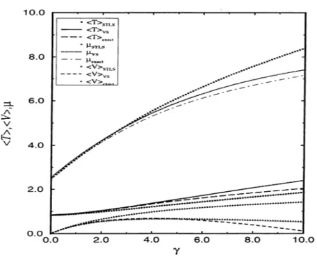
d E o/d N = (n^/2m)(3e — -fdefdj), the average potential energy per particle (V) = (n'^/2m)'yde/d'y, and the average kinetic energy (T) = Eq — {V) =

(n^/2m)(e — 'ydeld'y). Using the numerically calculated evs(7) we compare these quantities with the results of the exact solution to the ID boson problem in Fig. (3.2). We see that the STLS approximation results (dotted lines) start deviating from the exact calculation of {T) and (V) for 7 Ri 2. The VS calculation represents (T) reasonably well, but the potential energy term starts to deviate from the exact result for 7 > 6. However a cancelation effect renders the total energy in quantitative agreement with the exact result up to 7 10 (see Fig. (3.2)). In the available range of 7 both the STLS and VS approximations agree well with the exact result for the chemical potential /i(7).

The weak coupling limits of the chemical potential and the average potential and kinetic energies per particle (in units of n^/2m) in the VS approximation are given by 7 ,/o 11 2 0/0 3 ^ = 2 7 - - 7 / + — 7T 4 7 r ^ 7^ -/ T -/ \ ^ 3 / 2 ^ 2 ^ + 2 ^ 7 (T) = _ .y3/2 _ ir-ol + 21 7 SOtt^ ^ 5/2 _ 5/2^ _ 71687T® 5 , 11 647t^ 5 7 = -7® + 10247* 55 7 " " + / / 2 + (3.13) (3.14) (3.15) 37T ' 47t2 ' ' 807t^ ' ' 967t^ 71687t®

When we perform a similar calculation using the ground-state energy within the STLS approximation,^® we obtain ^ = 27 2 3 / 2 ^ 1 2 -7T 1 ( y ) = 7 - i y / * + 7T 1 75 / 2 _ 1 - . ^ 2 _ - L ^ 5 / 2 + ^ 7 T / 2 ^ 2 28TT® 1 4TT® y ‘ + (3.16) (3.17)

Chapter 3. Correlations in One-dimensional Systems 24

4 6

y

10

Figure 3.2: The chemical potential, average kinetic and potential energies for ID boson gas. The thick solid lines denote the exact results. The thin solid lines and dotted lines are for the VS and STLS approximations respectively.

(3.18) which again shows that certain terms are missing in the expansion of (F) and

{T) compared to the VS approximation.

C ollective E xcitations

The collective mode excitation spectrum in our model is readily obtained from the RPA-like density-density response function. The RPA like density response function is obtained as

Xo{q,uj) =

---and the dielectric function with local field correction is defined as Eq. (2.5). The dispersion of collective excitations co{q) is obtained by solving the equation

1 + G'(q)V(q)xo(q,i^) The solution of this equation is given by

^ ( " / " ) ' + “7(1 - G ( 7 ) ) l''^

(3.20)

Chapter 3. Correlations in One-dimensional Systems 25

which represents a gapless excitation (may be identified as the Goldstone mode). Taking G(j) = 0 or its weak coupling limit G('y) fa 27^/^/7г yields the Collective mode dispersion in the RPA and the Bogoliubov approximation, respectively. In the exact solution^“* of the interacting ID boson gas two types of elementary excitations were found, the first of which (‘particle’ excitations) corresponds to the Bogoliubov spectrum. The second type (‘hole’ excitations) of the elementary excitation which exists only for |ç| < irn, is not accounted for within the Bogoliubov cipproximation or the present model with a local-field correction. Part of the reason for this is that the Bogoliubov model assumes that all the particles are in the condensate whereas in the treatment of Lieb and Liniger^'*’^^ no such assumption is made. In the recent work of Kerman and Tommasini^^ the self-interactions of the particles out of the condensate are taken into account. Although the Gaussian variational method provides only an upper bound for the ground state energy and does not reproduce the exact energy so well for 7 > 5, it captures successfully the basic structure of the elementary excitations.

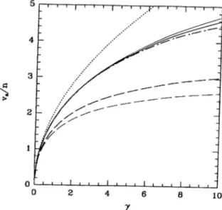
The VS theory was originally devised^® to fulfill the compressibility sum-rule in interacting electron systems. It was demonstrated that the compressibility calculated from the long-wavelength limit of the response function coincides with thcit calculated from the ground-state energy through the thermodynamic relation. Since the compressibility is also related to the velocity of sound by 1//Î = rrmUj, we can use the sound velocity in the present context to check the compressibility sum-rule. The sound velocity may be calculated from the excitation spectrum Vg = liiUg^o diOq/ dq which yields the result

Vs = 2n[47(l — G'(7))]^'^^. On the other hand, the thermodynamic relation 17n) Eofd'j'^, gives

Vs = 2 2 2^^^ o o

-1I/2

(3.22)

In Fig. (3.3) we show the velocity of sound calculated in the VS and STLS approximations using the above mentioned two different ways. The ground-state energy based calculation of Vs within the STLS and VS approximations are quite close to the exact result for 7 < 10. The excitation energy spectrum based

Chapter 3. Correlations in One-dimensional Systems 26

Figure 3.3: The velocity of sound for ID boson gas. The lower (dashed) and upper (solid) curves are calculated from the excitation spectrum and thermodynamic definition, respectively. The thick and thin lines are for the VS and STLS approximations, respectively. The exact result is depicted by the dot-dashed line. Vg calculated using the Bogoliubov excitation spectrum is given by the dotted line.

calculation of Vg remains below the thermodynamic results. In the VS approach the compressibility sum-rule is violated less than in the STLS approach, but it is still not very satisfactory. The Bogoliubov spectrum yields a sound velocity above the energy based results. It is not surprising that the compressibility sum-rule is not satisfied either in the STLS or the VS approximations, since both of these schemes assume that all the particles are in the condensate. In other words, the local-field based theories take only the ‘particle’ contribution to the excitation spectrum and neglect the ‘hole’ excitations.

Static structure factor and Pair-correlation function

The static structure factor as defined in Eq. (3.2) gives a measure of the correlation effects. For a noninteracting system it is unity and in the I’andom- phase approximation (RPA) we take G('y) = 0. The Bogoliubov approximation is recovered when the leading order term in the local-field factor is retained, viz.

Chapter 3. Correlations in One-dimensional Systems ₂₇

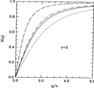
G(‘j ) = 27*/^/7t. Fig. (3.4) shows the static structure factor S(q) for 7 = 2 in the RPA, Bogoliubov, STLS and the present VS approximations.

Figure 3.4: The static structure factor S(q) for ID boson gas in various approximations. The solid and dot-dashed lines indicate S'v'5(<7) SsTLs(q),

respectively. The dotted and dashed lines are for the RPA and Bogoliubov approximations, respectively.

In the RPA the interaction effects are over-stressed. The Bogoliubov approximation is closest to the noninteracting result, but for 7 = 2 it may already be not so good. The inclusion of the local-field correction G(j) tends to decrease

S(q) from the Bogoliubov result, since in the latter correlation effects are not

fully taken into account. The probability of finding two bosons at a distance r is described by the pair-correlation function g(r) which is the Fourier transform of S(q). Performing the one-dimensional Fourier integral analytically we obtain the pair-correlation function within the present model as

gvs(r) = gvs{0) + 7*^^ (1 - GvsV^'^ [/i(2rn7^/^(l - Gvs)^^^)

- L i(2 rn 7 i/^ (1 -G 'v s )’/")], (3.23) where Ii(x) is the modified Bessel function (of the first kind), Li(x) is the modified Struve function,^® and <7vs(0) = 1 — (2/7t) 7G2 (1 _ is the pair-correlation function at zero separation. Note that a similar expression for the

Chapter 3. Correlations in One-dimensional Systems 28

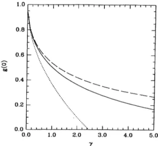
pair-correlation function within the STLS was also given by Cold.^® Figure (3.5) compares 5tvs(0) with <7stls.(0) as a function of 7.

Figure 3.5: The pair-correlation function at zero separation ^'(0) for ID boson gas. The solid, dashed, and dotted lines indicate 5fv5(0), (Js t l s(0), and ^'(0) in

the Bogoliubov approximation, respectively.

It was noted that in the STLS approximation ^(0) remains positive for all 7, unlike the Coulomb systems which yield unphysically negative 5r(0) at some intermediate coupling strength. In the case of Vashishta-Singwi approximation, we find that 5f(0) eventually becomes negative for 7 > 15. Since the theories involving the local-field factor are perturbational in character, thus limiting their applicability for small and intermediate range of 7, our result for <7vs(0) should be useful in practical applications. The weak coupling limit of 5'vs(0) is given by

lim <7vs(0) ~ 1 - -7*/^ -1- -^7(1 - a/2) -f

7—»-O 7T 7T^ (3.24)

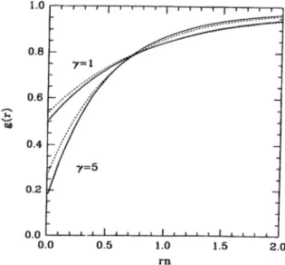
which reduces to the STLS result^® 5'stls(0) — 1 — 27^/^/7T, as a —> 0. The effect of the STLS and VS local-field corrections on the pair-correlation function is further illustrated in Fig. (3.6) where g{r) is plotted for 7 = 1 and 7 = 5, and we also specialize to the a = 1/2 case. The differences occur largely at small separations. The asymptotic forms of g{r) are obtained as

Chapter 3. Correlations in One-dimensional Systems 29

Figure 3.6: The pair-correlation function g{r) for ID boson gas. The solid and dotted lines indicate gvs{i^) and gsTLsif')·, respectively.

,9vs(^ 0) = i?vs(0) + rn7 [1 - Gvs(7 )]---- ~ G'vs(7)f^^ + · · · (3.25)

and

gvs{r· -> oo) = 1 - __2_Trr'^n"^^ 2 “ f ? v s 2 7 r Hn ‘' ~ G'vs(7)]~^^^+· (3.26) A comparison with the corresponding expansions in the STLS approximation shows that both methods have the same r-dependences.

3 .2

C o r r e la t io n s in a o n e - d im e n s io n a l F e r m io n

g a s w it h s h o r t - r a n g e in t e r a c t io n

3.2.1

V ashishta-Singw i A pproach

We considered a system of electrons in ID interacting via a contact potential

y{f'ui”2) = VoS{ri — r2), where Vq is the interaction strength. We define the

Chapter 3. Correlations in One-dimensional Systems 30

density of the particles n to characterize the strength of the coupling as like in the ID boson gas problem.

One-dimensional electron system interacting with repulsive 6 function potentiell were treated by Yang^^ using the Bethe ansatz method. Friesen and Bergersen^® numerically solved Yang’s equations^^ and calculated the ground state energy of the system as a function of 7 and compared them with STLS results. Gold“^^ used an approximate analytical expression for the static structure factor with the STLS approach and compared his results with Friesen and Bergersen’s results, where numerical results for the static structure factor are used. Within the STLS approach, the local field correction for ID electron system is given by

GsTLsh) = — / dq[l - 6'(^)], (3.27)

niT Jo

which is independent of the wave-vector variable like in the ID boson system. Using the rnean-spherical approximation^^ we can write the analytical expression for static structure factor

5(?) = _^1 4n^ , ,,

‘5o Q

- 1 / 2

(3.28) where So{q) is the static structure factor of the noninteracting electron gas in ID, i.e. So{q) = qf2kp·, for q < 2kp, and So{q) = 1, for q > 2kp· When we substitute Eq. (3.28) into Eq. (3.27) we obtain a cubic equation

1 -f 87(1 - G(7)]/7t^

G{l) = _{2 [H -4 7 [1 -G '(7 )]/7t2]i/2·} (3.29)

We solved this equation analytically. There are three different solution of this equation. However only one of them is physically acceptable.

We use the Vashishta-Singwi^® approach to calculate the correlation effects for this s y s t e m . R a t h e r than solving the highly nonlinear differential equation to calculate Gvsi'l) we make the same approximation given in Eq. (3.4), which is the lowest order expression in the iterative solution of Eq. (3.1) starting from the STLS solution. We take a = 2/3 which satisfies the compressibility sum rule best. We find that the lowest order approximation is capable of improving the STLS approach to the ground state energy remarkably.

Chapter 3. Correlations in One-dimensionai Systems 31

G ro u n d S ta te E n erg y

The interaction energy of the ID electron system can also be calculated with Eq. (3.7). Using Eq. (3.28) in Eq. (3.7) we obtain

1 + 87(1 - G(7)]/7t^

Einti'l) = {n^l2m)'y 1 (3.30)

2[l + 4 7 [ l - G ’(7)]/7r2]i/2_

The contribution of the interaction energy to the ground state energy is calculated by coupling constant integration. (Eq. (3.9)) There is also the contribution of kinetic energy to the ground state energy. The kinetic energy per particle for a ID electron system which is in ground state is given by ep/S = (7r^/12)n^/2m. We express ground state energy Eq in terms of the dimensionless quantity given

by

1 + 8A[1 - G'(A)]/7t2 ^(7) = 1 2 +

f d X l l - 2[1 + 4A[1 - G(A)]/7t2]i/2 where Eq = (n^/2?7г)e(7). The series expansion of esxLsi^) as 7

(3.31) / 1 3 2 b e W 7 ^ 0 ) = - + - 7 - ^ 7 7 _IO tt®7^* + 0 is 77 IOtt®7

and the series expansion of 6^5(7) in the same limit is

/

7^2 1

3

11

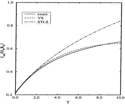
Figure (3.7) shows that the VS approach which we used here gives a better agreement than the STLS result to the exact ground state energy ^(7). We see from the series expansions that evsi l) and csTLsi'j) start to differ at the cubic term in 7. We also calculate the some other ground state quantities of interest which are the chemical potential /i, the average potential energy (V) and the average kinetic energy (T). We show the results of these quantities for three different theories in Fig. (3.8). We fist note that the STLS approximation results start deviating from the exact calculation of {T) and (V) for 7 ~ 2. The VS calculation represents (T) reasonably well, but the potential energy term starts to deviate from the exact result for 7 > 6. However a cancelation effect renders the total energy in quantitative agreement with the exact result up to 7 f« 10.

Chapter 3. Correlations in One-dimensional Systems 32

0.0 2.0 4.0 6.0

Y

8.0 10.0

Figure 3.7: The ground-state energy per particle e{j) for ID electron gas. In the avciilable range of 7 both the STLS and VS approximation agree well with the exact result for the chemical potential

C om pressibility

There are two ways to calculate the compressibility. We can calculate it from the ground state energy and density response function. Using the thermodynamic relation ^ = n'^-^{nEg), we can calculate the compressibility. Secondly, we can calculate the compressibility by using the formula limq^ox{q, 0) = —n^K, where the density response function x(?,a;) of an interacting electron gas with local field correction factor G{'y) given by Eq. (3.29). Using the thermodynamic relation we find

li·

(3.34) and the long-wavelength limit of the static density response function yields

r2

7T

Chapter 3. Correlations in One-dimensional Systems 33

Figure 3.8: The chemical potential, average kinetic and potential energies for ID electron gas.

where kq = 2/(n^7r^) is the compressibility of the noninteracting electron gas

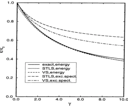
in ID. Figure (3.9) shows the compressibility calculated in the VS and STLS approximations using these two methods. The ground state energy based calculation of k within the STLS and VS approximations are quite close to the

exact result for 7 < 10. The upper and lower curves are calculated from the excitation spectrum and thermodynamic definition, respectively. The thick solid line is the result using the exact ground-state energy. The ground state energy based calculation of k within remains below the excitation energy spectrum based calculation of /c. The VS approach improves the compressibility sum-rule over the STLS result, but does not fulfill it exactly.

Pair-correlation Function

The probability of finding two electrons at a distance r is described by the pair- correlation function g(r) which is the Fourier transform of S{q). We obtain