On the set of all stabilizing first-order controllers

On the Set of

All

Stabilizing First-Order Controllers

K.

Saadaoui and

A. B.

Ozguler

Department

of Electrical and Electronics Engineering,

Bilkent University, Ankara, Turkey.

karim@ee.bilkent.edu.tr,

ozgulerQee.bi1kent.edu.tr.

A b s t r a c t

A computational method is given for determining the set of all stabilizing proper first-order controllers for finite dimensional, linear, time invariant, scalar plants. The method is based on a generalized Hermite-Biehler theorem.

Keywords: Hermite-Biehler theorem, stabilization, linear systems.

1 I n t r o d u c t i o n

In [l], a Computational characterization of all sta- bilizing proportional-integral (PI) and proportional- integral-derivative (PID) controllers was derived. In [Z], an alternative fast method for determining all stahi- lizing PID controllers was derived. The limiting values of controller parameters that guarantee stability are determined in [l] using an extension of the Hermite- Biehler theorem [3], and using the Nyquist plot in 121.

In this paper, we give an extension of the method of [l] to solve the problem of. determining all first-order controllers that stabilizes a given plant. The paper is organized as follows. In section 2, the method for cal- culating stabilizing gains is revisited. In section 3, we give an algorithm for determining stabilizing first-order controllers. Finally, section 4 contains some concluding remarks.

2 P r o p o r t i o n a l Controllers

Let C denote the set of complex numbers and let

C - , C O ,

C+

denote the points in the open left half, jw-axis, and the open right half of the complex plane, respectively. Then, the set

X

of Hurwitz stable poly- nomials are ‘H = {$(s) E R[s] : $(s) = 0 =$ s E C-}. The derivative of $ is denoted by $’ and the signa- ture U($) of a polynomial $ E R(s] is the difference between the number of its C - roots and C + roots.

Given $ E R(s], the even-odd components ( a , b ) of $(s) are the unique polynomials a , b E R[u] such that $(s) = a(.?)

+

s b ( s 2 ) . Finally, the greatest common divisor of a and b is denoted by gcd{a, b } and [ml de- notes the greatest integer less than or equal to m E R. We state the following result for later reference. The proof of this result follows by a generalization of the Hermite-Biehler theorem [3].

L e m m a 1. A nonzero polynomial $ E R[s] has r real negative roots without counting the multiplicities if and only if the signature of the polynomial $(s2)

+

s$’(s2) is 2r. All roots of $ are real, negative, and distinct if

and only if $(s2)

+

s$’(s2) E

H .

We now describe a slight extension of the constant sta- bilizing gain algorithm of [3]. Given a plant g ( s ) =

%,

where p , q E R[s] are nonzero with m = deg p less than or equal to n = deg q , the set A , ( p , q ) :=

{ a

E R :

u [ 4 ( s , a)] = u [ q ( s )

+

cup(s)] = r, deg

4

= deg q } , is the

set of all real a such that

4(s,

a) has signature equal to

r. Let ( h , 9 ) and ( f , e ) be the even-odd components of q and p , respectively. Let d := gcd {f, e } so that

f

=

d f , e = db, or coprime polynomials

f ,

E E

R[u].

Then, the polynomial

p ( s )

:= f(s2)

+

sE(s2) = p ( s ) / d ( s 2 ) is free of C O roots except possibly a simple root a t s = 0.

Let ( H , G ) be the even-odd components of q(s)p(-s). Also let F ( s 2 ) := p ( s ) p ( - s ) . By a simple computation, it follows that H ( u ) = h ( u ) f ( u ) - ug(u)E(u), G ( u ) = g ( u ) f ( u ) - h ( u ) E ( u ) , and F ( u ) = f ( u ) f ( u ) - u e ( u ) E ( u ) .

If G

p

0 and if they exist, let the real negative ze-

ros with odd multiplicities o f G ( u ) he,{vl,

...,

v k } with

the ordering v1

>

vz

>

. . ,

>

vk, with uo := 0 and

U k + l := --oo for notational convenience. The following algorithm determines whether A , ( p , q ) is empty or not and outputs its elements when it is not empty: Algorithm 1.

1. Calculate

- z ( ~ ; ) , i = 0 , . . . , k for odd r - m

{

- $ ( v , ) , i = 0,

. . . ,

k + 1 jor even 7 - rn,

ai =

and sort them in ascending order do

< 61

<

. . .

<

d k + 2

<

d b + 3 where do = -m and ( 1 k + 3 = m.

2. Identify all the sequences of signums

=

{

{ i o , i ~ , . . . , i k } for odd r - m

for even r - m, ( i o , i , , . .

.

, i k + l }

where i o E { - l , O , l } and ij E {-1,1} for j =

1 , . .

.

, k+l, that comspond to the intervals (di,

e,+,)

f o r i = 0,. . . , k

+

2.

3. For each signum sequence 1, from step 2, i j i o - 221

+ . .

.

+

2 ( - l ) k i b T - m odd

i o - . . .

+

( - l ) k + ’ i t + i r - m even. r - u ( p ) =

holds, then ( d . , a i + ~ ) E A , ( p , q )

R e m a r k 1. By step 3 of Algorithm 1, a neceS sary condition for the existence of a n a t A , ( p , q ) is 0-7803-7896-2/03/$17.00 02003 IEEE 5064 Proceedings of the American Control Conference Denver. Colorado June 4-6.2W3

that the odd part of [ q ( s )

+

a p ( s ) ] p ( - s ) bas a t least

f = max{O,

[ e l }

real negative roots with odd multiplicities. &en solving a constant stabilization problem this,lower bound is f = max{O,

['"-"~"-'l}.

3 First-Order Controllers

A

first-order controller c(s) = applied to

go(s) =

%,

with m = deg pa less than or equal to n = deg q0, gives the closed loop characteristic polyno- mial

q+i(s,ai,uz,a3) = ( s + a i ) q o ( s ) + ( o I z s + ~ ~ ) P ~ ( s )

= PI (s)

+

a3P1 (s) ( 1 )

Multiplying &(s,a1,a2,a3) by Q~(-s) we obtain

(2)

Note that a l , a2 appear in the odd part and a l , 03

appear in the even part. It is no longer possible to exploit the results given in [l] and proceed.

The reasoning behind the below algorithm can be ex- plained as follows. Suppose that 41(s is Hurwitz stable

the odd part of $1(s) has a t least T I =

1-1

real

negative roots with odd multiplicities. By Lemma 1, u[q4z(s)] = 271, where

for some 011, a2, 013 E R. By Remar

h'

1, it follows that

&(s) = H ( s Z )

+

a i C ( s 2 )

+

azF(s*) + s [ H ' ( s Z )

+

aiG'(sz)

+

a2F'(s2)]

= qz(s)

+

azpz(s)

In order to find the suitable ranges of at and az,

we modify 62f.s) as follow_s.. Let B := gcd{F,F'} so

thai

F = B F , F' = BF'_for coprime polynomials

F , F '

E

R[u].

Let p z ( s ) := F ( s 2 )

+

sF'(s2). Then, by

a straightforward computation, $ z ( s ) = + + 2 ( s ) p ~ ( - s ) =

I(sz)

+

a l J ( s Z )

+

a z K ( s Z )

+

s [ L ( s z )

+

a ~ M ( s ' ) ] , where

I ( u ) , J ( u ) , K ( u ) , L ( u ) , and M ( u ) can be easily com- puted. Once more by Remark 1, the odd part of &(s) has at least r2 = ~ J 2 r 1 - - o ( p z ) J - 1

1

real negative roots

with odd multiplicities. V&es of a1 E R achieving r2 real negative roots with odd multiplicities can be deter- mined using Lemma 1 and Algorithm 1. In Algorithm

2 below, we follow a nested procedure where one a1, a2 is determined and then the corresponding values of

013 are obtained.

Algorithm 2.

1. Using Lemma 1 and Algorithm 1, partition the real m ' s into interuals such that in every interval L ( u )

+

a i M ( u ) has a constant number of real negative roots with odd mdtiplicities.

2. Fizr1 = 1-j.

(a) Determine from step 1 if a mnge.of 01 for which 2r -(r

r2 =

11

1 ?)'-1j ezists.

i. Fiz an 011 in the mnge of step 2.a.

ii. Apply Algorithm 1 to qz(s) replacing q ( s )

,

pz(s) replacing p ( s ) , and u(dz) = 2ri re- placing r . (This calculates admissible val- ues of az such that H ( u ) + a ~ G ( u ) + a z F ( u ) has r1 real negative mots with odd multi- plicities.)

A . Fiz an a2 from the range determined

in 2.a.ii.

B. Apply Algorithm 1 t o q l ( s ) andp,(s) =

p ( s ) . (This calculates all admissible valves of a3 such that $1 of ( 1 ) is in H . 1

C. Increment az and go to step 2.a.ii.A. iii. Increment al and go to step 2.a.i. (b) Increment rI by one, i f TI 5 deg(H(u)

+

u ~ G ( u )

+

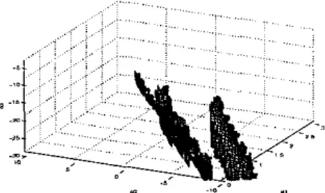
a z F ( u ) ) go to step 2.a.

Example 1. Consider determining proper first-order controllers to stabilize the plant go(s) =

$$

given in [l], where qo(s) = s5

+

3 s 4

+

29s3

+

15s' - 3s

+

60 and p o ( s ) = s3 - 6s'

+

2s

+

1. Algorithm 2 outputs the set of stabilizing ( a l , a ~ , a 3 ) values as shown in Figure 1.

Figure 1: Stabilizing set of (a~,az,as) values

4 Conclusions

In this paper a solution is given t o the problem of deter- mining all first-order controllers that stabilize a given plant. The method consists of an application of con- stant stabilizing gain characterization on two auxiliary plants.

An

extension of this method to any fixed or-

der controller is reported in [5] and to interval plants is reported in 141.

References

[I] Datts, A.. Ho. M. T. and S. P. Bhattacharyya, Strvcture and

Synthesrs of PID controllers, New York: Springer-Verlag, 2000.

[Z] Munro, N. and M. T. SBylemez, "Fast cornputstion of stabi- lizing PID controllers for uncertain parameter systems", Proc. QTd

IFAC ROCOND, Czech Republic, 2000.

[3] O z g d e r , A. B. and A. A. K q a n , " A n anaiytic determina- tion of stabilizing feedback gains", Report, Institut fur Dynamische Systeme, Report no. 321, Universitit Bremen, 1994.

[4] Saadaoui, k. and A . B. Ozgirler, "Computation of stabilizing first-order controllers for interval plants", Proc. 2"d International Conference on Signala, Svstems, Decision and Information Tech-

nology, Tunisia, 2003.

151 Saadaoui, k. and A. H. Ozgoier, " A new method for the computation of all stabilizing controllers of a given order", Technical

Report, Bilkent University, 2003.

Proceedings of the American Control Conference