Optimal replacement policies with minimal repair and random cost

POÎİCÎ4S 'JMfï

OPTIMAL REPLACEMENT POLICIES WITH

MINIMAL REPAIR AND RANDOM COST

A THESIS

SUBMITTED TO THE DEPARTMENT OF INDUSTRIAL ENGINEERING

AND THE INSTITUTE OF ENGINEERING AND SCIENCES OF BILKENT UNIVERSITY

IN PARTIAL FULFILLMENT OF THE REQUIREMENTS FOR THE DEGREE OF

MASTER OF SCIENCE

By

Hakan Levent Demirel

June, 1993

t i

Ί Θ ζ

I certify that I have read this thesis and that in my opinion it is fully adequate, in scope and in quality, as a thesis for the degree of Master of Science.

urler(Principal Advisor)

I certify that I have read this thesis and that in my opinion it is fully adecjuate, in scope and in (¡uality, as a thesis for the degree of Master of Science.

Professor Doctor Halim Dogrusoz

I certify that I have read this thesis and that in my opinion it is fully adequate, in scope and in quality, as a thesis for the degree of Master of Science.

Associs-te-ft'oTesso^.-B^tor Cemal Dinçer

Ap])roved for the Institute of Engineering and Sciences:

Professor Doctor M e h n i^ ^ ara y

ABSTRACT

OPTIMAL REPLACEMENT POLICIES WITH MINIMAL

REPAIR AND RANDOM COST

Hakan Levent Deinirel

M.S. in Industrial Engineering

Supervisor: Dr. Ülkü Gürler

June, 1993

When a system fails usually two actions take place; either replacement of system with a brand new one or repairing it if possible. In this study, it is assumed that system under consideration is repairable and is minimally repaired at failures with a random repair cost. Two replacement models are provided under this set-up. First model assumes that the system is replaced when the total cost of minimal repairs exceeds a total cost limit. Second model incorporates the number of failures into replacement decision. Here the concept of critical failure is introduced and used by means of two sub-models. In the first sub-model it is assumed that the system is replaced at the kth critical failure or at cige T. And the second sub-model assumes that the system is replaced at the first critical failure occurs after age T.

The first model is just constructed but cannot be solved due to complexity of the resultant function. But, solution methods of the sub-models of second model are provided.

Key words: Replacement Policies, Minimal Repair, Cost Limit.

ÖZET

DEĞİŞKEN ONARIM MALİYETLİ VE ASGARİ ONARIMIN

YAPILDIĞI SİSTEMLERDE DEĞİŞTİRME MODELLERİ

Hakan Levent Deniirel

Endüstri Mühendisliği Bölümü Yüksek Lisans

Tez Yöneticisi; Dr. Ülkü Gürler

Haziran, 1993

Sistemlerde meydana gelen bozulmalar genelde tamamen değiştirme veya eğer mümkünse onarma yoluyla giderilir. Bu çalışmada onarılması mümkün olan sistemler ve onarımin sistemi tekrar çalıştırmaya yetecek en küçük düzeyde yapıldığı varsayılmıştır. Bu doğrultuda iki değiştirme modeli sunulmuştur. Bir­ inci modelde sistem onarım maliyetlerinin toplamı hesaplanan maliyet limitini aştığında yenileniyor. Bu modelde amaç, maliyet limitini bulmaktır, ikinci model sistemde meydana gelen bozulma sayılanında dikkate alacak şekilde kurulmuştur ve iki ayrı değiştirme politikası içermektedir. Bu polikalardaki ortak amaç sistemin değiştirilmesini gerektiren onarım sayısını ve/veya yaşı bulmaktır.

Birinci model, ancak kurulabilmiş, sonuçta çıkan fonksiyonların kompleks olamsı nedeniyle çözüm önerisi getirilememiştir. Fakat ikinci model için çözüm metodları sunulabilmiştir.

Anahtar sözcükler. Bakım Onarım Sistemleri, Değişken Onarım Maliyeti,

Asgari (Minimal) Onarım

ACKNOWLEDGEMENT

I am indebted to Doctor Ülkü Gürler for her supervision, suggestions, pa­ tience and understanding throughout this thesis study. I am thankful to Asso­ ciate Professor Doctor Halim Doğrusöz and Associate Professor Doctor Cemal Dinçer for their interest in my thesis.

I would like to extend my deepest gratitude, love and thanks to my parents Nursel-Ozcan, my wife Didem and my brother Okan for their morale support and encouragement.

I really wish to express my sincere thanks to my friends Hakan Ozaktaş, Erkan Uçar, Murat Timur and Ihsan Durusoy for their precious friendship. And special thanks to Levent Kandiller, Vedat Verter, Nurettin Kırkkavak, Fatih Yılmaz, Selçuk Avcı and Fulya Abla for their guidance and support.

C ontents

1 IN T R O D U C T IO N 1

1.1 Reliability and Maintenance Policies 2

1.2 The Literature Review g

2 O P T IM A L R E P L A C E M E N T POLICIES 12

2.1 Replacement Based on Total Cost Limit with Random Minimal Repair C o s t ... 12 2.2 Replacement Based on Number of Failures and Age with Ran­

dom Minimal Repair Cost 19

2.2.1 Model A ... 21 2.2.2 Model B ... 35 3 CO N C LU SIO N 40 A Proof of Lemma 1 43 B P ro o f of W { k + [ , T ) - W { k , T) > 0 45 Vll

List o f Figures

2.1 Cost Limit P o lic y ... I4 2.2 Age Replacement vs Model A Policy I 28 2.3 Behavior of W{k^T) when k ^ 0 0... 32

3.1 Comparison of the three policies... 42

List o f Tables

'2.1 Example of Model A Policy 1 2.2 Age Replacement Model 2.3 Example of Model A Policy II 2.4 Example of Model B 27 33 38 2() IX

C hapter 1

IN T R O D U C T IO N

Due to developments in teclinology, new complex machinery and equipment are gradually replacing the labor force in manufacturing. Researches are being conducted both in industry and in universities to built factories of future where most of the operations are performed solely by machines. Such a development leads to factories that can be operated by fewer number of workers whose job are basically to control the processes. Since the percentage of machinery and equipment cost increases, as the labor cost decreases, they have to be used more effectively, efficiently and less costly. Studies such as machine scheduling, ])roduction i^lanning and control, inventory control, and material handling are conducted for effective, efficient and less costly manufacturing. Most of these studies assume that machinery or equipment for manufacturing are available whenever need arises. In reality however, this may not be true since breakdown of any machinery or equipment at any time is possible. Dealing with such possibilities pointed out the importance of maintenance planning. In this study, maintenance planning is examined under manufacturing environment, however the results are applicable to the other areas of interest including military, hecdth and fire services, railroads, highways, so on.

For a typical manufacturing plant, the importance of maintenance planning comes from the consideration of the following questions;

• VVh<at, is the true, practical life of the components that are critical to the machines that convert raw materials to finished goods? When is the right time to replace parts?

• How much money should be budgeted for maintaining the plant’s infra­ structure? When should the expenditures be made?

• What is the lifetime for the major pieces of manufacturing equipment? When should new machinery become the alternative decision?

• How do you ensure that a critical machine is not disabled at the moment of need?

• How much of the maintenance cost should be allocated for emergency repair, preventive maintenance, predictive maintenance or normal repairs?

• What is the management’s role in the maintenance system?

In this study emphasis is put on the optimal replacement of systems subject to stochastic failures. It is hard to place this problem as an answer to any of the above questions, but as can be seen it is common for most of them.

In a manufacturing environment, a machine, a production line, a manufac- turing cell, a material handling system can be considered as a system. Missiles, tanks, aircraft can be considered in military environment. Ambulances, x-ray equipment, surgery room can be considered for health services. No m atter which environment is under consideration, the main point is to decide when to replace the system to ensure that they are used effectively, efficiently and less costly, and they are availal/le whenever need arises.

CHAPTER I. INTRODUCTION 2

1.1

R e lia b ilit y a n d M a in te n a n c e P o lic ie s

The study of maintenance policies is a part of Reliability Theory and involves a broad range of decision-making problems. Some of them are Replacement,

CHAPTER. 1. INTRODUCTION

Repair, Inspection, Repairman Problem, Spare Parts Inventory, and Number and Allocation of Standby Units. Before going into the description and the scope of these decision-making problems,some concepts of Reliability Theory will be introduced first.

Reliability theory is concerned with determining the probability that a sys­ tem, possibly consisting of many components, will function during the mission time. For instance, a series system will function if and only if all of its com­ ponents are functioning, while a parallel system will function if and only if at least one of its components is functioning.

During the mission time of a system there may occur some undesirable events due to environmental or internal conditions. These undesirable events, so called failures, cause disru])tions in the process. A failure is the result of a joint action of many unpredictable random processes going on inside the operating system as well as in the environment in which the system is operating.

Replacement policies incorporate the studies about the stochastic nature of the failures of the system with optimization methods to achieve a desired amount of quality. By cpiality, a quantitative measure such as, system reliabil­ ity, system availability or cost of maintenance is meant. System reliability and

system availability are defined in terms of the lifetime of a system.

Lifetime of a system is the random time from the beginning of the operation

until the appearance of a failure and it is the source of the uncertainty in maintenance decision making. Lifetime highly depends upon the structure of a system. For a singhi-unit .system (can be considered as a part of a whole, as well) lifetime can be determined without having complex analysis, but for a multi-unit system lifetime is a function of lifetimes of units that built the system.

Let A’ be the random variable denoting the lifetime of the system. Then

V { X > Xo), which is the probability that X exceeds a value Xq., is the system reliability (or the sxirvival probability) for a mission time of ;Co· P {X > x) — 1 — F{x) is called the survival function with F{x) being the cumulative distribution

CHAPTER. 1. INTRODUCTION

function of the random lifetime X.

System, availnhility is the probability that for a specified period of time the

system is available for operation. There are several availability measures as defined below;

i) Point avnilnhility is the probability that at a given time instant, say t, the system is available for operation, i.e. let I{t) = 1 if the system is operational at time t, 0 otherwise. Then, point availability, A{t) is defined as = V[I{t) = 1].

ii) Lim.iting availability; is the expected fraction of time in the long run over which the system operates, i.e.. Limiting availability (/1) = limt_oo A{t) if the limit exists.

Other forms of availability such as interval and limiting interval avaihibility are also used to express quantities of interest for maintenance decision-making.

Failure rate (or hazard rate) r[t), and Cumulative failure rate R{t), play

key roles in maintenance decision-making. Failure rate of an equipment at time t is proportional to the probability that the equipment will fail in the next small interval of time given thcit it is good at the start of the interval. Let

F{t) be the distribution function of the lifetime variable X, and suppose the

density function f{t) exists. Then the failure rate r{t) is defined as.

?■(() m 1 - F(i) (1.1) Note that. r(t) = lim — VU < a; < /, -f A t\x > t) ’ Ai-O A t ’ = lim Ai—0 F ( t T A t ) - F ( t ) At F( t ) (1.2)

If Fft) does not possess a density, i.e. if it has discontinuities, analogous definitions of the failure rate also exist. However throughout this study, it

CHAPTER I. INTRODUCTION

is assumed that F{t) is absolutely continuous and the density exists. If

r{t) given in (1.1) is increasing with t, then Lifetime distribution F{t) is an

increasing failure rate (IFR) distribution. Conversely, it is a decreasing failure rate (DFR) distribution if r(i) is decreasing with t.

The cumulative failure rate R{t) is defined as R{t) = fQr(t)dt. The survival probability can be expres.sed in terms of cumulative hazard rate as F(f.) =

p - m

After introducing some concepts of reliability theory, what follows in the sequel is the description and scope of maintenance decision making problems.

R e p la c e m e n t: Replacement decision making involves determining the time of replacement of a system under some optimization criteria, such ¿is; minimizing total cost, maximizing availability, etc.

Usually two types of policies are considered for the replacement decisions: age replacement and block replacement. Under age replacement^ the system is replaced upon failure or at age T, whichever comes first. Usually, ci is assumed to be the cost of reidacement at failure and 02 is assumed to be cost of replacement at age T, where Ci > 02. For age replacement, the average

long-run cost per unit time is given by;

c,F{T) + C2F{T)

C{T) =

lo m d f · (1.3)

Under block (periodic) replacement the system is replaced upon failure and at times T, 2T, 3T · · ·. The expected cost per unit of time following a block replacement policy at interval T over an infinite time span is given by;

Cl M{T) + 02

C( T) =

T (1.4)

where M{ T) is the expected number of failures in [0, r ) (renewal function) corresponding to the underlying lifetime distribution. For the derivation of above formulas refer to [5].

R e p a ir: For repairable systems, two types of repair have been considered; minimal and imperfect rej)air. Minimal repair concept was first introduced by

Barlow&Hunter [3]. Under minimal repair, it is assumed that the repair ac­ tion returns the system into operational state but system characteristics are the same as just before failure i.e. the system is as good as old. In other words, sys­ tem ’s failure rate remains undisturbed by any repair of failures. Minimal repair is an appropriate model for complex systems such as computers, airplanes and large motors, where system failure occurs due to com])onent failure and sys­ tem can be made operational by replacing the failed component by a new one. Therefore the system characteristics are nearly the same before and after fail­ ure. Formally, minimal repair can be defined as follows [23]: Let Vj, · · ·, V],, · · · denote the successive failure times of a system and X,i — Y,i — T,i_t be the time between failures, where Vq = 0. Let F{t) = V{ X\ < t), then the system undergoes minimal repair at failures if and only if

r{X ,i < X |Al + A'2 + · · · -f A,i_i — t) — ---;----7=rrr\---- ~

CHAFTER I. INTRODUCTION G

l - C ( l ) for X > 0, t > Q.

Right hand side of the above equality is proportional to the failure rate given in ( 1.2), so the equality states that system failure rate remains undisturbed by any minimal repair of failures.

Let Nt be the number of failures in [0,f) for a system which is subjected to minimal i-epair after each failure. Then the distribution of Nt follows a non- stationary Poisson Process with an intensity function r(i), where r{t) is the failure rate of the lifetime variable. Moreover, expected number of failures in [0, i) is = R{f.) (see [20] and [3]). Then,

Vi Nt = n) = -^(‘)[R(0 ]'‘ (1.5)

The concept of imperfect repair has originated from the discussion about

imperfect maintenance which has appeared in [25], [24], [21] and[7]. In these

studies, it is argued that, due to repairing the wrong part or only partially repairing the faulty j)art or while repairing the faulty part damaging some adjacent parts, the maintenance action may not be as perfect as it is assumed to

CHAPTER 1. INTRODUCTION

be. Thus, maintenance action is divided into two categories in terms of repair. The system may be a.s good as new after a perfect repair, or it may be as good as old after a minimal repair. Brown and Proschan [6] put the framework of the imperfect repair and provided useful results. According to their discussion, under imperfect repair, a system is repaired at failure. With probability p it is returned to the as good as new state (perfect repair), with probability {[ —p) it is returned to the functioning state as good as old (niinivial repair). Imperfect repair is the generalization of minimal repair since an imperfect repair with p = 0 is a minimal repair.

In sp e c tio n : The basic purpose behind an inspection is to determine the state of the equipment. The indicators, such as bearing wear, gauge readings, quality of product, etc. which are used to describe the state, are specified. Then the necessary maintenance actions are taken accordingly. .An inspec­ tion schedule must balance the trade-off between cost of inspection versus the benefit of correcting minor defects before major breakdown occurs.

S p a re P a rts In v en to ry : Usually, when a replacement decision is made, it is assumed that the system or some of its parts which are subject to re­ placement are available whenever they are needed. But, keeping everything on hand is both expensive and at some instances not possible. So, optimal level of inventories and for which units these inventories will be kept must be determined. This area of interest is newly considered in the literature due to developments in solutions to inventory problems.

S ta n d b y U n its: Several number of standby units are placed on to the sys­ tem so that whenever a unit is failed it is replaced by its standby immediately. The research problems in this area are related to finding the optimal number of standby units to be placed for fulfilling an objective (e.g. minimizing cost or maximizing availability). Allocation of standby units, i.e. for which units they should be u.sed, is another consideration.

The decision-making issues mentioned above are not independent of each other. Usually two or more of them are taken into account for a maintenance policy. For example; a system may be inspected at fixed points in time together

with being re|)<iirecl at failures and can finally be replaced when its cost of operation exceeds or reliability level reduces below a certain permissible level. The aim of such a policy may be to decide the frecpiency of inspections, how to repair and when to replace the system in order to utilize the system more effectively, efficiently and reliably.

1.2

T h e L ite r a tu r e R e v ie w

CHAPTEfi 1. INTRO DUCT ION 8

In the past three decades, many scholars and prcictitioners have shown inter­ est in the study of maintenance models for the systems with stochastic failure. One major reason for this is the fact that maintenance models have various ap­ plication a.reas such as military, industry, health and environment. As systems become more complicated and recpiire new technologies and methodologies, more sophisticated maintenance models and control policies are needed for their effective usage.

One of the main references about maintenance models is the book by Barlow&Proschan [5]. Later, several others followed, including Barlow and Proschan [4], Certsbakh [L3] and .Jardine [16]. In addition, several survey pa­ pers have been published in this area, including Cho and Parlar [8], Thomas [.32] and Pierskall and Voelker [27].

In the sequel, studies about several maintenance models are provided. Most of them are related to the replacement of a system under different conditions. Studies related to other maintenance actions are also provided briefly.

Kaio and Osaki [18] reviewed some discrete and continuous lifetime dis­ tributions and ap])liecl them to typical rephicement models of age and block rephicement. They [provide the resvdt in tables as a reference guide.

Derman et.al [11] considered an extreme version of the replacement prob­ lem. Under their model, a vital component of a system must be replaced before

CHAPTER 1. INTRODUCTION

it fails, otherwise the system fails with no possibility of repairing. They as­ sumed n spare units and their objective is to maximize the expected life of the system.

Mehrez and Stulman [19] modifies the age replacement policy by introduc­ ing inventory constraint. They argued that instantaneous replacement is not always possible due to lack of spare units so that they have provided an age replacement model constrained by two inventory models.

Flynn et.al [12] studied a multi-component system and they based their policy to CCP (critical component policy) concept. This is similar to CPM (Critical Path Method) in project management. Their objective is to find the replacement policy of comi)onents which minimizes the long-run average cost per period. They showed that it is optimal to replace a failed component if it is a critical one.

Nakagawa and Kowada [23] aiuilyzed a system with minimal repair at fail­ ures. They provided the formal definition of minimal repair, and derived some probability and reliability quantities. They had applied their result to a re­ placement policy. In particular, they assumed that system under consideration is subject to minimal repair at failures and is replaced at a prespecified age T or at the nth failure, whichever occurs first. They provided the conditions under which the optimal number of failures is finite cind unique. Their work did not assume random repair cost. A Similar work has been carried out by Nguyen and Murthy [26], but they assumed that after each repair the failure rate is increased. They considered two policies based on this assumption. Policy I is suited for single unit systems and Policy II is suited for multi-unit systems.

Hayre [14] provides a study about deciding whether to repair or to replace. He assumed a system which deteriorates over time. When the deterioration reaches a critical level, the system has to be either repaired or replaced by a new one. Repairs are cheap but usually less effective so that new failures might occur shortly after repair. Replacement is costly but it renews the system. He modeled this trade-off between repair or replacement as a semi-Markov decision process and minimized the long-run average cost ]>er unit time. Similar to this

CHAPTER 1. INTRODUCTION 10

study, Yuii and Bai [03] considered a repair cost limit policy for a system with imperfect repair. Their aim is to find an optimal cost limit L over an infinite time horizon, which is vrsed for the decision of repair or replace at fiiilures. They assumed that repair cost is a random variable and if the estimated cost of repair is beyond the value of T, it is economical to replace the system. They found an expression for the expected cost rate with respect to repair cost and cumulative hazard function. Because of the difficulty of the analysis of the expression for general failure distributions they used a Weibull failure distribution and a negative exponential distribution for repair cost. They showed that under these distributions, value of L is finite and unique. On their earlier study, Yun&Bai [2] considered the same model for a system with minimal repair at failures. Under this model the system is repfivced either if the estimated cost of minimal rejiair on a given failure exceeds a calculated cost limit value L or at age T, whichever occurs first.

Cleroux et. al. [9] consider the age replacement policy with minimal repair and random repair costs. They assume that replacement of the unit at the failure is depend upon the random cost C of repair. Under their policy a replacement at failure takes ])lace if C > Sci, where Ci is the constant cost of replacement at failure and 6 is a given percentage of the cost Ci. The variable 6 is assumed to be a known parameter by the decision maker. They had provided the cost function over an infinite time span and the solution algorithm for finding the optimal planned replacement times.

In this study, the cost limit policy of Yun and Bai [2] is modified to con­ sider a total cost limit. In particular, the optimal total cost limit, L, is inves­ tigated if the system is replaced when the cumulative cost of minimal repairs exceeds L. When the costs of minimal repairs are assumed to be independently and identically distributed continuous random variables, the long-run aver­ age cost function, obtained by the Renewal Reward Theorem, becomes quite intractable. Neverthele.ss, average cost function is derived and presented in section 2.2. Since average cost function becomes highly complex for a general continuous minimal repair cost distribution, a sj)ecial discrete cost model is considered in section 2.3. Under this special cost distribution, replacement

CHAPTER 1. INTRODUCTION

models considering the number of failures are studied.

For all of the models that are considered in the present study, the long run average cost per unit time function is analyzed. From Renewal Reward Theorem (.see Ross,f28j), this long run per unit time cost can be obtained by dividing the expected total cost in a replacement cycle to the expected length of that cycle. Let C be the average long run cost per unit time, then

C ¿[total co.si]

¿[length] (1.6)

Notation

Several notations are used throughout the study, those of which are common to all policies are listed below. Model specific notations are provided in their related sections.

/(¿), F(f), F{t) pdf, Cdf, Sf of the system’s life time.

7‘(f), R{t) failure rate and cumulative failure rate of the system.

Nt number of failures in [0,i).

X{.) indicator function which returns value 1 if the argument inside the parenthesis is true.

¿{.) Expected value of a random variable. T ’ optimal replacement age of the system.

cr cost of replacement of the system with a brand new one.

Assumptions

1. The planning horizon is infinite.

2. Repair and replacement times are negligible.

3. r[t) is strictly increasing and remains the same after each failure. 4. Lifetime distribution F[t) is continuous and its density f{t) exists. 5. Time value of money is ignored.

C hapter 2

O PT IM A L R E P L A C E M E N T

PO LICIES

2.1

R e p la c e m e n t B a s e d o n T o ta l C o st L im it

w ith R a n d o m M in im a l R e p a ir C o st

In their study, Yun and Bai [2] consider a system subjected to failures for which minimal repair is performed. Under their assumption minimal repair cost is a random variable. Their aim is to find a cost limit L over ¿in infinite time horizon such that, if the estimated cost of a repair at a failure exceeds the calculated value L, the system is replaced. Their policy is to continue to repair the system as long as the estimated cost for each failure is below L, replace it if the cost of a repair is more than L or at the first failure that occurs after age T, whichever occurs first. Such a policy gives a comparison value to the decision maker in order to decide whether to repair or replace the system at the time of failure.

In the present study, Yun and Bai’s cost limit policy is modified to incor­ porate total cost limit. In other words, rather than finding a cost limit to compare repair costs, a total cost limit is investigated to compare cumulative

CHAPTER 2, OPTIMAL REPLACEMENT POLICIES

repair costs. Policy under total cost limit is to continue to repair the system while the sum of the re|)air costs are below a total cost limit, L, and replace it when the total cost limit exceeds L.

Notation and Assumptions

X.

v;

L'

pdf and Cdf of the repair cost .

r?,-fold convolution of G'(x), gix) respectively.

cost of minimal repair of /ith failure having distribution function of G{x)

time of the ¿th failure. optimal total cost limit.

number of failures before the total repair cost e.xceeds L.

1. Repair cost distribution G{x) is continuous and its density g{x) exists 2. Xi's are independent and identically distributed.

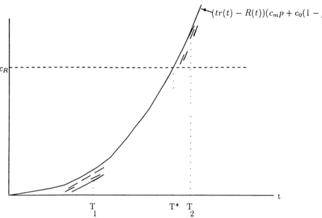
The system under consideration is minimally repaired at each failure with a random repair cost of A’i, i = 1, 2,··· and when the total repair cost exceeds a calculated cost value, L, it is replaced with a brand new one. X{, i = 1, 2, · · ·, are distributed by G(.'r), :re(0,oo), where Xq — 0. Let Yi be the time of the ith

failure, then V] ~ F{f.)

In Figure 2. 1, a typical behavior of the system is shown. Since at the 4th failure total rej^air cost (A’l + X^ + .A3) exceeds L, the system is replaced.

Let S,i sum of minimal repair costs of n failures, then

t=l Define

CHAPTER 2. OPTIMAL REPLACEMENT POLICIES 14

C(L)

A'3

V', >3 >4

CHAPTEfi 2. OPTIMAL REPLACEMENT POLICIES 15

where is the nuiiil)er of failures before the total cost of repair exceeds the total cost limit L.

• Expected total cost until replacement : The total cost incurred by the replacement time is given by from the results of renewal theory. Then expected total cost of a replacement cycle is given as,

S[Total = o[.S'n^] + cr

From Renewal Theory, the survival function of is,

V[Sn, > .s) = G{L) - r G[L - y)dM{y) f or ,s < L Jo where M{s) = ^ ' ”=1 GG){s) and P (5„ < s) = GG){s). Thus,

£1%,]

=

r

Adding the cost of replacement to the above equation leads,

:2.2)

(2.3)

(2.4)

S[Total Cost\ = ca + LG{L) - £ - y)G[L - y)y^"-\y)dy (2.5) u=l

^0 •

• Expected length of a replacement cycle : Since is the time of the ¿th failure, V'kt+i is the time of the failure where replacement occurs so that it is the length of a replacennuit cycle. Then the expected length of a replacement cycle, found by conditioning the expected length to the number of failures;

CHAPTER 2. OPTIMAL REPLACEMENT POLICIES 1()

- X) + 1 = n) (2.6)

n = l

V{'^1 = n) in (2.6) is the probability that, at the nth failure the total repair

cost is below L, and at the (n + l)st failure, total cost exceeds L. Then,

= n) = V{Xi + · · · + AT < L, AT + · · · + AT+, > L) T’iAi + · · · + A,I ^ L) — T[ Xi + · · · + > L)

= 6'<'6(L) - (2.7)

So, (2.6) can be rewritten as.

= E = n](G(’0(^ ) _ G’("+i)(L ))

71=1

In order to calculate = n], 7^(V„+i > t) must be determined. Note thiit,

V{Yn+i > t) = V{Nt < n)

and V{Nt = n) is already stated in (1.5). Hence,

t = l 'll

Then,

T[VH.+,|K = n ] = r z

.=0 (It

Finally, combining (2.9) and (2.8) yields.

/*00 ‘ = E ( C '''”>(i) - G'"+'>(i)) / E

n=l i=0

12.9)

CHAPTER 2. OPTIMAL REPLACEMENT POLiCIES

The above equation can be simplified by changing the order of summations;

- ..x>

Sllength] =

1=0

^

^

-(It

(2.11)

As a result, from (2.5) and (2.11), the average cost per unit time function of a system subject to minimal repair at each failure and which is replaced when the total cost limit is exceeded is given ¿is follows;

C ( i ) = LG(L) - E ” I /»''(G - y)G[L - y)</''Kv)d,j + c„

Jo” «-*'''«(')'■<«

(2.12)

The above equation is so hard to analyze for a general cost distribution due to convolutions. Even if the cost distribution is selected to be exponential (where n-fold convolution of exp(A) is r(n,A )) the above function is still in­ tractable. Due to this rea.son similar models will be studied in the next .sections. This section is ended with the following analysis: let,

rm

then,

Z (i) = / z (t, x)/y"'^(x)(Ix

Jo

zi(t) =

Using the above relation, and setting the derivative of (2.12) to zero yields the following relation:

W(L)[G(L) + Lg{L) - f ; i ‘'[-yG(L· - ;;) + ( i - g)glL - y)V/"\y)dg\ 11=1 oo ¡.L -L G [L ) - Y , ( L - y)G{L - ¡/)a"‘l(!/)<i!/ = c„ 1

Jo

CHAPTER 2. OPTIMAL REPLACEMENT POLICIES 18

The value of L which satisfies the cibove equation is a candidate for an

optimum L. However providing results for the existence and uniqueness of L

CHA PTER 2. OPTIMA L REP LA CEMENT POLICIES 19

2 .2

R e p la c e m e n t B a s e d on N u m b e r o f F a il­

u r e s a n d A g e w ith R a n d o m M in im a l R e ­

p a ir C o st

In the previous model, the difficulty of dealing with minimal repair costs having general distribution functions was pointed out. In this iiiodeb a special discrete minimal repair cost distribution is introduced and used under different policies.

During the operation of a system several number of failures may occur. The repair cost of each failure varies according to the nature of the failure. For instance, a resistance failure in the power card of a computer stops the operation, but the computer can be operated by replacing the resistance with a small cost. On the other hand, if the whole power card of the computer was burn out, then a considerable amount of money must be paid to bring the computer l)ack to operation. Suppose failures are divided into two categories in terms of cost. Some failures are more expensive to recover (e.g. power card example), call these critical failures, whereas some require considerably less payment (e.g. resistance example), call these non-critical failures. Such a distinction lead to a discrete repair cost distribution function defined as follows;

Let Xi be the cost of /th failure, i = 1, 2, · · ·. Suppose that with probability the failure is criticcil and the cost is c„i, and with probability (1 — /;) it is a non-critical failure which costs Cq. So, for each

Cjn with probability p Co loith probability (1 — /;)

(2.13)

With the al)()ve cost t’linctioii, two replacement models are considered. In the first model the system is minimally repaired at failures and replaced when k critical failures occur or at age T, whichever occurs first. In the second model, the system is minimally repaired at failures and replaced at the first critical failure occurs after time T.

CHA PTER 2. OPTIMA L REP LA CEMENT POLICIES 20

thus it is possible to find V{N^ = k) by conditioning on total number of failures.

ViN^ = A.·) = £ V{Nt = n)V{N^ = k\Nt = n) l = k

Since with probability p, a failure is a critical one;

v{N^ = k) =

Notation P Fy{t.) N1^ AVf X.

v;

probability that a failure is a critical one,

{(I-p) probability that a failure is non- critical),

distribution of time between critical failures, number of non-c.ritical failures in [0,A). number of critical failures in [0, t).

random cost of fth failure defined in (2.13). time of the /th critical failure,

optimal number of critical failures to replacement, optimal age of the system for replacement,

CHAPTER 2. OPTIMAL REPLACEMENT POLICIES 21

cost of repairing a critical failure It is obvious tliat Cq < c„i < <'r

2.2.1

M o d el A

In this model, tlie system under consideration is replaced at the time of kth critical failure or its age T, whichever occurs first.

Firstly, the cost function which represents tlie long-run average nuiintenance cost per unit time will he constructed. As stated before, it is composed of two expressions: Expected length and expected total cost.

• Expected length of the replacement cycle : There exists two possibilities for the length of the replacement cycle, it can either be age T if less than k critical failures occur in [0,T], or the time of the kth critical failure if it occurs before T. Let RC denote the length of the rei)lacement cycle, then,

RC = TI { Yl > T ) + < T) (2.19) and,

€[RC] = S [ T I { Y , > T ) + £ [ Y k I { y i < T )

= TViYk > T) +

r

Jo

To evaluate 7^(V'i· < T), note that V{yi- < t) = T’(iV)·' > k). From (2.L5), e“'’^(d[p/?(i)]^· iP(yV)· = k) = k\ So,

v{N^>k) = 5:

CHAPTER 2. OPTIMAL REPLACEMENT POLICIES ·)·}

Let Hk{t) = V{Yk < t), then

« ,( / ) = 1 - 5 : (2.22)

j=0 So, going back to €[RCY

T

£[RC] = T H k( T ) + f ijdlhiv) (••^•••^3)

Jo

Applying integration by parts to the integral in the above equation yields;

£\RC] = f

Jo Hk{y)di (2.24)

• Expected cost until replacement: Maintenance co.st is the result of two types of repairs, tho.se for critical failures and those for non-critical failures. Thus, by using (2.17) and (2.18), expected cost until replacement can be found.

For the number of failures, two possibilities exist: system may be replaced at the time of A:th critical failure, so that there are k critical failures and Ny^ non-critical failures; or the system may be rejilaced at its age T so that Ny critical; and Ny non-critical failures occur. Let N F stand for the number of failures, within a replacement cycle, then;

N F = [k + N i n i i Y k < T) T [Nly -t- 7V^]J(y', > T) (2.2,5)

Taking the expectation of both sides of (2.25);

S[NF] = £[[k + N{{]I{Yk<T)] + £[[N^- + N ^ ] I { Y k > T ) ] (2.26) = k V { Y k < T ) + £ [ N l I { Y k < T ) ]

+£[N!jJ{Yk > T)] + £ m i { Y k > T)]

First note that;

I(V i < 7’)] £[£[Nll{Y„ < T)\Yt = ¡11 J I ( ¡ < 7)1

í ( ( ı - r t f i ( ¡ ) I ( ¡ < г ) l

CHAPTER 2. OPTIMAL REPLACEMENT POLiCiES 23 also, > T )] = _{S[N:rI{Nr < f^)]} ^ .e - ’>^^T'[pR{T)Y = ---¿=0 pR (T )f l,_ ,{ T ) ¿• = •2.3, 0 k = \ . C2.-28) Next, £ [ N ^ I { y i > T ) ] = £ m r { Y , > T ) = { l - p ) R { T ) f h { T } (2.29)

Finally, from (2.27), (2.28), (2.29), and introducing the costs;

£lfaHure CO.R.] = c,nlkH,(T) + pR(T)H,_i(T)]

C o ( l - p ) l/ ^ R(t)dH,(i) + R ( T ) H ,( T ) (2.30)

Thus, expected total cost until replacement, from (2.30) and adding re­ placement cost of Cft, is;

£[iotal co.^t] = c, 4kLR(T)+pR(T)/ 7, _i(T)j (•2.31) +co(l - p)[J^^ R ( i) d f R ( n + R(T)H,(T)j + CH

Let Cfc(T) be the long-run average cost per unit time of a system subject to replacement either at ktdi failure or at age T, then from (2.24) and (2.32);

c„ikHt{T) + pR{T)Ht-,(T)] + co(l - p ) l g Hult)dFi(t)] + cr

Ct(T) =

¡ ¡ I h i t

(2,32) The above function of Ck{T) is analyzed under two policies given in the fol­ lowing .sections.

CHAPTER 2. OPTIMAL REPLACEMENT POLICIES 24

Policy I.

Under some circumstances the number of critical failures that the system man­ ager is willing to allow before replacement can be prespecilied. Then the only concern is to find a replacement age T* which minimizes the cost The reason why only the critical failures are considered for replacement decision is that each critical failure adds more cost to the total cost figure than non-critical failures in a given replacement cycle.

Assuming that k - ko, (2.32) can be rewritten as follows;

U^-okh,{T) + pR.{T)fh,^,{r)] + co(l - p) f h J t ) d R { t ) + cn ) =

---(2.33) The following lemma will be necessary for the proof of the Theorem 2.1 Lemma 1 : Let

■'hAT) = .-(D li'^p + cCi - /,) ! - C i j T )

i) i/jicoiT) is increasing in T € (0,oo). ii) LimT_^ikf;^{T) = (X) if F{t) has IFR.

Proof : Provided in Appendix.

Theorem 2.1 i) Optimal replacement age T* which mvnwiizts (2.3o) is the value of T which satisjics;

r(T)[c.„,, + c „H -p )] = C tA r) (2„34)

a) If there exists a T* then it is unique f o r T G (0,(X)).

hi) If no solution to (2.3/^) exists then a policy of replacement only at koth failure is optimal.

CHAPTER 2. OPTIMAL REPLACEMENT POLICIES 25

P ro o f, i) Differentiating (2.33) with respect to T and equating to zero gives (2.34). Thus, optimal replacement age T* is the value of 7’which satisfies the equality in (2.34).

ii) For T = 0 fpkoi^) = —{koCm + cn) < 0 and from Lemma 1, iho{T) is increasing and tends to infinity as T —»· oo.

Thus, ipkoiT) starts from —cn, then cross zero, which meiuis a 7'* exists, and goes to infinity. Also it crosses zero only at once so that T* is unique.

iii) If no solution to (2.34) exist, then T" — oo, so that there is no need to consider the age of the system.

Example

In order to demonstrate the use of model, the case A:q = 1 will be analyzed.

In particular, the system under consideration will be replaced at the time of the first critical failure or age 7', whichever occurs first.

Cost function for k) = 1 is in the following form;

c,,Nh{T) + C o i l - p) ¡0^' Fh(t)dR{t) + cn CAT) =

¡A H u m

[(1 — e + Cq(1 — /;))] + cji

(2.35)

From Theorem 2.1 and Lemma 1 the value of T* which minimizes (2.35) can be found from

i(3 ’)[c'„.;' + <.'o(l-;))] =

C,(r)

The VVeibull distribution is selected for the lifetime variable. Probability density function of Weibull is: f{t) = and F{t) = 1 — e“ '". This distribution has IFR if « > 1. Also, /■(<) = aC '“ ' and /?(i) = C.

The optimal replacement age T “ which satisfies (2.36) can be found by numerical search. The integrals in the function is approximated by Trapezoidal

CHAPTER 2. OPTIMAL REPLACEMENT POLICIES 26

are divided into n suh-intervals by taking n = 7’/0 .000001 where T is the upper limit of the integral.

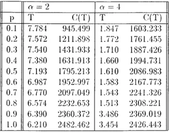
Table 2.1 summarizes the optimal replacement ages for two different shape parameters (a) under cq = 50, c,n = 200 and = 2000.

cv = 2 O' = 4 P T C(T) T C(T) 0.1 7.784 945.499 1.847 1603.233 0.2 7..572 1211.898 1.772 1761.455 0.3 7.540 1431.933 1.710 1887.426 0.4 7.380 1631.913 1.660 1994.731 0.5 7.193 1795.213 1.610 2086.983 0.6 6.987 1952.997 1.583 2167.773 0.7 6.770 2097.049 1.543 2241.326 0.8 6.574 2232.653 1.513 2308.221 0.9 6.390 2360.372 3.486 2369.019 1.0 6.210 2482.462 3.454 2426.443

Table 2.1: Example of Model A Policy I

The error bound for the integral (from page .206 of [31]) in the denominator of (2.35) due to trapezoidal approximation is about d.OObE — 7 given that /j = 0.1, and T* = 7.784 which is the optimal T of the first cost combination. Under both shape parameters o-, as the probability of critical failure occurrence increases, age T decreases while average cost is increasing.

When p = 1, Policy I is eriual to classical age replacement policy, because when p = 1 (2.35) is of the following form,

I i m - u

where F{T) = 1 — Then by adding and substracting crF{T) to the

numerator yields,

,, (c.,. + c«)f(J-) + c k'F(T)

irmt

CHAPTER 2. OPTIMAL REPLACEMENT POLICIES 21

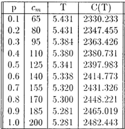
in (1.3), for Cl = c„i + Cfi. Thii.s comparison of the two policies; age replace­ ment and Policy I of Model A is possible by letting c,„ · ;;c„i + (1 — p)co i.e. considering the probability p as the weight of the cost of repair in expectation. For example, when = 0.1, c„i in age replacement cost function can be taken as c„, = (0.1)(200) + (0.9)(50) = 65.

Table 2.2 summarizes the optimal age values of age replacement under the listed c,n values for VVeibul^a = 2).

P T 0(T) 0.1 65 5.-4.31 2330.233 0.2 80 5.431 2347.455 0..3 95 5.384 2363.426 0.-4 n o 5.380 2380.731 0.5 125 5.341 2397.983 0.6 140 5.338 2414.773 0.7 155 5..320 2431.326 0.8 170 5.300 2448.221 0.9 185 5.281 2465.019 1.0 200 5.281 2482.443

Table 2.2; Age Replacement Model

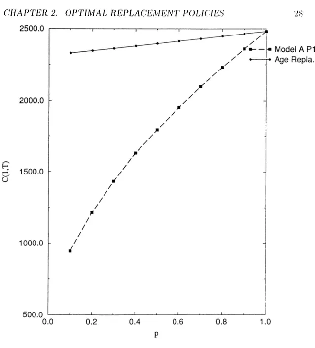
In Figure 2.2, long-run average cost per unit time for each p is given. As can be observed Policy I of model A gives better results as oppose to age replacement for this specific case. This leads to the discussion that, if it is possible to distinguish failures in terms of cost and find a probability p to be used in repair cost distribution, it would be beneficial to employ policy I rather than age replacement.

Note that Policy I is similar to total cost limit policy, given in the previous section, since the cost of critical failures is fixed to a limit of (koCm). However these policies are not identical, box'ause the decision is made by considering only one type of failure so that the contribution of the other type is not taken into account.

CHAPrEli 2. OPTIMAL REPLACEMENT POLICIES 28

Figure 2.2: Age Replacement vs Model A Policy I Policy II.

In the previous policy, optimal replacement age T ’ is analyzed when the num­ ber of critical failure's is s])ecified in advance. Under Policy II., the value of k", which minimizes (2.22) will be investigated, for a fi.xed T.

Suppose that, the number of critical repairs k is not considered for replace­ ment decision and the only concern is to determine the optimal T. Then the corres])onding cost function can be obtained by letting ^ > oo in Ck{T). The following lemma is needed for the analysis of C,yc.{T) = lim/;;_,x, Ck{T).

CHAPTER 2. OPTIMAL REPLACEMENT POLICIES 2!) Lemma 2 linu._oo I - i k i T ) - 0 linu-^oo Hk{T) = 1 HUt)dR{t) = R{T) lim,_oo fo H,{t)dt = T

Proof: Obvious from the sum of Poisson probabilities.

Now. from the above lemma,

c„ipR.{T) + co(l — p)R{T) + Cfi C .A T) =

(2.;37)

T (2.38)

If there e.xist a T ” which minimizes the above equation then it must be the root of the equation in the following implication;

dC^{T) dT = 0 (c„,p + Co(l - v))r{T) = C ^ { T ) or. Tr[T) - R{T) = Cr [CmP + Coi 1 - />)) (2.39) (2.40)

RHS of (2.39) is equal to the equation provided in (2.34) when k is selected to be oo. The following theorem gives the conditions for determining the optimal A;* for a fixed T.

Theorem 2.2 i) If l.here exist;> a T" which ftati-iificit (2.40), then for any T >

T* there, exists a finite mid unique k” which satisfies

\V{k-,T) > CR and W{ k' - l , T ) < Cr (2.41)

where

W(k, T) = t’ [(yc... + (1 - rtco )i/n .,(r)l

(2.42)

-CHAPTER 2. OPTIMAL REPLACEMENT POLICIES ;50

Note that W { k , T ) = 0 for A: = 0 a7id incrca-niuj with k.

ii) For any T < T*, no A* satisfying (2-41) exists. So reylaccinent should be at T = T*.

Hi) If 710 T* satisfyi7ig (2.40) exists, i.e. T* = oo, thcji /lo A* ca/i he found. Fmally, no solution to 7nai7ite7ia7ice problem exist.^.

Proof.

i) If any T > T* is selected for the replacement age then, to find a A’ which minimizes C{k ,T) following inequalities can be formed;

C { k ’ + 1,7') > C { k C T ) U 7 i d C { k \ T ) < C { k ' - 1,T )

Then, by examining C(A + 1, T) — C { k , T ) > 0 and C { k — 1, T) — C { k , T ) > 0, and letting LHS of the inequalities be W [ k , T ) yields (2.41).

The function W { k , T ) is increasing in A since W [ k + 1,T ) — W { k , T ) > 0 (proof is given in appendix). Now let

W{oo,T) = lim W { k , T )

then

VK(oo.T) = (Tr(T ) - R{T))(c,„p + co(l - p) (2.43)

This can be shown as follows; From Theo/rmi 3 of [23]

If (¡)[t) and i){t) are continuous functions and, <j){t) 0 and 0{t) ^ 0 then;

(2.44) / P V i o * m lim — f:tfi){i)dt i){b) Then, with f„{t) - pr{t)Ff’{T); .=A;+1 *·

CHAPTER 2. OPTIMAL REPLACEMENT POLICIES :|l

¿ii:i j T liiii i " " _{lo {pR{t))^}

Next, the RHS of the above equation reduces to the following by letting X = pR{t) and using the result given in (2.44).

rpR(T) ¡ 1 ' ' x - e - d x lim —TTT^_fPft(T) X-r p i Jo _PdH-'(^)) = pr{T) Similarly, using

i

Finally, combining above and the limit in the third row of (2.37) concludes (2.43).

As can be observed, bF(oo,T*) is similar to (2.40). Figure 2.3 represents the situation. T ‘ is the minimum value of T which satisfies (2.40). Broken lines are representing the W { k ,T ) at a particular k and solid line is the function given in (2.40). Consider time T\ is selected as fi.xed T, at that time W{k,T[) approaches to Tir(T'i) — R.{T\) as A: oo but the conditions given in (2.41) are not satisfied since for all Ar, W{k,T\) < cp. Whereas, if 2'2 is considered as the fixed replacement time then, conditions in (2.41) can be satisfied for some A:.

As a conclusion, if any T' > T" is selected then W{k/I') > cp for all k, so that a finite ^·* which satisfies (2.41) exists.

CHAPTER 2. OPTIMAL REPLACEMENT POLICIES

Figure 2.3: Behavior of W { k , T ) when k oc

ii) if T < T ' is selected for replacement age, then W { k , T ) < c/?, for all k with this value of 7’, also Ck{T) is decreasing in k for T < T “ so no k" satisfying (2.41) is found. Therefore re])lacemeiit is at T without considering the number of critical failures.

iii) If T ” ■ oo, then T' = oo so that W { k , T ) is always < cr which yields

no A;* exists. □

In order to find the number of failures to be used as decision variable with age, first the value oiT" which satisfies (2.40) should be found, then by selecting a T greater than 7"“, value of k" should be searched by G{k,T)·

Example

In order to show how A:* is obtained, the following example is selected. Let the lifetime distribution be Weibull having a = 2. Then the distribution

CIlÁPTEn 2. OPTIMAL REPLACEMENT POLICIES Ti

function is F{f.) = I — e.

The values of T* for p — 0.1,0.2, · · ·, I which satisfies (2.40) are summarized in Table 2.;l. Cost values are taken to be cq = 50, c,„ = 200 and cr - 2000.

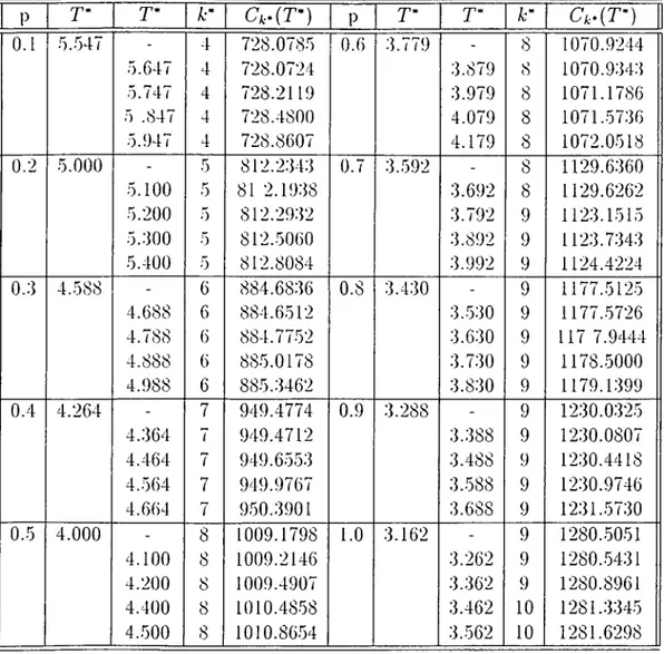
Graphical representation is provide in Figure 3.1.

P T* Ar* Ck>(T·) P T* k· Ci-(T·) 0.1 5.547 - 4 728.0785 0.6 3.779 - 8 1070.9244 5.647 4 728.0724 3.879 8 1070.9343 5.747 4 728.2119 3.979 8 1071.1786 5 .847 4 728.4800 4.079 8 1071.5736 5.947 4 728.8607 4.179 8 1072.0518 0.2 5.000 - 5 812.2343 0.7 3.592 - 8 1129.6360 5.100 0 81 2.1938 3.692 8 1129.6262 5.200 5 812.2932 3.792 9 1123.1515 5.300 5 812.5060 3.892 9 1123.7343 5.400 5 812.8084 3.992 9 1124.4224 0.3 4.5S8 - 6 884.6836 0.8 3.430 - 9 1177.5125 4.688 6 884.6512 3.530 9 1177.5726 4.788 6 884.7752 3.630 9 117 7.9444 4.888 6 885.0178 3.730 9 1178.5000 4.988 6 885.3462 3.830 9 1179.1399 0.4 4.264 - 7 949.4774 0.9 3.288 - 9 1230.0325 4.364 7 949.4712 3.388 9 1230.0807 4.464 7 949.6553 3.488 9 1230.4418 4.564 7 949.9767 3.588 9 1230.9746 4.664 7 950.3901 3.688 9 1231.5730 0.5 4.000 - 8 1009.1798 1.0 3.162 - 9 1280.5051 4.100 8 1009.2146 3.262 9 1280.5431 4.200 8 1009.4907 3.362 9 1280.8961 4.400 8 1010.4858 3.462 10 1281.3345 4.500 8 1010.8654 3.562 10 1281.6298

Table 2.3: Example of Model A Policy II

Results of the e.xample states that, as the probability of critical failure increases, replacement age T decretases. In addition to that, number of critical failures for replacement increases. Since cost of critical failure is increasing due to the occurrence of more critical failures, total cost is also increasing

CHAFTER 2. OPTIMAL REPLACEMENT POLICIES

in p. Notice that the cost figures vvitli optima! A:’ are very close to those at

T “ which corres|)on(ls to the model when k —> 'oo; i.e. wlien the number of

critical failures are not considered in the model. Such an observation leads that number of critical failures as a decision variable is not that much important at least for this specific example.

CHAPTER. 2. OPTIMAL REPLACEMENT POLICIES :C)

2.2.2

M o d el B

In the previous model, the system under consideration is replaced at age Tor at Arth critical failure, whichever occurs first. In model B, it is assumed that the system under consideration is replaced at the first critical failure which occurs after age T. Objective of this model is to find the age Twhich minimizes the average long-run maintenance cost.

Let r Ije the duration of the time from T t(j the occurrence of the first critical failure and h't Fr(f.) be its distribution function, Then;

Frit) = V {t < t ) = [ - = 1 - e - r [ « ( T + r ) - f i ( T ) ] ^

with probability density function:

f,{t) = pr{T + t)e-^mr+t)-R{r)]

• Expected length of the replacement cycle: The system is in operation

T T units of time. Then expected length of the replacement cycle is; £[RC] = T + 8[t] where. f ( r ) =

r

• Expected cost until replacement: Total cost of repairing both critical and non-critical failures together with replacement cost are considered for the expected cost until replacement.

.Since the system is replaced at the time of the first critical fiiilure that occurs after time T, the expected number of critical failures in a replacement cycle is given by [2.17] as ¿’[M;.] = pR{T). Thus expected cost for critical failure repair is;

CHAPTER 2. OPTIMAL REPLACEMENT POLICIES M)

Expected number of non-critical failures is o[yV7'^r]· Noting from (2.1(S) that, = (1 -p)R{T)·, = r i ( J V i « k = iW n (i) J 0 roo = ( l- p ) [ /? ( T ) + (l/p)] (2.48)

Thus, the ex])ectecl cost for non-critical failure repairs until replacement is;

<■„(1 - r t [ « ( 7 ’) + (l/p)l (2.49)

Finally, from (2.47), (2.49) and introducing replacement cost,

'.[total co.s/i] = c,npR{T) + c,j( I - p)[R(T) + ( l/p)] + c r (2.50)

Let C{T) be the average long-run maintenance cost function of a system subject to replacement at the first critical failure occurs after time T. Then from (2.24) and (2.50); cwpRiT) + Coil - p m T ) + (l/p)] + CR C{T) = Note that X e_ -P^O)da ^~^Co -)- Cr C(0) =

and (2.51) is decreasing if,

T

epiMT) j : - e-P^nu)du

and increasing il,

T ePl^C') e-pf^C)du j ; - e-pBOdu - [pR{T) - l ] < p - (p/i(T) - 1] > p (1 - p)cq 4- pcR Pi-m + ( 1 ~ p)Co (1 - p)cq + pCR pc,n + (1 - p)co (2.51)

For the determination of optimal T* which minimizes (2.51, the following theorem is given.

CHAPTER 2. OPTIMAL REPLACEMENT POLICIES ;{7

T h e o re m 2.3 i) The value of T* vjliicli aiinitnizes (2.51) is the value oj T

which satisfies;

[CntP + Cq(1 - p)]

pgp/i(T) = C{T) (2.52)

a) There exists at most one value for T" and it is unique.

in) If no solution to (2.52) exists then there is no need to replace the system.

P ro o f, i) DifFerentiating (2.51) with respect to T and ecpiatiiig to zero gives (2.52). Tims, it is optimal to replace the system at the first critical failure occurs after time T* which siitisfies (2.52).

ii) Let tp(T) be defined as; [r.np + co( 1 - p)]

0 (T) = - C{T) (2.53)

pepf^O f j ‘e

[^toP + <’o( 1 — />)] CmPR{T) + C'o( 1 — p)[R{T) + ( 1/p)] + Cfi p(,pR{T) e~^’^C)du T + eP^H) f'p t-pJ^Odu

For r = 0, t/’(0) = {crn - c n ) ! U ^ < 0 and, dHT) r { T ) [ T + H { T ) Y dT where pMP{T) . c ,[ p - p H { T ) -{ T + H { T ) )] + [c,R{T)+c>]pHiT) > 0 H{T) = f^ e-P^^^'^\lu cl = c,np + Co(l - p) c2 = Co((l — p)/p) + Cfi

Thus il'{T) can cross zero at most once. Also, t/fiT) oo as T —> oo, T ‘ is unique.

iii) If no solution to (2.52) exists, then T* = oo so that it is better to use the system forever or until it bo'comes unusable.

CHAPTER 2. OPTIMAL REPLACEMENT POLICIES

Example

In order to demonstrate the use of model, consider a system with VVeibull lifetime distribution having shape parameter <y = 2 (relevant information was given on page 25).

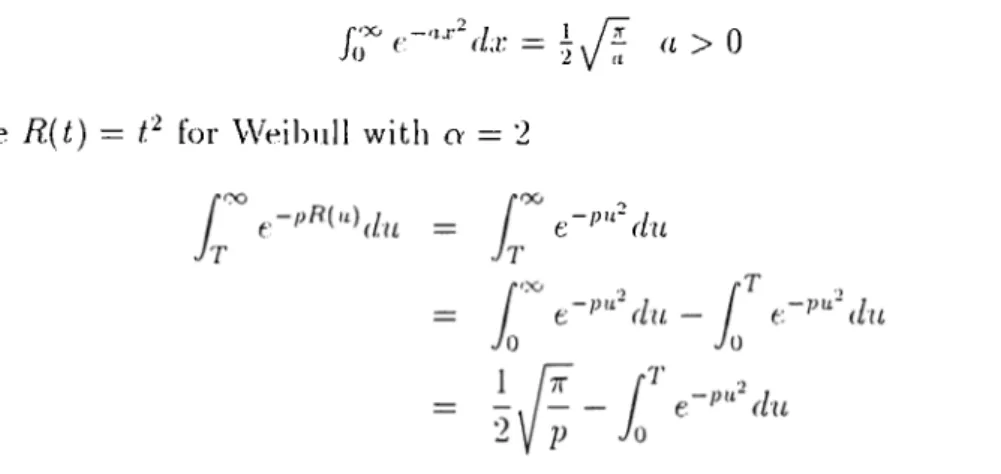
Value of T* can be found by numerical search. For the easiness of compu­ tation, the integral in the denominator of the cost function can be rewritten l)y using integral tallies;

/,;^c ·'·'■■ dx· = a > 0 since R{t) = C for Weibull with cv = 2

(2.54)

Table 2.4 summarizes the values of T* for two different cost combiiuition s.

Co - 50 c,„ = 200 C R = 2000 Co = 10 Cm = 30 C R = 50 P C ( r ) C{T') 0.1 4.500 692.6314 0.720 43.7929 0.2 4.285 763.0043 0.881 44.7901 0.3 3.994 830.2513 0.950 44.0860 0.4 3.723 893.2245 0.980 44.4863 0.5 3.471 952.5145 0.994 45.2979 0.6 3.260 1008.6749 1.000 46.2896 0.7 3.080 1062.1297 1.023 47.3642 0.8 2.920 1113.2049 1.107 48.4769 0.9 2.780 1162.1741 1.198 51.6038 l.O 2.650 1209.2557 1.214 56.7684

CHArTEIl 2. OPTIMAL llEPLACLMENT POUCIES :{!)

As can h(' expected, while the probability of critical failure occurrence in­ crease, the o|)tiinal T ‘ is decreased. The case /) = 1 is not simply the classical age replacement model since under age replacement the system is replaced at a failure or at the age, whichever occurs first. But, here there may occur expectedly R(T) number of failures until replacement. In the above case ex­ pected number of failures in (0,2.650) for p — l,Co = 50,c„i = 200,ch = 2000 is 2.650^ ~ 7. For the other cost figures expected number of failures is ap- ])roximately 1. Graphical representation of the results is providtxl in Figure 3.1.