Frequency allocation and clustering in frequency hopping AD HOC networks

(1)

FREQUENCY ALLOCATION AND CLUSTERING IN FREQUENCY HOPPING AD HOC NETWORKS

RAVS¸AN AZ˙IZ

MASTER’S THESIS

ELECTRICAL AND ELECTRONICS ENGINEERING

TOBB UNIVERSITY OF ECONOMICS AND TECHNOLOGY INSTITUTE OF ENGINEERING AND SCIENCE

JULY 2015 ANKARA

(2)

Approval of the Institute of Engineering and Science.

Prof. Dr Osman ERO ˘GUL Director

I certify that this thesis satisfies all of the requirements of the Master’s degree.

Prof. Dr. Murat ALANYALI Department Chair

I certify that this thesis titled FREQUENCY ALLOCATION AND CLUS-TERING IN FREQUENCY HOPPING AD HOC NETWORKS prepared by RAVS¸AN AZ˙IZ certifies as a Master’s thesis.

Assoc. Prof. Dr. Tolga G˙IR˙IC˙I Supervisor

Examining Committee Members

Chair : Asst. Prof. Dr. ˙Israfil BAHCECI

Member : Assoc. Prof. Dr. Tolga G˙IR˙IC˙I

(3)

TEZ B˙ILD˙IR˙IM˙I

Tez i¸cindeki bütün bilgilerin etik davranı¸s ve akademik kurallar ¸cer¸cevesinde elde edilerek sunuldu˘gunu, ayrıca tez yazım kurallarına uygun olarak hazırlanan bu ¸calı¸smada orijinal olmayan her türlü kayna˘ga eksiksiz atıf yapıldı˘gını bildiririm.

I hereby declare that all the information provided in this thesis has been obtained with rules of ethical and academic conduct and has been written in accordance with thesis format regulations. I also declare that, as required by these rules and conduct, I have fully cited and referenced all material and results that are not original to this work.

(4)

¨

Universitesi : TOBB Ekonomi ve Teknoloji Üniversitesi Enstitüsü : Fen Bilimleri

Anabilim Dalı : Elektrik ve Elektronik M¨uhendisli˘gi Anabilim Dalı Tez Danı¸smanı : Do¸c. Dr. Tolga G˙IR˙IC˙I

Tez Türü ve Tarihi : Yüksek Lisans – Temmuz 2015

Rav¸san AZ˙IZ

FREKANS ATLAMALI TASARSIZ A ˘GLARDA DA ˘GITIK FREKANS TAHS˙IS˙I VE ¨OBEKLEME

¨ OZET

Frekans atlama, haberle¸smede giri¸simi kontrol etmek ve frekansı tekrar kullanmak i¸cin kullanılan bir tekniktir. Askeri a˘glarda frekans atlama ile giri¸sim azaltılabilir ve sinyal bozucuların sistemler üzerindeki kötü etkileri en aza indirilebilir. Do˘gru frekans tahsisi yapabilmek, askeri a˘glarda güvenlik, gürbüzlük ve en kötü durumdaki kullanıcının bile ba¸sarım sa˘glaması bakımından önem kazanmı¸stır. Askeri a˘glar genellikle merkezi olmayan tasarsız a˘glardır. Tasarsız a˘glarda hiyerar¸si ve a˘g kontrolünü sa˘glamada öbekleme kullanılabilir. Öbeklemenin ba¸slıca faydaları, giri¸simi azaltmak, gü¸c ve kanal verimlili˘gi sa˘glamak ve da˘gıtık algoritma uygulamayı mümkün kılmak olarak sıralanabilir.

Bu ¸calı¸smada frekans atlamalı tasarsız a˘glarda; ba˘glantılı öbekleme ve frekans tahsisi problemleri ele alınmaktadır. Frekans tahsisi i¸cin; a˘g bilgisine dayalı merkezi ¸cözüm, karı¸sık tamsayılı programlama ve da˘gıtık olarak uygulanabilir bir algoritma ¨

onerilmi¸stir. Obekleme i¸¨ cin tamsayı programlamaya dayalı bir optimal yöntem ve da˘gıtık olarak uygulanabilir bir algoritma önerilmi¸stir. Bu yöntemler TDMA-tabanlı bir tasarsız a˘g benzetim ortamında test edilmi¸stir. Yapılan benzetimlerle, önerilen da˘gıtık-uygulanabilir algoritmaların merkezi ¸cözümlere olduk¸ca yakın ba¸sarıma sahip oldu˘gu gösterilmi¸stir.

Anahtar Kelimeler: Kablosuz, Frekans Atlama, Frekans Tahsisi, Tasarsız A˘glar, ¨

(5)

University : TOBB University of Economics and Technology

Institute : Institute of Natural and Applied Sciences

Science Programme : Electrical and Electronics Engineering

Supervisor : Assoc. Prof. Tolga G˙IR˙IC˙I

Degree Awarded and Date : M.Sc. – JULY 2015

Rav¸san AZ˙IZ

FREQUENCY ALLOCATION AND CLUSTERING IN FREQUENCY HOPPING AD HOC NETWORKS

ABSTRACT

In this work, clustering and frequency allocation in TDMA-based frequency-hopping ad hoc tactical networks are examined. We propose Mixed Integer Linear Programming based optimal clustering solution along with a distributed load-balanced clustering algorithm. As for the frequency hop set allocation, we first propose a centralized global algorithm and a centralized MIQP solution based on full channel information. Then we propose a distributed channel allocation algorithm. Simulation results reveal that the proposed algorithms perform very closely to the benchmark solutions in terms of throughput, delay and hop count performance.

Keywords: Wireless, Frequency Hopping, Frequency Allocation, Ad Hoc Network, Clustering.

(6)

ACKNOWLEDGEMENT

I would like to express my gratitude to my supervisor Assoc. Dr. Tolga G˙IR˙IC˙I for the useful comments, remarks and engagement through the learning process of this master thesis. Furthermore I would like to thank Tolga Numano˘glu, G¨uven Yenihat and Halime Koca for their contribution and participation in the project No.1538.STZ-2012.2 under the scope of the SANTEZ programme. I am grateful to TOBB ETU, it’s staff and it’s administration for providing me the opportunity to perform and conduct the research for this thesis. I would like to thank my loved ones, who have supported me throughout entire process, both by keeping me harmonious and helping me putting pieces together. I will be grateful forever for your love.

(7)

LIST OF FIGURES

1.1 Military Communication Network . . . 2

1.2 Clustering Structure . . . 4

1.3 Frequency Hopping . . . 6

1.4 System Topology. . . 9

1.5 Connected Distributed Clustering Topology. . . 10

2.1 Cluster Structure Obtained From Optimization Problem . . . 15

2.2 Cluster Structure Obtained From Optimization Problem . . . 16

2.3 Distributed Clustering Algorithm Structure . . . 19

2.4 DCA OCA Total Throughput Performance . . . 22

2.5 Throughout Per Cluster for OSC and DCA . . . 23

2.6 Average Hopcount for OSC and DCA . . . 24

3.1 Rugged Terrain . . . 26

3.2 Rugged Terrain(contour line) . . . 27

3.3 Cycle Topology . . . 28

3.4 Clustering Topology for Frequency Allocation in Table 3.2 . . . . 33

3.5 Frequency Algorithm Test . . . 37

(11)

4.2 Network Traffic Example . . . 41 4.3 Clustering Sample . . . 43

(12)

LIST OF TABLES

2.1 Simulation Parameters: Clustering Algorithm Comparison . . . . 20

2.2 Simulation Result: Total Network Throughput of OSC and DCA . 21 2.3 Simulation Result: Total Cluster Count of OSC and DCA . . . . 23

3.1 Frequency Allocation by Centralized Frequency Allocation Algorithm 30 3.2 Frequency Allocation by MIQP-Based Solution . . . 32

3.3 Simulation Parametersi for Frequency Allocation Algorithms . . . 36

4.1 Cluster Members in a Sample Clustering Structure . . . 43

4.2 Routing Information for the Sample Example . . . 44

4.3 TDMA Reservation . . . 45

4.4 Voice Traffic Model . . . 46

4.5 Command & Control Traffic Model . . . 46

4.6 Video Traffic Model . . . 47

5.1 Traffic Parameters for QUALNET Simulation . . . 48

5.2 Results for QUALNET Traffic Simulation . . . 50

5.3 Traffic Simulation Parameters for Different Clusterhead Routing Types . . . 53

5.4 Type 1 Routing Traffic Simulation Results . . . 54

(13)

5.6 Type 3 Routing Traffic Simulation Results . . . 56 5.7 Traffic Simulation Parameters for Clustering Algorithm Comparison 57 5.8 MILP Based Solution Traffic Simulation Results . . . 58 5.9 Distributed Clustering Solution Traffic Simulation Results . . . . 59 5.10 Traffic Simulation Parameters for Different Frequency Algorithms 60 5.11 Traffic Simulation Parameters for Different Frequency Algorithms 61 5.12 Traffic Simulation Results for Different Frequency Algorithms of

the Configuration 2 Video, 4 Command & Control, 10 Voice Source Nodes . . . 62 5.13 Traffic Simulation Results for Different Frequency Algorithms of

the Configuration 2 Video, 5 Command & Control, 10 Voice Source Nodes . . . 67

(14)

5.18 Traffic Simulation Results for Different Frequency Algorithms of the Configuration 2 Video, 6 Command & Control, 10 Voice Source Nodes . . . 68 5.19 Traffic Simulation Parameters for Different Frequency Sets . . . . 69 5.20 Success Rate for Traffic Simulation Over Different Frequency Sets 69

(15)

List of Symbols

Variable Description Related Section xji Connection parameter of node i to cluster j 2

cji Throughput capacity between node i and j 2

Ij Clusterhead parameter of node j 2

Imax Maximum clusterhead count 2

N User set 2

Nmax The maximum users in a single cluster 2

Ci The total throughput of i to its neighbors k 2

Ui The amount of users i exceeds in throughput 2

i∗ _{Potential clusterheads with a value of U}

i 2

N∗ _{Proposed clusterhead set} ₂

CH Clusterhead set 2

fmin Minimum frequency band 3

fmax Maximum frequency band 3

W Bandwidth 3

Nf Frequency band count 3

N0W Additive White Gaussian Noise power 3

P Users power 3

dij Distance between i and j 3

Π Frequency pattern Set 3 Πc Most suitable pattern set for cluster c 3

pic Pattern set allocated to cluster c 3

π Pattern set allocated to all clusters 3 In,k The noise+intereference level n user is exposed at

channel band k

3

hn,m,k The pathloss between user n and m at cgabbel k 3

β1 First sideband coefficient 3

β2 Second sideband coefficient 3

Nc

f,min The minimum frequency band number allocated to a

cluster c

3 Nc

f,max The maximum frequency band number allocated to a

cluster c

3 In The average interference of user n in all channels 3

F (π) The maximum interference of the average user interfer-ence

3 aij The neighbor parameter of cluster i and cluster j 3

(16)

1. INTRODUCTION

1.1 Radio Communication Systems

The scientists who saw and investigated the impacts of electricity and magnetism contributed in the early establishment of radio technology. Maxwell proved the existence of electro-magnetic waves, Faraday proposed that electromagnetic forces extend into the empty space around the conductor, and Hertz produced a set of experiments that validated Maxwell’s theory of electromagnetic radiation where he proved that electromagnetic radiation can travel through free space. Then, Marconi- known as the inventor of radio, pursued the studies and built a wireless telegraphy system using Hertzian waves. Following these successful experiments, the Italian Engineer was able to convince the English authorities of the importance of wireless communication, and this opened an opportunity for long distance communications. Soon, short wave transatlantic success has turned the media industry in broadcasting news and entertainment. This industry has evolved greatly and is continuing to evolve in an increasing pace ever since, with new areas of research available for the motivated scientists and engineers.

1.2 Military Radio Communication Systems

Today, military radio communications systems are used by armed forces to deliver audible and visual information, such that it assures a secure, distributed and a fail-safe end-to-end performance. Its QoS specifications are different than from the industrial use. Military communication equipment are designed to encrypt and decrypt transmissions, and often use different frequencies to send to other radios and to satellites. It is interesting to note that the ideas used for tactical and strategic communication mainly innovate from individuals and private companies.

(17)

As in Marconi’s case, where the Italian navy has shown disinterest to radio communication, often senior officials reject the breakthrough ideas for improving communications.

For security reasons, during a conflict, the military has the tendency to hide information to themselves and seek information about the other at the same time. However communicating information always has a vulnerability which is why military forces stress on secrecy and intelligence.

The increased means in signaling and processing has allowed a continuous improvement in military radio communications, which led the carrying messages to become more complex every day.

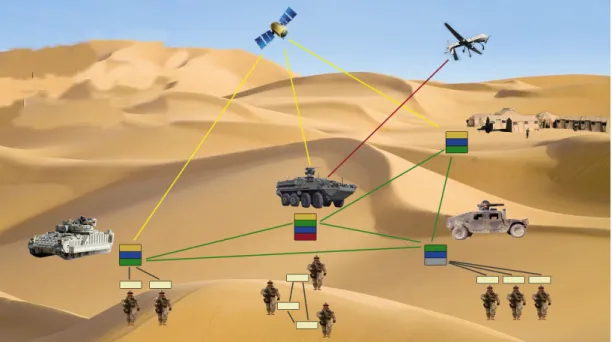
Unlike commercial communication, military radio communication setup usually requires a robust, ad hoc, and a distributed network. These networks should operate under harsh weather and terrain conditions. An example of such a mobile network is shown in Figure 1.1 that can send voice, data and video traffic. The mobile vehicles make the backbone of the network. The members of the network consisting of land, aircraft and marines transfer signals with different radio signal powers.

(18)

The radio communication system discussed in this thesis is considered to be ad hoc. Ad hoc networks are decentralized type of wireless network. They do not rely on a preexisting infrastructure, such as routers in wired networks or access points in managed (infrastructure) wireless networks. This means there are no base stations such as those used in cellular phones. This increases security and robustness. Otherwise, if the network relies on a fixed infrastructure, the breakdown of a single-point of failure of a fixed station can cause the network to go down.

Communication occurs by transferring signals when the users can sufficiently ensure the necessary signal-to-noise ratio threshold conditions. Jammers are used by hostile users to prevent communication by intentional emission of radio frequency to interfere signals with false noise or information. To prevent the side effects of jamming, frequency hopping is used. Frequency hopping is a method of transmitting radio signals by rapidly switching a carrier among many frequency channels, using a pseudorandom sequence known to both transmitter and the receiver. Frequency hopping will be further discussed.

1.3 Clustering

In today’s world, billions of machines are connected to each other, and the increasing trend shows that this number will increase by a factor of five in less than two decades. In this case, a certain grouping schematic has to be applied. Clustering is the task of grouping a set of objects in such a way that objects in the same group named as cluster where clusters are more similar to each other than to those in other groups. In military radio communication, standalone radios are becoming insufficient in providing the required QoS. During a conflict, using centralized planning by using a main base station is inadequate in terms of using the radio spectrum and optimizing the user organization in terms of performance costs. Making a centralized network has the potential of having a single-point-of-failure, where in the case of an attack to the main base station, the majority of the infrastructure might collapse. Hence using clustering in a military radio communication has these several advantages:

(19)

1. It can be applied in a distributed manner . 2. It is power efficient.

3. It is channel efficient. 4. It can decrease interference. 5. It is scalable

Figure 1.2: Clustering Structure

Clusters are distributed in a topology based on their location, their signal strength, closeness to other users and connectivity with respect to the general topology. Cluster architecture facilitates spatial reuse, where members of different distant clusters in the same network can be assigned with the same frequency set, and this increases the system capacity in terms of resource use. Members of the same clusters are close to each other, and they spend less energy transmitting data to each other which extends their lifetime and increases power efficiency. The information is routed over cluster heads. Cluster heads are the main member of the cluster that is responsible for synchronizing, assigning and routing

(20)

transmissions in time division frames. This allows scaling even for large number of users.

A cluster formation can be seen in Figure 1.2. In this example, there are five clusterheads, and every cluster has a clusterheadmember labeled as red. The users connected to the preferred cluster given certain specifications and parameters.

1.4 Frequency Allocation

Frequency allocation is the management and regulation of spectrum of the radio frequency bands of the electromagnetic spectrum. Giving technical and economic reasons, governments allow a certain portion of the radio spectrum for users, companies, and the military to use. The scarcity of the spectrum promotes the bands to be used effectively and this advocates research on using the frequency band efficiently. Military communication frequency allocation generally takes place in the range of 30-512MHz area. Understanding the operational process in planning, managing, and employing this resource is critical to the conduct of providing the QoS and enabling a high performance.

1.4.1 Frequency Hopping

Frequency Hopping Spread Spectrum (FHSS) is a method of transmitting radio signals by rapidly switching a carrier among many frequency channels, using a pseudorandom sequence known to both transmitter and receiver. There exists slow and fast methods of frequency hopping. In slow frequency hopping, a few symbols are sent in a hopping period. In fast frequency hopping a symbol is sent in more than one hopping time. This creates frequency diversity and decreases the interference between the symbols. Though frequency hopping provides an advantage in various cases, it creates an issue of frequency allocation problem. Frequency hopping is widely used in GSM and military applications. Frequency hopping is especially important in GSM systems. The pathloss in radio signals is generally attributed to the Rayleigh Fading Model. In a case where path loss

(21)

is high for a mobile node, information loss can be significant. Frequency hopping can provide frequency diversity and decrease the loss of transmission. The second advantage of frequency hopping is in the ways it can decrease interference. Without frequency hopping, the interference of other signals using the same or similar frequency can have a major impact to communication. The usage of frequency hopping can decrease interference [1]. Moreover, frequency hopping increases the resistance against cross-symbol interference. Fig. 1.3 shows how different frequencies are used in frequency-space time. The carrier frequencies change every hop such that the two close users do not interfere each other.

Figure 1.3: Frequency Hopping

1.5 Literature Analysis

Military tactical ad hoc networks require secure, connected, interference free, fast communication that can be deployed immediately in a distributed manner. The military tactical ad hoc network terminals communicate freely with each other via wireless links by broadcasting radio transmissions within their transmission power range. Usually this requires a multi-hop configuration where packets are routed by forwarding from source over intermediate terminals to the destination [2] [3]. Without the existence of base stations and fixed network infrastructures, careful management of the network is necessary in order to ensure entire area coverage.

(22)

Efficient communication can be supported by developing a wireless backbone architecture [4] [5] [6] [7]. Virtual backbone can be formed by building a Connected Dominating Set (CDS) . With the help of the CDS, routing is easier and can be localized to adapt quickly to network topology changes [8] [9] [10]. Routing messages are only exchanged between the backbone nodes that act as a clusterhead instead of being broadcasted to all the nodes. A clusterhead often serves as a local coordinator for its cluster, performing intra-cluster transmission arrangement, data forwarding, and other duties. Other ordinary nodes behave as a clustermember, which is a non-clusterhead node without any inter-cluster links. It has been shown that cluster architecture guarantees basic QoS performance achievement in a MANET with a large number of mobile terminals [11]. A cluster structure, as an effective topology control means , facilitates the spatial reuse of resources to increase the system capacity. With the non-overlapping multicluster structure, two clusters may deploy the same frequency if they are not neighbouring clusters. A cluster can coordinate its transmission events effectively and decrease transmission collision, making the ad hoc network appear smaller and more stable for each mobile terminal where local changes do not need to be updated by the entire network, and information stored and processed is decreased vastly by each node [12] [13]. The clusterhead can adjust channel scheduling, perform power measurement, maintain synchronization of time division frames, and improve the spatial reuse of the time slots. This makes the clustered network scalable to large numbers of nodes [14].

In the absence of a centralized control, channel assignment in military radio sensor networks is implemented in a distributed manner. Research is being conducted on the problem of interference management in network deployments where terminals communicate using the same frequency bands and can interfere with each other. Interference of transmission signals effect the QoS of the adhoc network system, and in a tactical network packet delivery time thresholds hold vital importance. [15] [16]. Dynamic channel allocation algorithms based on the level of interference measured on each channels has been proposed to static channel allocation and random frequency hooping to reduce the co-channel interference and improve the network performance [17] [18] [19] [20]. Frequency assignment utilization based on signal-to-interference costs have been performed in the frequency assignment

(23)

problem [21] [22] [23]. However, given frequency allocation schemes have not accommodated the requirements of an increasing number of higher data rate devices in a clustering environment. A new way of exploiting available spectrum in a frequency hopping clustered network has been researched in this paper to use the frequency bands opportunistically in a frequency hopping clustered network. One of the favored frequency allocation methods in frequency hopping is simulated annealing. Similarly, this thesis will use a similar technique by creating a benchmark for one of the optimal solutions. Simulated annealing is a probabilistic meta-heuristic method for a global optimization problem by locating a global optimum given a certain function in the large search space. This method helps the testing frequency allocation of a TDMA (Time Division Multiple Access) based applications [24] by creating several frequency patterns and assigning these patterns to users. Simulated annealing has been used in GSM networks to allocate frequencies in a frequency hopping environment [22].

So far, most of the work for frequency hopping has been made for cellular networks. In cellular networks, the increase in demand leads to an insufficient frequency band and the reuse of frequency spectrum becomes important. When the frequency reuse is not optimized, the interference levels can increase high such that it decreases the performance. In frequency hopping networks, the frequency reuse can be set to minimize the interference levels, using simulated annealing [25] or by obtaining an optimal solution by MLIP.

1.6 System Model

We have selected a distributed TDMA cluster approach to supply requirements of efficient network resource control and multimedia traffic support. Deployed terminals comprises a number of N units that are distributed randomly, each equipped with a 10W and 50W cognitive radio devices. They can send voice, data and video packets to their destinations as shown in Figure 1.4. The spheres represent the users transmission range, whereas the green arrows indicate the type of packets being sent and the origin-destination pair.

(24)

Figure 1.4: System Topology.

In the simulations, we consider around 200 nodes distributed in a rectangular area of 12 × 16 km2_{. We assume that each node knows its neighbors based on}

a neighbor discovery process. We consider a frequency hopping network , where each device can tune only on a single channel in a single slot period, and can both transmit and receive in that channel. Channel loss is calculated with respect to the distance and frequency, by using Rayleigh Fading Model and location advantage [−10dB, +10dB] in accordance to the node position. Via clustering, the whole population of nodes is grouped into clusters,as shown in Figure 1.5 . Each clusterhead, labeled red, acts as a regional broadcast node, and as a local coordinator to enhance channel throughput. Time-division scheduling is enforced within a cluster, where clustermembers transmit their packages via clusterheads using the allocated set of frequencies at their reserved time slots. The network does not permit two clustermembers of the same cluster to transmit packets over to the clusterhead at the same time slot, however multiple transmissions can be accomplished in a single time frame. Resource management is made by dynamic slot and frequency reservations. Spatial reuse of time and frequency slots is facilitated across the clusters. This allows distant clustermembers to use the same frequency bands at the same time. The main idea is to provide a feasible interconnected clustering algorithm that is stable, excludes single points

(25)

Figure 1.5: Connected Distributed Clustering Topology.

of failure on heavily loaded traffic and is easy on topological changes. At this stage node mobility is not considered that makes clustering more challenging since the node membership will dynamically change, forcing clusters to evolve over time. However, our proposed clustering algorithm can be modified to support mobility and cluster maintenance. The model supports various applications in a tactical military ad hoc network, including voice, command and control, ftp and video. We represent the ad hoc wireless network by a directed graph G(V ). Each node v ∈ V = 1, ..., n symbolizes a terminal with (possibly varying) circular transmission range Rt(v) and a carrier sensing range Rh(v). The graph

connectivity is given by a connectivity matrix A. The adjacency matrix A ∈ G(V, E) is a matrix with rows and columns labeled by the graph vertices V, where the matrix entry av,u is 1 or 0 if nodes v and u are unidirectionally connected or

not. An edge (v, u) is bidirectional if both au,v and av,u = 1 are 1.

Each node v transmits with a rate rv,u to its neighbor u ∈ Ne(v). The available

transmission bit rate rv,u is determined through the link condition depending on

the transmission power, distance between the node v and u and the resulting loss rate on that link resulting from interference. Our model includes the effects of interference therefore the transmission bit rates are not fixed.

(26)

1.7 Motivation

Today’s modern military has access to real-time data with technologies such as data networking, GPS, real-time video feeds from UAVs, and satellite intelligence. However, supplying this information to the users of the fighters at the edge of the network is still an issue. Making real-time voice, data and streaming video to a user at the edges of a network is a challenging task. Providing a firm networking infrastructure in place on the battlefield is crucial. By producing protocols that can be implemented to clustered groups to decrease interference, increase routing performance and connectivity will help mobile soldiers to obtain high-performance to deliver the information they need. Hence this thesis is motivated to find solutions for military radio communication such that

• The proposed clustering and frequency allocation algorithms are dis-tributed.

• Frequency reuse efficiency is maximized.

• Sufficient transmission takes place in the worst case scenario. • Traffic is routed in the given delay parameters.

1.8 Thesis Contents and Contributions

This research is supported jointly by the Turkish Ministry of Science, Industry and Technology and Aselsan Inc., through SANTEZ program, project No. 1538.STZ-2012.2.

A conference paper for MILCOM 2015 on frequency allocation and clustering for tactical radio networks has been written and has been accepted.

In this thesis, I will first propose a connected clustering scheme by forming a virtual backbone of a CDS with different transmission ranges in order to maximize throughput cost of the network. The first scheme is called optimal

(27)

static clustering. The optimal cluster placement that maximizes the total throughput by formulating a centralized clustering problem as a mixed linear integer programming (MLIP)is determined. Then, in the second scheme, named distributed clustering algorithm, a distributed clustering algorithm that satisfies the connectivity constraint using a marking process where the cluster formation is amenable to distributed implementation is proposed. When the network is deployed randomly such that clusterheads are concentrated in a particular part of the network forming an unbalanced cluster formation some portion of the network may become unreachable or if the resulting distribution of the clusterheads in multi-hop communication, the nodes closer to the clusterhead are under a heavy load as all the traffic is routed from different areas of the network to the clusterhead through the clustermembers [26]. For this reason, a local and dynamic clustering algorithm that is applicable for TDMA-based load balanced wireless ad hoc networks and that is adaptable to topology changes will be proposed. Furthermore, the clusters may overlap, which creates undesirable interference effects. To minimize the effects of interference, we first propose a global centralized frequency hop set allocation scheme, and then formulate a distributed algorithm that allocates available frequencies to minimize the potential interference caused in the network. To the best of our knowledge, no clustering approach in terms of connectivity constraint and interference effect among neighbouring links for frequency hopping tactical ad hoc networks have been previously proposed in the literature in the context of optimal integer programming. These schemes are tested in TDMA-based computer simulation environment. Numerical results reveal that the distributively implementable algorithms are close to the centralized ones, in terms of transmission rate performance.

This thesis is organized as follows. Section 2 describes the optimal and local algorithmic model of the distributed connected clustering problem. Section 3 presents the optimal and local algorithms for the distributed frequency hop set assignment problem. Section 4 describes the routing considerations and describes the network traffic. Numerical results are given in Section 5, with a conclusion drawn in Section 6.

(28)

2. CLUSTERING

Clustering objective is set in order to facilitate meeting the application require-ments, where sensitivity to data latency, intra and inter-cluster connectivity and the length of the data routing paths are considered as criteria for CH selection and node grouping. A cluster structure, as an effective topology control means , facilitates the spatial reuse of resources to increase the system capacity. A cluster can coordinate its transmission events effectively and decrease transmission collision, making the ad hoc network appear smaller and more stable for each mobile terminal where local changes do not need to be updated by the entire network, and information stored and processed is decreased vastly by each node. This vastly decreases the overheads used and allows more information to be sent in the data packets. To this end, an optimal MLIP-based clustering that maximizes network throughput will be considered. Then our proposed algorithm that provides strong connectivity with a load balanced property will be explained. The MLIP clustering and the algorithms are described below:

2.1 Optimal Static Clustering

The optimal static clustering that maximizes the network throughput between the clusterhead and its members will be the benchmark for our proposed distributed clustering algorithm. The objective function is defined in (2.1) , where xji

represents the connectivity of node i to node j (clusterhead), where 1 denotes connected or 0 not connected. cji is the total throughput of node i to node

j. Binary vector Ij indicated whether node j is selected as clusterhead or not.

Constraints are put to obtain a global unique solution; (2.2) enforces each node to connect to a single clusterhead, (2.3) tells that cluster members can connect only to clusterheads, (2.4) sets the maximum number of clusterheads, (2.5) sets the maximum number of cluster members in a single cluster.

(29)

max x,I ( X i∈V X j∈V xjicji) (2.1) X j∈V xji = 1, ∀i ∈ V (2.2) Ij ≥ xji, ∀i, j ∈ V (2.3) Imax ≥ X j∈V Ij (2.4) Nmax ≥ X i∈V xji, ∀j ∈ V (2.5)

In our previous examinations, clusters were not assigned to have full connectivity. It is important that there should be at least one route from any edge node to another. For this we need to have a connected graph. This can be obtained by ensuring a connected dominating set. To form a connected dominating set, we need several more constraints. The adjacency matrix A = (aij), of G is a N × N

binary matrix, where aij = 1 if there is an bidirectional edge linking nodes i and

j in E and 0 otherwise. We guarantee that all clustermembers have an adjacent clusterhead in Equation (2.6). The capacity for i = j of cij is equal in Equation

(2.6) and does not impact on the throughput maximization. We also define a f lowmatrix, F = (fij), where fij represents the flow from node i to node j. A

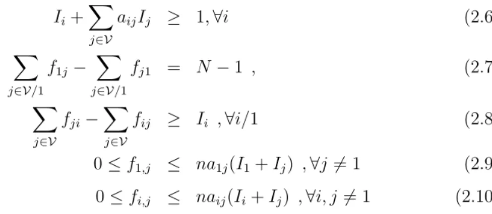
connected subgraph should be able to send flow from a source node to any other nodes using clusterhead as intermediate nodes. Constraint (2.7) makes sure that the source node produces sufficient flow to supply at least one unit of flow to all other clusterheads. Constraint (2.8) ensures each clusterhead uses at least one unit of flow. Flow is positive and can travel along a valid edge shown in (2.9) and (2.10). Note that we initiate flow from node 1. Node 1 is the initiator node in the distributed environment.

(30)

Ii+ X j∈V aijIj ≥ 1, ∀i (2.6) X j∈V/1 f1j − X j∈V/1 fj1 = N − 1 , (2.7) X j∈V fji− X j∈V fij ≥ Ii , ∀i/1 (2.8) 0 ≤ f1,j ≤ na1j(I1+ Ij) , ∀j 6= 1 (2.9) 0 ≤ fi,j ≤ naij(Ii+ Ij) , ∀i, j 6= 1 (2.10)

The identified problem for the given constraints has been solved by using the tools of GAMS and MATLAB.

Figure 2.1: Cluster Structure Obtained From Optimization Problem The best clustering optimization problem actually varies based on factors affecting on data rates, interference, routing and hop counts. In this solution we maximize only the data rates. In the local sense it might not be practical. For instance, if

(31)

two close users that are communicating with each other get assigned to different clusters, their end-to-end delay will increase. A topology that might give a lesser total throughput can be more efficient in special cases in terms of traffic delay. Nevertheless, this benchmark serves well. It will assign close users together, and this will prevent high interference levels. A solution example is shown in Figure 2.1. Each graph indicates a cluster, and shows the assigned members in the topological area. Clearly, the radios close to each other are assigned together. A CDS provides a guaranteed connection of clusterhead members for a given SNR threshold. This ensures a distributed hierarchical setup decreasing the interference levels. Indeed a CDS is ensured, however, there can be still a single-point-of-failure. The topology and this algorithm usually picks clusterheads such that the connectivity is either a mesh network, or there is at least two paths for clusterheads as seen in Figure 2.2. This notion will be further investigated as a future work.

Figure 2.2: Cluster Structure Obtained From Optimization Problem

2.2 Distributed Clustering Algorithm

The distributed clustering algorithm has been formulated to work for ad hoc distributed networks. Similar to optimal static clustering, the distributed

(32)

clustering algorithm attempts to formulate a infrastructure that ensures a CDS. A common virtual backbone building algorithm consists of constructing a Minimal Independent Set (MIS) by initiating a spanning tree then connecting the left over nodes to complete connectivity [27]. All nodes in MIS set are colored black and other nodes are colored gray. In the second phase, all black nodes are connected by finding a gray node w that is a clustermember of v in and a neighbor of the clusterhead u and color this node blue. Our approach in our algorithm aims to completely connect all nodes by growing a dominating set that locally maximizes throughput and checks the cluster density with respect to other elected clusterheads (backbone nodes). The load balancing throughput maximization in connected clustering algorithm has not been studied in other literature CDS algorithms.

The Distributed Clustering Algorithm (DCA) has two phases. Initially all nodes are colored white. The first phase is to initiate the clustering from an initiator node (without loss of generality, node 1) , which is typically a 50W node. The initiator node is marked black, and its neighbors (such that a1i = ai1) are marked

gray (Lines 2-6). In the second phase, we will change some grey nodes to black according to a certain rule. A gray node becomes a potential CH if it has at least one white neighbor (Lines 8-12). The potential clusterheads in the set CHpot

broadcast their status and these gray nodes are elected as the clusterhead if it is the only node broadcasting itself as a potential CH or if it has the highest total rate Ci to their white neighbors, among other potential CHs (Lines

13-15). In a protocol, this can be coordinated by the initiator node. If a gray node is elected as a CH it performs two tasks. Firstly, it connects the white neighbors and marks them gray (Lines 16-20). Secondly, it checks the density of neighbor clusters and transfers nodes from denser populated clusters if it is able to provide better rates/SNR (Lines 21-28). In a protocol this can be achieved by a clustermember measuring received SNR and sending a connection request to the CH having fewer nodes and providing the best SNR. This will balance CH loads and improve the overall throughput. Note that interference, i.e. the signtal to noise interference (SINR) levels are not included in the process of swapping nodes between newly elected clusterheads. The process of election of CHs from the gray nodes continues until all white nodes are colored black or grey.

(33)

Algorithm 1 : Distributed Clustering Algorithm (DCA) 1: Initialize W = N , G, B, CHpot = ∅, chi = 0∀i ∈ N

First Phase: 2: for ∀i s.t. a1i= ai1= 1 do 3: G = G ∪ i 4: chi = 1 5: Nuser 1 = N1user+ 1 6: end for Second Phase:

7: while ∃i ∈ G, j ∈ Ws.t.aij = aji = 1 do

8: for ∀i ∈ G do 9: if ∃j s.t. aij = aji = 1 and j ∈ W then 10: CHpot = CHpot∪ i 11: end if 12: end for 13: Calculate Ci = P j∈Wcijaijaji, ∀i ∈ CHpot

14: i∗ = arg maxi∈CHpot{Ci}

15: B = B ∪ i∗ 16: for ∀j ∈ W and aji∗× a_i∗_j = 1 do 17: G = G ∪ j 18: chj = i∗ 19: Nuser i∗ = N_iuser∗ + 1 20: end for 21: for ∀k ∈ G do 22: if SN Ri∗_,k > SN R_ch k,k then 23: if N_iuser∗ < N_chuser k then 24: N_iuser∗ = N_iuser∗ + 1 25: Nuser chk = N user chk − 1 26: chk = i∗ 27: end if 28: end if 29: end for 30: end while

(34)

Figure 2.3: Distributed Clustering Algorithm Structure

An example of the clustering structure created by a distributed clustering algorithm is shown in Figure 2.3. Just like the optimal clustering algorithm, the clustering is formed by neighbors close to each other. This shows a positive effect in terms of throughput maximization.

2.3 Comparison of Static Clustering Algorithm

to Distributed Clustering Algorithm

This section will compare the static optimal clustering algorithm as a benchmark to the proposed distributed clustering algorithm in terms of performance metrics of hop count and throughput maximization.

The global static maximization parameter aimed to maximize the total troughput of the network. The first performance parametric for distributed algorithm is to compare the equation (2.11)

(35)

(X

i∈N

X

j∈N

xjicji) (2.11)

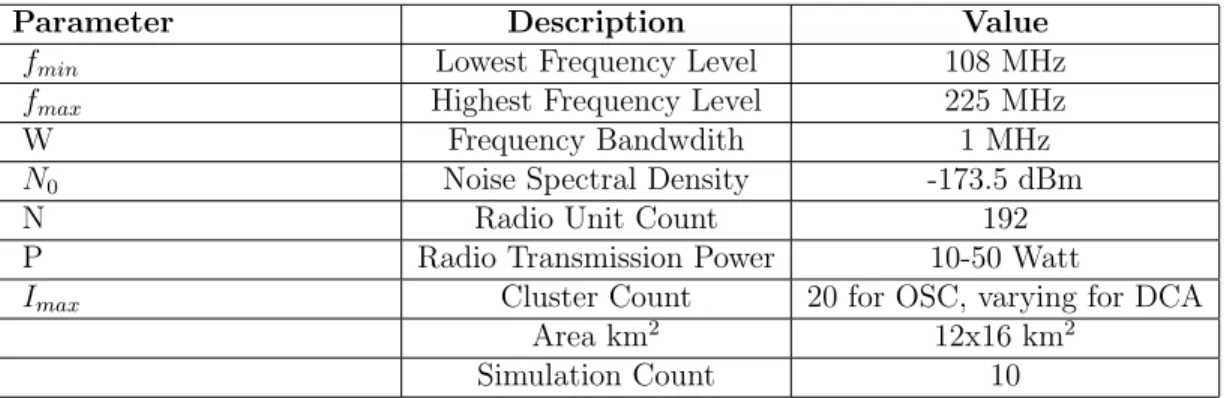
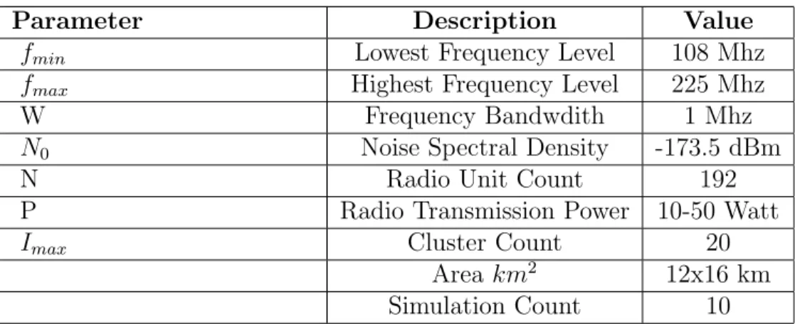
Table 2.1: Simulation Parameters: Clustering Algorithm Comparison

Parameter Description Value fmin Lowest Frequency Level 108 MHz

fmax Highest Frequency Level 225 MHz

W Frequency Bandwdith 1 MHz N0 Noise Spectral Density -173.5 dBm

N Radio Unit Count 192

P Radio Transmission Power 10-50 Watt

Imax Cluster Count 20 for OSC, varying for DCA

Area km2 _{12x16 km}2

Simulation Count 10

2.3.1 Simulation Parameters

Parameters within the two algorithms are equal. However, in distributed algorithm, the cluster count varies depending on the topology. To give a more reliable result, the throughput will be normalized by dividing the total throughput value by the amount of originated cluster count. The simulation parameters are given in Table’ 2.1. In distributed algorithm, we want to stress on connectivity, and there are certain cases when there are edge users left over at the end of the clustering iteration. Our algorithm attempts to load balance this situation by providing loaded cluster members to newly formed clusters. However, at extreme cases it is inevitable that there exists isolated clusters with one or two members.

2.3.2 Results

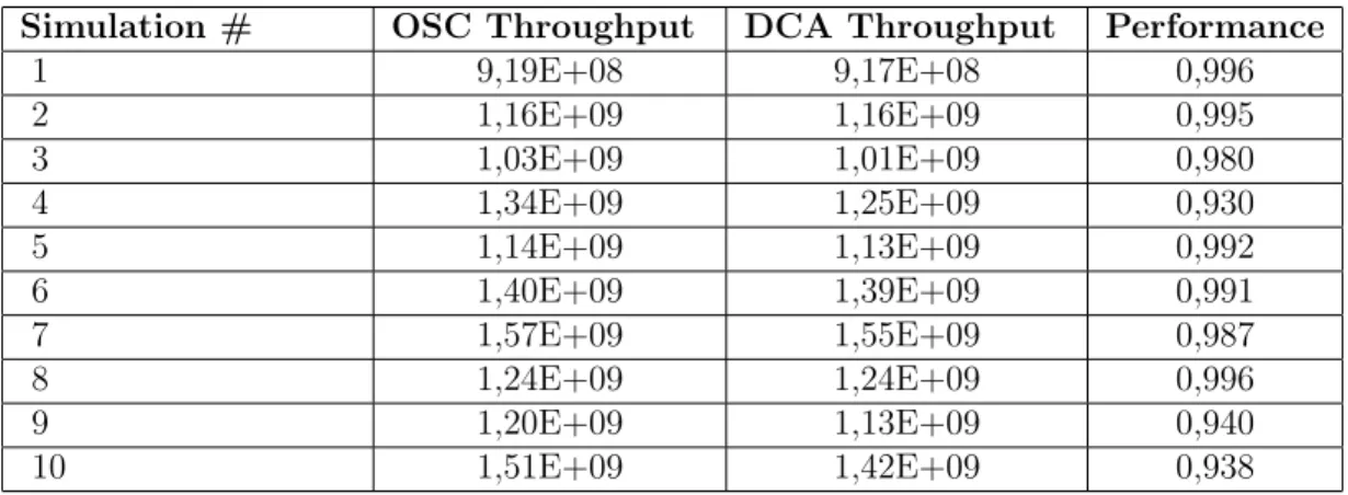
The algorithms were run for 10 different topologies. The total network throughput comparison is given in Table 2.2.

It can be concluded that the suggested DCA clustering algorithm is sufficiently strong in obtaining a high throughput with respect to our proposed benchmark.

(36)

Table 2.2: Simulation Result: Total Network Throughput of OSC and DCA

Simulation # OSC Throughput DCA Throughput Performance

1 9,19E+08 9,17E+08 0,996 2 1,16E+09 1,16E+09 0,995 3 1,03E+09 1,01E+09 0,980 4 1,34E+09 1,25E+09 0,930 5 1,14E+09 1,13E+09 0,992 6 1,40E+09 1,39E+09 0,991 7 1,57E+09 1,55E+09 0,987 8 1,24E+09 1,24E+09 0,996 9 1,20E+09 1,13E+09 0,940 10 1,51E+09 1,42E+09 0,938

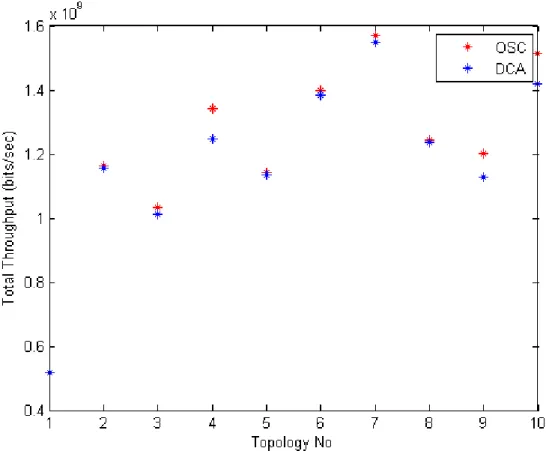
90% of the simulations were above the 0.95 performance rate. This is graphically represented in Figure 2.4.

It should be noted that OCA has a fixed 20 clusters per algorithm while DCA had a varying cluster count shown in Table 2.3. This constraint was normalized by obtaining the total throughput per cluster. Edge clusters decrease the rate for some of the DCA performance in comparison to OSC shown in Figure 2.5. Next, the second important metric in terms of network performance is the hop-count. Hop is one portion of the path between source and destination. Data packets pass through their clusterheads, and other clusterheads as gateways on the way. Each time packets are passed to the next device, a hop occurs. The hop count refers to the number of intermediate users through which data must pass between source and destination, rather than flowing directly over a single broadcast. In a wireless network, the hop-count by itself is not used for determining the optimum network path, as it does not take into consideration the speed, load, reliability, or latency of any particular hop, but merely the total count. Nevertheless, in terms of clustering and comparison of DCA and OSC, it is an important performance metric to show how much loaded the system can get. Since we are using a TDMA approach, the hop-count will be of use.

We first observe the total throughput performance of the proposed and benchmark clustering schemes. Total throughput is measured as the sum of throughput from each node to its respective CH. The total throughput in Fig 2.4 shows that the

(37)

Figure 2.4: DCA OCA Total Throughput Performance

proposed clustering algorithm is in the 5% range of the MILP-based solution. The hop-performance of the distributed clustering have been carried out by testing the average hop count of the entire network for every pair of nodes. Fig 2.6 shows that our Distributed Clustering Algorithm hop-count performance is in the 5% range of the proposed benchmark algorithm.

(38)

Figure 2.5: Throughout Per Cluster for OSC and DCA

Table 2.3: Simulation Result: Total Cluster Count of OSC and DCA Simulation # OSC Cluster Count DCA Cluster Count

1 20 22 2 20 19 3 20 20 4 20 20 5 20 19 6 20 22 7 20 21 8 20 21 9 20 18 10 20 18

(39)

(40)

3. FREQUENCY ALLOCATION

The concepts of frequency allocation and frequency hopping were discussed previously. In this section, the algorithms used for benchmark will take place. Again, similar to the clustering chapter, one of the benchmark solution is solved by a MIQP approach on GAMS. The formulation of the two benchmark algorithms and one distributed algorithm will be shown and then the algorithms will be compared on a basic interference to noise ratio test.

3.1 System Model

N users are randomly distributed one the surface shown in Figure 3.1 ve Figure 3.2 [28]. The system is composed of up and down subnets. The blue line indicates the upper subnet where the red line shows the lower subnet in the topology in Figure 3.3. The main subnet has 8 subsubnet in it. Cycles 1-8 are include in the main lower cycle and cycles 9-16 are included in the main upper cycle. 4 of the cycles, 5/9 , 6/10, 7/11 ve 8/12 , are located in the same geographical place. In this situation, when users use the same frequency band in a close location, they create interference. The frequency band is between fmin and fmax Hz with

a bandwidth of W Hz. In total, there are Nf = (fmax − fmin)/W amount of

frequencies that can be allocated. The Additive White Gaussian noise is accepted to be N0W Watt. The users in the system topology have P Watt transmitting

power. It is accepted that channel gain is also affected by the first sideband and the second sideband during the communication of the node pairs. The further sidebands are neglected as the small coefficient does not impact the related radio communication.

The channel loss between any i and j user for the frequency f is denoted in the equation ( 3.1).

(41)

Figure 3.1: Rugged Terrain

hi,j,f = 50 + rand[−10, 10] + rand[−10, 10]

+ randn × 2 + 26 × log₁₀(f ) + 42 log₁₀(di,j)dB (3.1)

The pathloss model, obtained from ASELSAN parameters, uses rand[-10,10] for the location advantage of the users that are considered to be on a rugged terrain. The shadowing pathloss effect is taken as randn × 2 and the distance between the i,j users in km’s is shown as di,j .

It has been mentioned that the interference levels are based on the same frequency, the first sideband and the second sideband. When calculating the interference levels, obtained from ASELSAN, the first sideband power coefficient is accepted as 10−2.5 and the second sideband power coefficient is accepted as 10−4 . The further coefficients are neglected.

The amount of frequencies assigned to a cluster was initially set to be at N_f,minc = N , that is the number of users in the cluster. The frequencies assigned to a

(42)

km km 2 4 6 8 10 12 2 4 6 8 10 12 14 16

Figure 3.2: Rugged Terrain(contour line)

cluster should have at least one frequency band space in between. Since we use a TDMA structure, we will later on test by assigning little amount of frequencies per cluster and load the cluster with abundant amount of frequencies and see how this responds to the traffic simulations.

The frequencies allocated to a cluster should have at least one band space. Another constraint is that the frequency range of the allocated frequencies of a cluster should be in the range of one octave band. This aims to decrease the effect of the frequency on the channel gain. Three approaches of frequency allocation will be investigated. The first approach is a global simulated annealing approach. Frequency patterns are determined beforehand in group forms. The largest frequency pattern has a length of min{Nf, α max

c {Nc}} and the shortest frequency

pattern has a length of min

n {Nc} . The frequency pattern set is expressed as Π.

If the pattern contains less number of bands than the amount of users in the cluster then that frequency set is not allocated and the pattern is discarded for

(43)

Figure 3.3: Cycle Topology

that specific cluster. Suitable patterns for the cluster c are expressed as Πc. In

this case, the user n of cluster c using channel k creates the interference+noise level expressed in the formulation in Eq ( 3.2).

In,k(π) = NoW + X c0_6=c 1 |πc0|    X k∈π_c0 X n0_∈N c0 P hn0_,n,k + X k+1∈πc0 X n0_∈N c0 β1P hn0_,n,k+ X k−1∈πc0 X n0_∈N c0 β1P hn0_,n,k + X k+2∈π_c0 X n0_∈N c0 β2P hn0_,n,k + X k−2∈π_c0 X n0_∈N c0 β2P hn0_,n,k    (3.2)

|πc0| inidcates the number of frequency bands assigned to the cluster c0. The

average frequency band interference at a lowerchannel decreases as the number of frequency bands |πc0| increases. On the other hand it will increase the interference

level at other channel levels. The sideband coefficient β1 = 10−2.5 and the second

(44)

total interference level of a user n is therefore the average of the whole interference level of the sum of all bands. The mean interference is expressed in Equation 3.3.

In(π) =

P

k∈πcIn,k

|πc|

(3.3)

3.2 Centralized Frequency Allocation

The purpose of Centralized Frequency Allocation is to search and optimize the user exposed to maximum interference. The mean interference levels are taken and the the highest value is set to be minimized. The maximum of the mean user interference is expressed in Equation 3.4

F (π) = max

n∈N In(π) (3.4)

To minimize Equation 3.4 a centralized algorithm, similar to a simulated annealing approach is proposed.

Algorithm 2 Centralized Frequency Allocation Algorithm 1: Initialization πc= ∅, ∀c = 1, . . . , C

2: for c = 1 : C do

3: Find π∗_c ∈ Πcpattern that minimizes F (π) and assign the pattern to cluster

c (πc= π∗c).

4: end for 5: Inew= F (π)

6: while Iold6= Inew do

7: Iold = Inew

8: for c = 1 : C do

9: Find π∗_c ∈ Πc pattern that minimizes F (π) and assign the pattern to

cluster c (πc= πc∗).

10: end for 11: Inew = F (π)

12: end while

The proposed algorithm for the allocation of frequency patterns is given in Algorithm 2 resembles the simulated annealing solution approach. This algorithm

(45)

does not guarantee global optimum. The algorithm works in the following way. Clusters frequency sets are empty and no frequency patterns get assigned at initialization at Line 1. At each iteration, each cluster is examined to find the minimum interference making frequency pattern objective function in Equation 3.4. The frequency pattern has to be a suitable (Πc) pattern for the cluster c.

In the second phase, again the objective function sweeps through clusters 1 to C (Lines 8 − 10). This searches for every cluster for a better pattern that decreases the total interference level. If it finds such a pattern, the frequency allocation and interference levels get updated. The iterations continue until no further progress and optimization can be made.

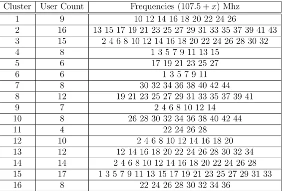
A simulation example of frequency allocation of this algorithm is shown in Table 3.1. It can be concluded that users in the same cycles of 5/9, 6/10, 7/11, and 8/12 shown in Figure 3.3 do not receive colliding frequencies. This indicates that the frequencies allocated are logical. However, this does not guarantee that the neighbor clusters do not get the same frequency band.

Table 3.1: Frequency Allocation by Centralized Frequency Allocation Algorithm Cluster User Count Frequencies (107.5 + x) Mhz

1 9 10 12 14 16 18 20 22 24 26 2 16 13 15 17 19 21 23 25 27 29 31 33 35 37 39 41 43 3 15 2 4 6 8 10 12 14 16 18 20 22 24 26 28 30 32 4 8 1 3 5 7 9 11 13 15 5 6 17 19 21 23 25 27 6 6 1 3 5 7 9 11 7 8 30 32 34 36 38 40 42 44 8 12 19 21 23 25 27 29 31 33 35 37 39 41 9 7 2 4 6 8 10 12 14 10 8 26 28 30 32 34 36 38 40 42 44 11 4 22 24 26 28 12 10 2 4 6 8 10 12 14 16 18 20 13 12 12 14 16 18 20 22 24 26 28 30 32 34 14 14 2 4 6 8 10 12 14 16 18 20 22 24 26 28 15 17 1 3 5 7 9 11 13 15 17 19 21 23 25 27 29 31 33 16 8 22 24 26 28 30 32 34 36

Algorithm 2 minimizes the total frequency interference until it reaches an optimum by testing feasible Π patterns for every cluster. The iterations continue

(46)

until no further optimization is possible and it reaches a local minimum.

This algorithm assumes a centralized implementation and assumes global knowl-edge of channel conditions between each pairs of nodes. This is certainly not suitable for distributed implementation, but can serve as a benchmark.

3.3 Mixed Integer Quadratic Frequency

Alloca-tion

Another suitable benchmark approach is to use mixed integer linear programming MIQP to obtain a global solution that minimizes the total interference level in the network. Similar to Simulated Annealing Algorithm, the minimization of the total interference level will increase the system performance and this will force a frequency allocation scheme where neighbor clusters assign different frequency bands to each other. The MIQP algorithm works on the basis of minimizing Eq (3.2) for every user pair i, j and every frequency f between fmin and fmax.

The global objective is hence to minimize the cost of interference. Equation (3.5) shows this objective. It takes in consideration of neighbor clusters that are stored in the array parameter xxij. If the clusters are not one hop neighbors, then it

is assumed that they are far away and the interference is neglected. (Later on we will show that in case of when little amount of frequencies are allocated, xxij

clusterhead neighbor parameter has to take in consideration of two-hops instead of one hop neighbors). The wij is a SNR weight parameter. The stronger SNR

value between the users i and j, the more interference they will cause to each other. hif is the output binary variable indicating whether the frequency f is

allocated to cluster i. The sideband coefficient is β1 = 10−2.5 and the second

(47)

min h ( X i∈C P j∈C P f ∈Fxxijwij[hifhjf +β1(hifhjf +1+ hifhjf −1) (3.5) +β2(hifhjf +2+ hifhjf −2)]) X f ∈F hif = X n∈V xni, ∀i ∈ C (3.6) (hif + hif +1) ≤ 1, ∀i ∈ C, f ∈ F (3.7)

There are two main constraints. First of all, the number of frequencies assigned should be to the sum of the cluster members shown in Equation 3.6. Secondly, the assigned frequencies to a cluster should have at least one band in between shown in Equation 3.7.

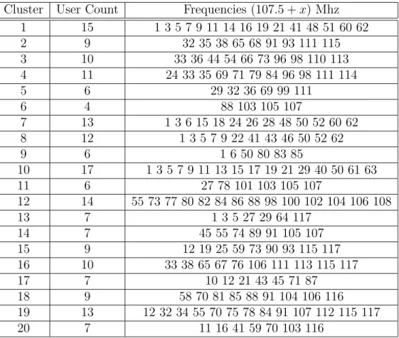
Table 3.2: Frequency Allocation by MIQP-Based Solution Cluster User Count Frequencies (107.5 + x) Mhz

1 15 1 3 5 7 9 11 14 16 19 21 41 48 51 60 62 2 9 32 35 38 65 68 91 93 111 115 3 10 33 36 44 54 66 73 96 98 110 113 4 11 24 33 35 69 71 79 84 96 98 111 114 5 6 29 32 36 69 99 111 6 4 88 103 105 107 7 13 1 3 6 15 18 24 26 28 48 50 52 60 62 8 12 1 3 5 7 9 22 41 43 46 50 52 62 9 6 1 6 50 80 83 85 10 17 1 3 5 7 9 11 13 15 17 19 21 29 40 50 61 63 11 6 27 78 101 103 105 107 12 14 55 73 77 80 82 84 86 88 98 100 102 104 106 108 13 7 1 3 5 27 29 64 117 14 7 45 55 74 89 91 105 107 15 9 12 19 25 59 73 90 93 115 117 16 10 33 38 65 67 76 106 111 113 115 117 17 7 10 12 21 43 45 71 87 18 9 58 70 81 85 88 91 104 106 116 19 13 12 32 34 55 70 75 78 84 91 107 112 115 117 20 7 11 16 41 59 70 103 116

(48)

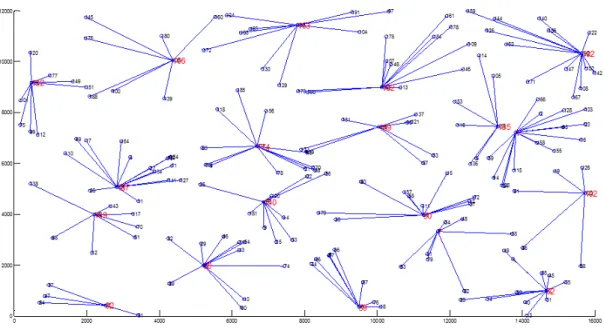
A constraint of assigning different frequencies to neighbor clusters was initially set, however it was removed latter, as the amount of frequencies have become insufficient in certain topologies when a lot of frequency bands were set per cluster. A similar table of the assigned frequencies are shown in Table 3.2. The assigned clusters can be compared with the topology assigned for these frequency sets in Figure 3.4. It is visible that same frequencies are not assigned to neighbor clusters. In fact, all first coefficient and second coefficient sidebands are avoided completely. This shows that this algorithm can be used as benchmark instead. Performance analysis will be shown in the traffic simulation chapter.

(49)

3.4 Distributed Frequency Allocation Algorithm

The distributed frequency allocation algorithm works on a marking process principle. Initially, all the clusterheads are colored white and have available frequency set Πc = Π. In the first phase, the initiator node is colored black

and allocates itself a set of channels π1 (Lines 2-3). The channel set π1 and

the sideband channel set π₁0 are removed from the available set of its neighbor clusterheads (Line 5); neighbor clusterheads cannot use these and adjacent (sideband) channels. In the second phase, clusterheads that have received a frequency set, marked black, checks whether they have a white neighbor -an unassigned clusterhead neighbor- that has not received a channel set (Line 10). The available channel set Πi for every white cluster i gets updated (Line 14).

A clusterhead allocates itself a set of frequency bands from its available set (Line 11). The available set gets re-updated by including side channels if there are insufficient available channels (Line 26). In a protocol implementation each CH can observe the control channels, and once one of its neighbors perform an allocation, it can start its own frequency allocation based on the allocation of neighbor CHs.

The proposed allocation algorithm is much simpler than the benchmark solution, as it does not assume full channel information, and only assumes CH neighbor information instead.

(50)

Algorithm 3 : Distributed Frequency Allocation Algorithm (DFA) 1: Initialize Π = {1, ..., Nf}, W = CH, B = ∅, πc= 0 ∀c = CH, Πc= Π ∀c = CH First Phase: 2: B = B ∪ 1 , W = W \ 1 3: allocate π1 ⊆ Π1 s.t. |π1| = N1 4: for ∀c s.t. a1c = ac1= 1 do 5: update Πc= Πc− π1− π 0 1 6: end for Second Phase: 7: while ∃i ∈ W do 8: for ∀i ∈ W do 9: if |Πi| ≥ Ni then 10: if ∃c ∈ B s.t. aic = aci = 1 then 11: allocate πi ⊆ Πi s.t. |πi| = Ni 12: B = B ∪ i , W = W \ i 13: else 14: for ∀c ∈ CH s.t aic = aci = 1 do 15: update Πc= Πc− πi− π 00 i 16: end for 17: if |Πi| ≥ Ni then 18: allocate πi ⊆ Πi s.t. |πi| = Ni 19: B = B ∪ i , W = W \ i 20: else

21: allocate πi ⊆ min Πused s.t. |πi| = Ni

22: end if 23: end if 24: end if 25: for ∀c ∈ CH s.t aic = aci = 1 do 26: update Πi = Πi− πc− π 0 c 27: end for 28: end for 29: end while

(51)

3.5 Frequency Allocation Performance Analysis

This section explores the performance of the frequency allocation algorithms. A detailed analysis will be further put in traffic simulation results. An important notion is that the first algorithm was based on all traffic users communicating at the same time. In that case, interference is unavoidable. However, in a military application, the amount of users communicating varies. Therefore a random traffic generation will be a good way of observing the possible interference effects. The other aspect is that the system uses TDMA. This means that the collision of two same frequencies is even lower. In other words, even if the two neighbors get the same frequency, they may never use the same frequency at the same time. This effect will be studied in the continuation of the research. This section will compare the CFA (Centralized Frequency Algorithm) to DFA (Distributed Frquency Algorithm).

3.5.1 Simulation Parameters

The algorithms were compared using the parameters shown in Tabke 3.3’. A network, consisting of 192 members are allocated with 117 different channels. At least 75 channels are assigned to more than one user. The highest frequency level will be later on changed to 188 to compare the effects of using few/a lot frequencies in traffic analysis.

Table 3.3: Simulation Parametersi for Frequency Allocation Algorithms

Parameter Description Value

fmin Lowest Frequency Level 108 Mhz

fmax Highest Frequency Level 225 Mhz

W Frequency Bandwdith 1 Mhz

N0 Noise Spectral Density -173.5 dBm

N Radio Unit Count 192

P Radio Transmission Power 10-50 Watt

Imax Cluster Count 20

Area km2 _{12x16 km}

(52)

3.5.2 Results

The algorithms were compared by searching for the worst user exposed to the highest interference level in the scenario where all users were transmitting at the same time. This would give the result for the interference to noise ratio. The noise is static and is known to be N0W . The interference is expressed

as I and the aim is to see whether the interference to noise ratio I/N0W is

similar to each other for the worst case users. The lower the ratio the better the situation. Figure 3.5 shows the ten different topology cases for the interference to noise ratio. CFA represents the centralized frequency allocation algorithm, MIQP is the solution obtained by mixed integer quadratic programming and DFA is Distributed Frequnecy Algorithm.

Figure 3.5: Frequency Algorithm Test

The results show that both centralized and MIQP frequency allocation results show similar results in providing the least interference for the worst case user. When the centralized frequency algorithm searches for a solution minimizing interference of the neighborhood clusters, it automatically decreases the

(53)

inter-ference of the worst case user. The results of the distributed clustering algorithm naturally gives a higher worst case interference levels. Nevertheless, it is sufficient to approve the expecetations of a lower interference level compared to a static frequency allocation. It has been seen that the levels of interference to noise ratio can raise by a factor varying from 300 to 9000 when frequency allocation is not applied and thus the benchmark and proposed dsitributed algorithms can be considered to be a positive result for minimizing the interference levels. The implementation of the frequency algorithms will be further discussed in the traffic simulation results.

(54)

4. ROUTING AND TRAFFIC

In the previous chapters, the clustering and frequency allocation formulations and algorithms were introduced. In this chapter, the proposed algorithms will be tested in a simulated environment created by MATLAB. In terms of application level, the various routing algorithms will be discussed and the latencies of the end-to-end communication will be analyzed for the different proposed scenarios.

4.1 Routing

Routing is the process of selecting the paths in a network. Packets are forwarded from source to destination via choosing the next hops known as the intermediate nodes. The routing algorithms for wireless networks can be tricky when nodes are mobile that connect in a dynamic manner. During the process of communication, The mobile unit can move geographically and when it goes out of range, the clustering algorithm has to recalculate its infrastructure and routing paths once again. However, this thesis focuses on a static case, and nodes are considered to be stationary throughout the simulation process. For this reason, the Dijkistra’s shortest path routing algorithm [29] is sufficient to be the routing algorithm for the traffic simulations. Dijkistra Algorithm solves the shortest path problem by assessing non-negative edge path costs, producing a shortest path tree. This table-driven algorithm is assumed to be global in our system since the infrastructure of the clustering scheme is fully connected. The cost function of the Dijkistra Algorithm is given in Equation ( 4.1). Based on the ASELSAN radio communication networks, a connection is accepted when the signal to noise ratio SN R is above 17dB. Then if there is a connection the cost of transmission is Costij = 1/SN Rij. Otherwise the cost is accepted as Costij = ∞.

(55)

Costij =    1/SN Rij, SN Rij ≥ 17dB ∞, SN Rij < 17dB. (4.1)

The cost (4.1) aims to make the source packets reach the destination with the minimum hops. Packet loss between the user i and user j does not occur unless the transmission signal to noise ratio is below 7dB. The higher the SN R the more packets can be sent simultaneously, and by Shannon’s capacity theorem there is a reciprocality between the cost and the SN R levels of the user i and user j.

Figure 4.1: Three Routing Methods in Clustering

Additionally, there are several ways the routing can occur in a clustering network. The three types shown in Figure 4.1 are the most popular routing procedures in a clustering environment. The Type 1 routing method occurs by making the clusterheads the main routers of the system. Only the clusterhead can route information to the destination node. All inter-cluster and intra-cluster communication occurs through clusterheads. The source node has to send the information to the clusterhead in order to make a successful transmission. In Type 2 routing case, intra-cluster messages are allowed. Members inside a cluster can directly send information to each other without loading the clusterhead. The Type 3 routing option is to use gateways. This can be achieved by using inter-cluster communication where inter-clusterheads that have a sufficient connection with a cluster member outside of its cluster can send information directly to those members outside of their cluster. This decreases the hop count and can be useful in unloading the traffic in the network more quickly. We have found from the simulations that Type2 routing is the most favourable in most of the cases in our system model and Type 1 is the least unfavourable (Results are shown in Section V). The delay performance is decreased by 66% in Type 1 routing. However,

(56)

ASELSAN has indicated that Type 1 routing should be used, as their systems intend on using clustering to decrease overheads, and members will be able to transmit information only via their clusterheads. Unfortunately, this results in certain traffic, such as video to cause congestion.

Figure 4.2: Network Traffic Example

4.2 Network Traffic

A traffic has been applied to our proposed communication system using clustering and frequency algorithms. The Military Radio Communication Systems use three main data types in their communication. These are Voice, Video and Command&Control messages. Command & Control and Voice messages have a high sensitivity towards delay and video communication requires a good amount of bandwidth to be efficient. These traffic types are generated randomly by random users between the transmitter and receiver. This requires a proper planning. An example of the network traffic is shown in Figure 4.2. The lines represent the routing and the intermediate nodes of the source-destination pairs. The red paths are command&control traffic type, the blue paths show the voice traffic type and the green path shows the video path. The source destinations are written in blue. The destination nodes are labeled as black.

Frequency allocation and clustering in frequency hopping AD HOC networks

TABLE OF CONTENTS

LIST OF FIGURES

LIST OF TABLES

List of Symbols

1. INTRODUCTION

1.1

Radio Communication Systems

1.2

Military Radio Communication Systems

1.3

Clustering

1.4