Macroeconomic factors and the arbitrage pricing model for the turkish stock market

MACROECONOMIC FACTORS AND THE ARBITRAGE

PRICING MODEL FOR THE TURKISH STOCK MARKET

HALE NOYAN ĠNAN

108664001

ĠSTANBUL BĠLGĠ ÜNĠVERSĠTESĠ

SOSYAL BĠLĠMLER ENSTĠTÜSÜ

ULUSLARARASI FĠNANS YÜKSEK LĠSANS PROGRAMI

TEZ DANIġMANI: OKAN AYBAR

2011

MACROECONOMIC FACTORS AND THE ARBITRAGE

PRICING MODEL FOR THE TURKISH STOCK MARKET

MAKROEKONOMĠK FAKTÖRLERĠN TÜRK HĠSSE

SENEDĠ PĠYASASINDA ARBĠTRAJ FĠYATLAMA MODELĠ

ĠLE ANALĠZĠ

HALE NOYAN ĠNAN

108664001

Okan AYBAR

: ...

Prof. Dr. Oral ERDOĞAN : ...

Kenan TATA

: ...

Tezin Onaylandığı Tarih

: ...

Toplam Sayfa Sayısı

: 73

Anahtar Kelimeler (Türkçe) Anahtar Kelimeler (Ġngilizce)

1) Hisse Senedi Getirileri

1) Stock Returns

2) Risk

2) Risk

3) Arbitraj Fiyatlama Modeli 3) Arbitrage Pricing Model

4) Makro Ekonomik Faktörler 4) Macroeconomic Factors

5) Finansal Valık Fiyatlama 5) Capital Asset Pricing

ABSTRACT

This study aims to provide evidence on macroeconomic factors which are

believed to affect stock returns of the companies listed in the ISE-30, using

the Arbitrage Pricing Model. The sensitivity of stock returns to

macroeconomic variables and explanatory power of these variables on stock

returns were investigated employing the monthly stock returns of thirteen

companies which were continuously traded within the ISE-30 index

between January 1999 and December 2009.

Factors expected to affect stock returns are assumed to be namely; the

foreign exchange rates, capacity utilization ratios, Treasury bill yields,

ISE-100 index return, money supply, industrial production, gross domestic

product, gold prices and current account deficit.

Findings suggest that the ISE-100 index return is the only variable that is

effective on the stock returns of companies. So it would be claimed that as

the model constructed in this study does not work for the sample of thirteen companies’ returns, it probably would not be valid for the stock returns of ISE-100 listed companies as a whole. Thus, this study is reduced and

bounded by the CAPM; it is no longer an Arbitrage Pricing Model. For

further research studies, a different set of macroeconomic variables and

longer time horizon on stock returns may be instructive in identifying a

ÖZET

Bu çalıĢma IMKB-30’da iĢlem gören hisse senedi getirilerini etkilediği düĢünülen makroekonomik faktörlerin etkisini Arbitraj Fiyatlama Modelini kullanarak açıklamaya çalıĢmaktadır.

Hisse senedi getirilerinin makroekonomik faktörlere karĢı duyarlılığı ve getirilerdeki değiĢimi açıklama gücü, Ocak 1999- Aralık 2009 döneminde sürekli olarak IMKB-30’da iĢlem gören 13 firmanın aylık hisse senedi getirileri kullanılarak açıklanmaya çalıĢılmıĢtır.

Hisse senedi getirilerini etkilediği düĢünülen makroekonomik değiĢkenler olarak döviz kuru, kapasite kullanım oranı, hazine bonosu faiz oranı, IMKB-100 endeks getirisi, para arzı, sanayi üretim endeksi, GSYĠH, altın fiyatları ve cari iĢlemler açığı kullanılmıĢtır.

Bulgular sonucunda, IMKB-100 endeksindeki değiĢimin bu firmaların hisse senedi getirilerinde etkili tek faktör olduğu tespit edilmiĢtir. Bu çalıĢmada oluĢturulan model söz konusu 13 firmada çalıĢmıyor ise, muhtemelen

IMKB–100 de yer alan firmalar içinde çalıĢmayacaktır.

Bu nedenle çalıĢmada bir Arbitraj Fiyatlama Modeli oluĢturulamamıĢ, çalıĢma CAPM ile sınırlı kalmıĢtır. Böylece ileri araĢtırma çalıĢmaları için farklı bir makroekonomik değiĢkenler kümesi ve daha fazla hisse senedi getirisinin, daha uzun bir zaman periyodunda incelenmesi hisse senedi

getirileri ve makroekonomik değiĢkenler arasındaki iliĢkiyi daha net açıklayabilecektir.

ACKNOWDLEDGEMENTS

I would like to thank my advisor, Okan Aybar, for his ideas, support and the

encouragement he gave me throughout the preparation of this thesis.

I would also like to thank Prof.Dr.Oral Erdogan, the director of MSc in

International Finance, for his method of approach and for helping me on

understanding the financial theories which offered me so much inspiration

and thought.

Finally, I would like to thank all of my family, all of my instructors and

friends for supporting me in the postgraduate work; without their support,

this study could not have been done.

My mother, my father, my husband and, especially, my sister, Ebru Noyan

TABLE OF CONTENTS

3. METHODOLOGY AND DATA ... 42

3.1 Methodology ... 43

3.2 Data ... 46

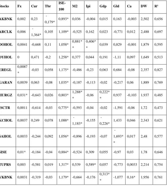
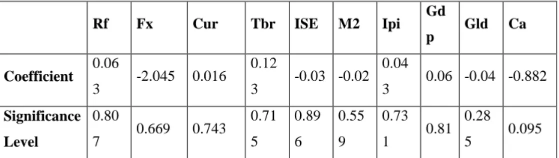
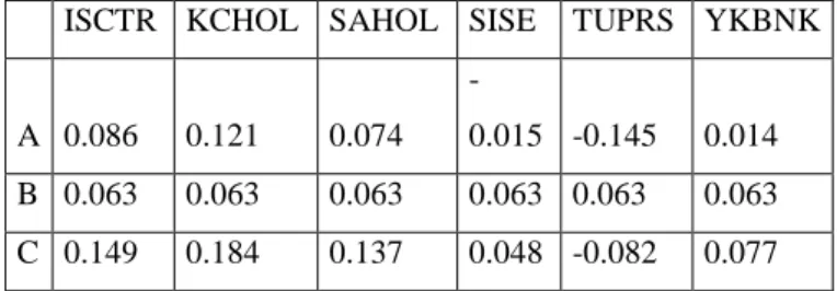
4. FINDINGS ... 54

5. CONCLUSION ... 64

LIST OF FIGURES

Figure 1: Markowitz Portfolio Selection ………. 15 Figure 2: Capital Market Line ………. 17

LIST OF TABLES

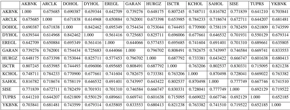
Table 1: Macroeconomic Variables and Previous Studies ……... 47 Table 2: ISE-National 30 Companies Codes………... 48 Table 3: Regression Equation Results………. 54 Table 4: Results of the Cross Sectional Regression Analysis ………... 59 Table 5: Contribution of Risk Premiums to Expected Return (1) ….. 60 Table 6: Contribution of Risk Premiums to Expected Return (2) ….. 61 Table 7: Estimation of Excess Expected Returns to Stocks (1) ..……. 61 Table 8: Estimation of Excess Expected Returns to Stocks (2) ..……. 61 Table 9: Correlation Matrices of ISE-National 30 Companies ...…… 63

LIST OF ABBREVIATIONS

MPT : Modern Portfolio Theory

CAPM : Capital Asset Pricing Model

APM : Arbitrage Pricing Model

RFR : Risk Free Interest Rate

I-CAPM : International Capital Asset Pricing Model

ISE : Istanbul Stock Exchange

GNP : Gross National Product

FA : Factor Analysis

PCA : Principal Component Analysis

AKBNK : Akbank

ARCLK : Arçelik

DOHOL : Doğan Holding

DYHOL : Doğan Yayin Holding

EREGL : Ereğli Demir Çelik

GARAN : Garanti Bankası

HURGZ : Hürriyet Gazetecilik

ISCTR : ĠĢ Bankası C

SISE : ġiĢecam

TUPRS : TüpraĢ

YKBNK : Yapi Kredi Bankasi

FX : Foreign Exchange Rate

CUR : Capacity Utilization Ratio

TBR : Treasury Bill Rate

ISE 100 : Ise 100 Index

M2 : Money Supply

IPI : Industrial Production Index

GDP : Gross Domestic Product

1. INTRODUCTION

Finance theory plays significant role on how financial decisions are taken in

risky stock markets. In this context, the risk – return relationship has gained

prominence. The subjects of minimizing risk and maximizing return have

been investigated. The portfolio management involves decisions on the type

of assets in a portfolio, given the goals of the portfolio owner and changes in

economic conditions. Selection has some constraints, most typically the

expected return on the portfolio and the risk related with this return.

In literature, two main theories are instructive for investors. The traditional

theory, assumed that risk could be reduced by raising the number of

financial assets in a portfolio, without taking into consideration the

relationship between the returns of the financial assets.

The second was modern portfolio theory. Modern Portfolio Theory was widely recognized in 1952 with publication of Harry Markowitz’s article “Portfolio Selection” in the Journal of Finance. In this paper, Markowitz provided a definition of risk and return as the mean and variation of the

outcome of an investment (Markowitz, 1952).

The variation of return between financial assets can be explained by the

Capital Asset Pricing Model and the Arbitrage Pricing Model.

The Capital Asset Pricing Model describes the relationship between risk and

expected return, which is used in pricing risky securities.

expected return of a theoretical risk-free asset. The shortcomings of the

capital asset pricing model directed researchers towards new model

findings.

In this sense, a new model after CAPM is the Arbitrage Pricing Model,

which was developed by Stephen Ross in 1976. The model implies that the

expected return of a financial asset can be explained by various

macroeconomic factors, where the sensitivity to each factor is specified by

the specific beta coefficient. Chen, Roll and Ross (1986) sought to identify a

number of macroeconomic factors (surprises in inflation, surprises in GNP

through an industrial production index, changes in default premium

corporate bonds, surprise shifts in the yield curve) as significant in

explaining the returns of securities.

As such, the main objective of this research is to investigate the relationship

between macroeconomic factors and the Arbitrage Pricing Model in the

2. LITERATURE REVIEW

“Portfolio Selection”, was published by Harry Markowitz in the Journal of Finance, can be considered as first paper in the history of Modern Portfolio

Theory (MPT).

The work of Markowitz (1952) proposes how rational investors would use

diversification to optimize their portfolios. The model treats asset returns as

a random variable and assumes the portfolio as a weighted combination of

assets. Moreover, the portfolio return is a random variable and has an

expected value and a variance. According to MPT, risk is the standard

deviation of the return.

Markowitz’s study on portfolio selection can be accepted as a revolution in the theory of finance, and a light for the foundation for capital market theory

(Jensen, 1972).

Markowitz mainly concentrated on the special case in which investor

preferences can be defined over the mean and variance of probability

distribution of single period returns.

The major studies are concentrated on two arguments. The first was Tobin’s

(1958) study which uses the assumptions and foundations of MPT, drawing

implications regarding demand for cash balances, and second concerns the

general equilibrium models of asset prices, derived by Treynor (1961),

Sharpe (1964), Linter (1965-1, 1965-2), Mossin (1969), Fama (1968).

investors should behave. The MPT focuses on how investors perform

diversification to optimize their portfolios. Each of the models, such as

Treynor (1961), Sharpe (1964), Linter (1965), Mossin (1969) and Fama

(1968) represents an investigation of the Markowitz Model for the

equilibrium structure of asset prices. It is important here to understand that

the MPT is not based on validity or lack of the capital market theory.

The models involve the following assumptions:

1) All investors can lend or barrow money at the risk-free rate of

return.

2) All investors have identical probability distributions for future

rates of return; they have homogenous expectations with respect

to three inputs of the portfolio model: the expected return, the

variance of returns and the correlation matrix.

3) All investors have access to the same information to generate an

efficient frontier.

4) All investors are single period expected utility of terminal wealth

maximizers.

5) There are no transaction costs.

6) There is no personal income taxation on returns; investors are

indifferent between capital gains and dividends

8) All investors have identical subjective estimates of the means,

variances and covariance of return among all assets.

9) All assets are infinitely divisible and liquid, indicating that

fractional shares can be purchased and stocks may be infinitely

divisible.

10) There is no taxation.

11) There is no inflation.

12) All investors are price takers.

13) Capital markets are in equilibrium (Sharpe, Alexander, 1990).

The main objective of portfolio management is the selection of assets which

maximize the return and minimize the risk for investors.

One of the most popular approaches to portfolio selection is diversification

of assets, such that risk is spread over a mixture of asset types. Each asset

exhibits a different risk return performance.

As a result, investors tend to furnish their portfolios with assets which either

lack of a strong correlation between them, or bear a negative correlation.

Thus in this section, the expected return – risk concepts and capital asset pricing models are covered. The Expected Return (“E (R)”) is the mean value of the probability distribution of possible returns.

Variance (ζ ²) measures the dispersion of a return distribution. It is the sum of the squares of the deviations (from the mean) of the returns, divided by n.

The value will always be greater than or equal to 0 with larger values

corresponding to data that is more spread out.

The standard deviation (ζ) is the statistical measure of degree to which an individual value in probability distribution tends to vary from the mean of

distribution (Davis, 2001).

The objective of the investor is to maximize the portfolio’s expected return

with an acceptable level of risk. The Markowitz model is a single – period

model and it is assumed that investors form a portfolio at the beginning of

the period.

The assumption of a single time period allows risk to be measured by the variance (or standard deviation) of the portfolio’s return.

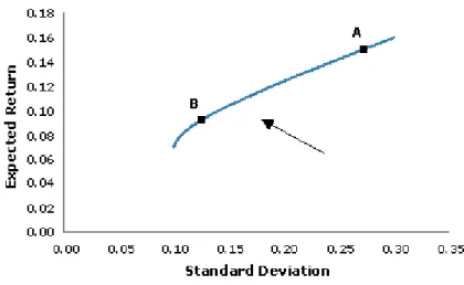
These, as in Figure 1, investors are seeking to the upper left hand side of the

graph.

Figure 1 Markowitz Portfolio Selections (Source: Davis, 2001)

The curve is known as efficient frontier. According to the Markowitz model,

risk. Risk takers will choose point A, which the risk averse investor would

be more likely to choose portfolio B.

Building on Markowitz framework, William Sharpe (1964), John Linter

(1965) and Jan Mossin (1966) independently developed a model known as

the Capital Asset Pricing Model (CAPM).

The CAPM can be considered as the birth of asset pricing theory (Nobel

prize for Sharpe in 1990). This model assumes that investors use Markowitz

work in forming their portfolios. As a further step, this model accepts that

there is a risk free asset that has a certain return, which is riskless or

risk-free.

Here, the risk free rate is the current interest rate on a bond, for which there

is no risk of default, in the absence of inflation. With a risk free asset, the

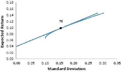
efficient frontier is no longer the best return that investors can achieve. The

capital market line shows the combinations of risk free assets and a risky

portfolio. Investors choose portfolios along this line, with the efficient

frontier being the tangent. As CAPM assumptions indicate that investors

combine the market portfolio and the risk-free asset, the only risk that

investors are paid for holding is the risk associated with the market

Figure 2 Capital Market Line (Source: Davis, 2001).

E (rp) = Rf +

E(rm)-rf σm *σp

E (rp) : Expected return of the portfolio

Rf : Expected return of the risk free asset

E (rm) : Expected return of the market portfolio

ζm : Standard deviation of the market portfolio ζ p : Standard deviation of the portfolio

The gradient of the capital market line represents the price of risk in market

and can be explained by the formula as follows:

[E (Rm – Rf)] / ζm

The ratio of covariance between expected return of the market and the

 m) accepted as a risk and is used for asset pricing. The expected return of an asset will be shown as:

E (Rp) = Xi x E (Ri) + (1- Xi) x E (Rm)

E (Rp) : Expected return of portfolio

E (Ri) : Expected return of asset i

Xi : Weight of asset i in total investment

E (Rm): Expected return of market portfolio

The risk of portfolio is as follows:

ζ p = [Xi² x δi² + (1 – Xi²) x ζm² + 2 x Xi x (1 – Xi) x ζim]1/2 ζ p : Standard deviation of the portfolio

ζi² : Variance of asset i

ζm² : Variance of the market portfolio

ζim : Covariance asset i and market portfolio

As a result, the Capital Asset Pricing equation will be

E (Ri) = Rf + [ E (Rm) – Rf) / ζim²) x ζim

Under the CAPM, the beta coefficient represents the part of asset risk that

can not be diversified away, and represents the risk that investors are

compensated for bearing. It represents the systematic risk. So the equation

βi =

σim

σm2

βp =



βp : Beta coefficient of portfolio βi : Beta coefficient of asset I Xi : Weight of asset i in portfolio

The representation of the CAPM equation is:

E (Ri) = Rf + [E (Rm) – Rf) x βi

The CAPM equation states that the expected return of any risky asset is a

linear function of its tendency to changewith the market portfolio when the

beta is included as an explanatory variable.

The assumptions of the CAPM can be summarized as follows:

All investors

1) Aim to maximize economic utility.

2) Are rational and risk averse.

3) Are price takers, i.e. they can not influence the prices.

4) May lend or borrow to an unlimited extent at the risk-free rate of

interest.

5) Are not subject to transaction fees or taxes

7) May access information which is available to all investors at the

same time

8) Operate in perfectly competitive markets.

Like all other models, the CAPM has some shortcomings. The CAPM

assumes that asset returns are normally distributed and that investors have a

quadratic utility function; in practice, equity returns are not normally

distributed.

Another important assumption of the CAPM is the risk concept. This

assumes that the variance of returns is an adequate measurement of risk.

However, other risk measures will reflect investor preferences more

adequately. In finance, investors tend to perceive risk as a probability of

losing. As a result, risk in financial investments is not limited to the variance

itself. The CAPM accepts the assumption of homogenous expectations. In

practice, there is heterogeneity of information among investors.

Behavioral finance examines investors’ different probability beliefs. The CAPM assumes that investors’ probability beliefs match the true distribution of returns.

Kent Daniel, David Hirshleifer and Avanidhor Subrahmanyann (2001)

performed studies on behavioral finance it uses physiological assumptions

to provide alternatives to the CAPM, such as the over confidence based on

The CAPM does not have an explanation for the variation in stock returns.

Empirical studies have found that low beta stocks may offer higher returns

than the CAPM would predict.

Black, Jensen, Scholes (1969) published a paper where they found that if the

efficient market hypothesis was supported by the CAPM would be wrong or

irrational. The opposite is also true i.e. if the CAPM was supported, the

Efficient Market Hypothesis would be wrong. In a paper known in literature as Roll’s critique, Roll (1977) highlighted that the CAPM may not be empirically testable. The market portfolio should include all types of assets

that are held by investors (such as art works, real estate, and human capital).

In practice, such a portfolio is unobservable. As a result, people substitute a

stock index as a proxy for the true market portfolio. Unfortunately, in

empirical studies it was shown that this substitution may lead to false

inferences as to the validity of CAPM.

The CAPM assumes that investors will optimize their assets in one

portfolio. The Maslowian portfolio theory stated that investors tend to hold

fragmented portfolios. Investors may hold one portfolio for each goal.

The validity of the CAPM was researched by Linter (1971), Sharpe and

Cooper (1972), Mayers (1976), Merton (1973), Goredes (1976), Rubinstein

(1976), Elton and Gruber (1978) and Breeden, Gibbons and Lizenberger

(1989).

Based on the Capital Asset Pricing Model (CAPM) assumptions, new

models to the CAPM are the Zero – Beta CAPM, the Inter temporal CAPM,

the Multi-Beta CAPM, the consumption based CAPM and the international

CAPM.

The model developed by Fisher Black (1972) drops the assumption,

contained in the CAPM that investors may borrow and lend at the risk-free

rate. In fact, the Zero – Beta CAPM treats all assets as risky. It is assumed

that there is no such thing as a risk-free asset.

Rather than relying on the existence of risk-free assets, all that this required

is the existence of an asset whose return is not correlated with the market

portfolio – in other words, a Zero-Beta portfolio (Black, 1972).

It argues that inflation reduces the purchasing power in risk-free bonds and,

as such, consists of purchasing power risk. The main assumption is that

investors cannot borrow and lend at the same rate of interest. The Capital

Asset Pricing Model is static; in other words, a single period model. It

ignores the multi period nature of participation in capital markets.

Merton’s (1973) Inter temporal Capital Asset Pricing Model (CAPM) captures the multi – period aspect of financial markets. In the Inter temporal

model, investors act to maximize the expected utility of lifetime

consumption and can trade continuously in time.

Moreover, it is stated that explicit demand functions for assets are derived

and it is shown that in contrast with the one period model, current demand is

The CAPM is useful in classifying risks relevant to returns as systematic

risk. In order to state systematic risk more clearly, the standard CAPM

should be developed in such a manner that it can measure the sensitivity to

different risk sources. At the end of this development process, the Multi –

Beta CAPM is introduced.

The Multi – Beta CAPM examines how different sources of risk affect stock

returns. While the CAPM claims that market risk is to be priced, the Multi –

Beta CAPM has proven that risks other the market should be considered

(Merton, 1973).

Merton suggested that some factors such as uncertainty over wages, the

prices of some important consumer goods and increases in the risks of some

asset groups could be considered as sources of risk (Bodie, Kane and

Marcus, 1999).

The multi – Beta CAPM equation can be set out as below (Elton and

Gruber, 1997).

Rpt – RFR = p +  p (Rmt – RFR) + p’ (Rm’t – RFR) + ept Rpt : Expected return of portfolio

RFR : Risk – free interest rate

αp : Constant term

βp : Sensitivity of the portfolio to the stock index Rm : Return of the stock index

Rm’ : Return of the bond index ep : Error term

The Multi – Beta CAPM considers a wide range of risk sources.

Another alternative to the CAPM is the consumption – Based Capital Asset

Pricing Model.

Breeden (1979) provides a logical extension of the previous CAPM. Based on “diminishing marginal utility of consumption”, there will be high demand for securities which offer high returns when the aggregate

consumption is low, bidding up their prices. In contrast, stocks that change

positively with aggregate consumption will require higher expected returns.

Breeden derived the Consumption – Based Capital Asset Pricing Model:

E (Rj) = Rf + βjc [E(Rm)-Rf]

In this model, the market beta coefficient is replaced by a consumption – based Beta coefficient. βjc measures the sensitivity of return asset to changes in aggregate consumption. The main result of the Consumption

based asset pricing model is that expected returns should be a linear

function of consumption betas (Davis, 2001).

Empirical tests have not supported the predictions set out in the

consumption based capital asset pricing model (Breeden, Gibbons and

Litzen Berger, 1989).

Literature covering the International CAPM shows that when purchasing

power parity does not hold, the asset pricing model includes exchange risk

factors. The exchange rate risk factor, as in the International CAPM, is a

hedging factor due to predictability of future real exchange rates (Tat, Ng,

2001).

The International capital pricing model treats global market risk and foreign

exchange rate risk under the assumption of time variation in all prices of

risk. The model takes inflation risk into account. Thus, in I – CAPM

assumptions, there are restrictions on international investments, such that it

is not possible to determine prices independently. Another assumption of

Solnik (1974) is that international investors have different preferences and,

accordingly, different satisfaction levels. The equation for the International

CAPM developed by Solnik (1974) and Merton (1973) is as follows:

E (Ri) = Rfi + (E (Rwm) – Rfw) x βwi

E (Rwm) = Expected return of global market

Rfi = Expected return of domestic asset i

Rfw = Average international risk-free interest rate

βwi = Systematic risk of asset i which reflects the covariance of world market portfolio and asset i

The Multi beta – forms International Capital Asset Pricing Model is

developed for the Arbitrage Pricing Model.

Arbitrage Pricing Model. In this part of study, we first explain the arbitrage

concept and then examine the arbitrage pricing model in detail.

Arbitrage is the practice of taking advantage of a state of imbalance between

two (or possible) markets and thereby enjoying a risk-free profit. In the APT

context, arbitrage consists of trading in two assets, at least one of which is

mispriced. The arbitrageur sells the asset, which is relatively expensive, and

uses the proceeds to buy one which is relatively cheap

The literature on asset pricing models has taken on a new lease of life since

the emergence of Arbitrage Pricing Model (APM). The APM was

formulated by Ross (1976) as an alternative theory to the renowned Capital

Asset Pricing Model (CAPM) proposed by Sharp (1964), Linter (1965) and

Mossin (1966).

The Arbitrage Pricing Model assumes that the expected return of a financial

asset can be modeled as a linear function of various macroeconomic factors

or theoretical market indices, where sensitivity to changes in each factor is

represented by a factor specific beta coefficient.

Focusing on capital asset returns governed by a factor structure, the

Arbitrage Pricing Model is a one – period model, in which the preclusion of

arbitrage over static portfolios of these assets leads to a linear relationship

between the expected return and its covariance with the factors.

The theory was initiated by the economist Stephen Ross (1976), Brown and

Mosser (1988), Otateye (1992) followed Ross’s research and many empirical researches tried different methods to test APT.

On the basis of traditional assumptions that asset markets are perfectly

competitive, frictionless and where individuals have homogenous beliefs

that random returns on assets are generated by the linear k-factor model, the

return on the ith asset can be written of the form:

Ri = Ei + bi1I1 + bi2I2 + bi3I3 + . . . + bikIk + ei ( i = 1………n)

Where:

Ri is the random rate of return on the ith asset

Ei is the expected rate of return on the ith asset

bik measures the sensitivity of the ith asset’s returns to the k factor

Ik denotes the mean zero kthfactor common to the returns of all assets

ei is a nonsystematic risk component idiosyncratic to the ith asset

mean zero and variance ζ2 Ri

With no arbitrage opportunity, it can be shown that the equilibrium expected

return on the ith asset is given of the form

Ei = λo + λ1bi1 + λ2bi2 + ………. + λkbik (2)

If there is a risk-free return E0, its return will be λo = E0. Forming a portfolio with unit systematic risk on λk (k = 1……….k) and no risk on other factors, the final form of the APM is derived as follows:

Ei is the expected return on the ith asset

E0 is the return on the riskless asset

Ek is the expected return on a portfolio that has a unitary sensitivity

to the kth factor and zero sensitivity to all other factors

bik is the sensitivity of the ith asset to the kth factor

λk = (Ek – E0) (k = 1……….k) is the risk premium associated with the corresponding risk factors; Ik.

As a result, in the event that the equilibrium prices offer no arbitrage

opportunities over the static portfolios of the assets, the expected returns on

the assets assume an approximately linear relationship to the factor loadings.

The factor loadings or betas are proportional to the covariance of the returns

with the factors (Ross, 1976). If agents maximize certain types of utility, the

linear pricing relationship is a necessary condition for equilibrium in a

market (Ross, 1976).

The APM was developed after the CAPM. The APM is very similar to the

CAPM. It states that the expected return on any security in equilibrium will

be equal to the risk free return plus a set of risk premiums. There are a

number of differences between the APM and the CAPM; the CAPM only

has one factor (excess return of the market portfolio) to explain the excess

return of asset.

The systematic risk of an asset is then stated by the correlation with this

premiums for bonds, or surprise shifts in the yield curve. The market

portfolio in itself does not capture all the sources of systematic risk. The

CAPM is an equilibrium model and derived from individual portfolio

optimization. The APM, on the other hand, is a statistical model which

seeks to capture the sources of systematic risk. The relationship between the

sources is determined by the condition of no arbitrage. In contrast to the

CAPM, the Arbitrage Pricing Model is derived from an arbitrage argument,

not a market equilibrium argument. The risk premium follows from the

factor structure of asset returns.

The arbitrage pricing model does not rely on measuring the performance of

the market. Instead, the APM directly relates the price of security to the

fundamental factors driving it. The problem with this is that the theory in

itself provides no indications of these factors are so they need to be

empirically determined. Obvious factors are economic growth and interest

rates. For companies in certain sectors, other factors are obviously relevant

as well, such as consumer spending for retailers.

Such a potentially large number of factors mean more betas need to be

calculated. There is no guarantee that all relevant factors have been

identified. It is a result of this added complexity that the arbitrage pricing

model is more widely used than the CAPM.

Roll and Ross presented methods for estimating the return generating

process and for testing whether particular factors in the return generating

process were priced in equilibrium. They found that more factors are priced

held. Roll and Ross used the maximum likelihood factor analysis to estimate

both the number of factor generating returns and factor loadings. Dhrymes,

Friend and Gültekin (1984) observed that the number of significant factors

increases with the number of stocks employed in the factor analysis and that

tests of the APM depend very much on how the stocks are grouped.

Fundamental foundation for the arbitrage pricing model is the law of one

price, which states that two identical items will sell for the same price; if

they do not, a riskless profit, could be generated by arbitrage, meaning that

an item could be purchased in a cheaper market and then sold in a more

expensive market. The arbitrage is performed simultaneously because the

price discrepancy must be taken the advantage of immediately. Otherwise, it

would likely disappear by the time of settlement.

The law of one price, as applied in the arbitrage pricing model, can be stated

as follows. It is stated that two financial instruments or portfolios - even if

they are not identical - should cost the same if their return and risk is

identical. The law of one price requires that any two financial instruments or

portfolios that have the some return – risk profile should sell for the same

price. If they do not sell for the same price, then a profit can be earned by

short-selling the security or portfolio with a lower return and by buying the

portfolio with the higher return.

The arbitrage pricing model offers on alternative to the CAPM as a method

in computing the expected return on stocks. The basis for the Arbitrage

number of factors affecting stock returns. These models can be placed into

two groups: single risk factor and multifactor models.

Ross (1976) assumes that there is a lack of arbitrage opportunities in capital

markets and accepts a linear relationship between returns and a set of

common factors (K common factors), assuming that the expected returns

will be linear functions of common weights. This assumption recommends

the use of Factor Analysis (FA) which is developed by Spearman and

Hatelling as a potential tool for the extraction of the K common factors from

the return of assets.

In the context of the APM, the assumption is that the population of a stock

return is generated by a factor model. The simplest factor model is the one

factor model:

ri = αi + βiF + εi E(εi) = 0

In the single factor model, the fundamental foundation for the arbitrage

pricing model is the law of one price, which indicates that two items will be

sold for the same price; unless they have a riskless profit could be generated

by arbitrage, which means buying the item in a cheaper market then selling

it in a more expensive market. In the event of arbitrage opportunities, the

arbitrageur is able simultaneously buy the stock on the cheaper exchange

and short-sell it on the expensive exchange for a riskless profit. This process

would then continue until the price discrepancy has disappeared. As a

demand, and therefore the price; on the other hand, short selling on the more

expensive exchange would increase supply, thereby reducing its price.

ri = αi + βiF + εi E(εi) = 0

A graph of this line is the arbitrage pricing line for the single risk factor.

In the equation of the single – factor model:

ri = αi + βiF + εi E(εi) = 0

In the single factor model, factor F is proposed to affect all stock returns, in different sensitivities. Here, the sensitivity of stock i’s return is denoted by βi. It means that stocks with low β values, will only exhibit a slight reaction as F changes; on the other hand, when βi is high, variations in F cause substantial movements in the return of stock i. In the event that the two

stocks in the portfolio have positive sensitivities to the factor, both will tend

to move in the same direction.

A second main component in the factor model is the random stock to returns

which is assumed to be uncorrelated across different stocks. There is also a term, εi, which represents the idiosyncratic return component for stock i. An important property of εi is that it is uncorrelated with factor F (the common factor in stock returns).

In the equation,

it is implied that all common variation in stock returns is generated by

movements in F. As idiosyncratic components are uncorrelated across

assets, they do not bring about co-variation in share price movements.

Numerous studies (Trzcinka 1986, Connor and Korajcyzk 1993; Geweke

and Zhou 1996; Jones2001; Merville and Xu 2001) demonstrate the

importance of one factor, shown as the market factor, which explains a

significant part of the return variation, while identifying other factors such

as industry specific factors have been attributed to the lack of formal criteria

for choosing the number of factors (Harding, 2007).

Harding (2007) showed that it is not possible to distinguish some of the

factors from the idiosyncratic noise by heuristic methods or by a random

matrix approach. In short, Harding showed that unless the period of time

over the observed portfolio is extremely long, it is not possible to identify

all factors of the economy.

As stressed, the APM begins by assuming that asset returns follow a factor

model.

A generalization of the structure identifies k factors or sources of common

variation in stock returns. Different stocks should be allowed to have

different sensitivities to different types of market wide shocks. As a result,

multifactor models can provide a better description of security returns.

ri = αi + β1i F1 + β2i F2 + ……… + βki Fk + εi E(εi) = 0

The returns of asset i depend, in a linear fashion, on k factors and

The idiosyncratic component is assumed to be uncorrelated across stocks

with all of the factors and the idiosyncratic risk is, on average, zero. The

factor can be thought of as representing news on macroeconomic factors,

financial conditions and political events. It is assumed that each stock has a

complement of factor sensitivities or factor betas, which determine the

sensitivity of the return on the stock in question is to variations in each of

the factors.

To sum up, with a large number of available assets, Ross implies that

idiosyncratic risk is diversifiable and prices of securities will be

approximately linear in their factor exposures.

As Fama (1991) highlighted, one can not expects any particular asset

pricing model to completely describe reality; however, Fama argued that the

asset pricing model is a success if it improves our understanding of security

market returns. In the light of this view, the APM is indeed a success. On

the other hand, the APM has some weakness and gaps. For instance, the

model itself does not identify what the right factors are. In addition, if it is

supposed that where the model explains the right factors, the factors can

change over time. Finally, unless the period of time over which the portfolio

covers is extremely long, it is impossible to identify all factors of the

economy; thus estimating multifactor models requires more data. The APM

would be a better model if it was related to factors more closely identifiable

and measurable sources of economic risk. If all strengths and weakness are examined and changes occur, Ross’s insight would serve as a fundamental

In addition, Connor, Chen, Ingersoll argued that if the numbers of assets are

greater than the number of factors, sound diversification would not be a

problem in security pricing.

The Arbitrage Pricing Model is based on the assumption of a linear

relationship between asset returns and a number of common factors

(Trzcinka, 1986). Asset returns are a linear function of a number of risk

factors. In this perspective, one weakness of the Arbitrage Pricing Theory is

that the model does identify the number of factors, or what the right factors

are.

Most research studies in literature concerning the Arbitrage Pricing Model

are focused on three types of factor models, which are macroeconomic,

fundamental and statistical.

The macroeconomic model identifies macroeconomic indicators as factors.

Common factors affecting returns in the market may include inflation

shocks, spreads between long and short term interest rates, yields spread

between long term corporate and treasury bills, oil prices and the rate of

GDP growth.

Chen, Roll and Ross (1986) identified these macroeconomic factors as

significant in explaining security returns:

 Surprises in inflation

 Surprises in GNP as indicated by the industrial production index

 Surprises in investor confidence due to changes in default premium in corporate bonds;

 Shifts in the yield curve.

Another model which is a fundamental factor model uses company and

industry data as factors affecting the stock returns. Here, accounting ratios of a company (such as its debt to equity ratio or fixed rate ζ average) can be combined with other relevant financial variables into a leverage risk factor.

On the other hand, as market information, such as share turnover or trading

volume can be combined with other relevant financial information and can

act as a trading activity risk factor.

Statistical factor models represent factor analysis and principal component

analysis. Factor analysis is a statistical method used to describe variability

among observed variables in terms of fewer unobserved variables called

factors. The observed variables are modeled as linear combinations of the

factors. In order to imply the factor analysis to the Arbitrage Pricing Model

at first, covariance of asset returns must be estimated; later factors are

extracted from the covariance matrix. Factor analysis offers an opportunity

for the reduction of number of variables, by combining two or more

variables into a single factor. In addition, identification of groups of inter –

related variables shows the extent to which they are related to each other

Likewise, principal component analyses are used to determine the factors,

factor’s variance explains the maximum percentage of variability in stock returns. The second factor, which is uncorrelated with the first factor,

explains most of the remaining variability. For the other factors, the same

procedure will be followed (Omron, 2005).

Factor analysis is related to principal component analysis, but not identical

to it. PCA takes into account all variability in variables; in contrast, factor

analysis estimates how much of the variability is due to common factors.

Factor analysis focuses on communality.

Roll and Ross (1980), Chen (1983) and Lehman and Modest, 1985a, 1985b)

used factor analysis. However Chamberlain and Rothschild (1983), Connor

and Korajczyk (1985, 1986) recommended Principal Component Analysis.

The Arbitrage Pricing Model was first initiated by Ross (1976a, 1976b) in a

one period model, in which returns of a capital asset are a linear function of

factor structure.

As Ross Stated, returns of a capital asset are consistent with a set of factor

structures, such as macroeconomic changes. Some macroeconomic changes

affect asset prices more, while some of them do not even affect them at all.

In literature, the theoretical question of “which economic factors have significant effects on the pricing mechanism” is sought to be solved by many empirical studies.

Chen, Roll and Ross (1986), have tested a set of economic data for US stock

return. They analyzed the effects of macroeconomic variables, term

consumption and oil prices between the periods of January 1953 –

November 1984.

They note that if industrial production, changes in risk premium, twists in

the yield curve and changes in expected inflation are highly volatile, they

are significant in explaining the expected returns.

Some other empirical studies of APM focus on the identification of a

number of risk factors that systematically explain the stock market returns

by implementing Factor Analysis Methods.

Dhrymes, Friend and Gültekin (1984) examined the techniques used in the work carried out by Roll & Ross and found that if the stocks are categorized

into groups, there will be some deviation in the results. They found some

limitations to the work carried out by Roll and Ross. In the study performed by Dhrymes, Friend and Gültekin, they found that the number of “factors” extracted increases with the number of securities in the group. At a 5%

significance level, with a group of 15 securities, they found the most “common risk” factors with a group of 30 securities. They found three “common risk factors” with a group of 45 securities and four common risk factors with a group of 60 securities and, at most, six “common risk factors” with a group of 90 securities, and they found nine common risk factors.

Their study stressed the difficulty of identifying the actual number of factors

affecting the returns.

In addition, they found that the number of “factors” increases with the number of time series observations used to estimate factor loading. Finally,

they claim that the constant term differs from risk free rate and that the error

term is not statistically equivalent to zero.

Chen (1983), using the factor analysis, tested the APM and compared it with

the CAPM. In conclusion, Chen noted that we cannot reject the APM. APM

performs better than the CAPM.

Brown and Weinstein (1983) estimated and tested the APM using the same

data as Roll and Ross (1980). The difference between Brown and

Weinstein’s study and Roll and Ross’s study was the grouping of securities

in batches of 60 instead of 30, and according to their industrial

classifications instead of alphabetical order. However, by grouping

according to industrial classification rather than alphabetical order, asset

prices will be affected by more than three factors. In short, the results

support the APM.

Sharpe examined the stock returns of 2,197 companies between 1931 and

1979 and found that the expected return of an asset can also be explained by

micro factors, in addition to market beta. The use of micro factors with

macro factors can increase the explanatory power of the model.

Poon and Taylor (1991) considered the results of Chen, Roll and Ross to

check whether the variables in that model were applicable to the UK stock

market. The economic variables used in the work carried out by Chen, Roll

and Ross were the monthly and annual growth rates of industrial production,

unanticipated inflation, risk premium, the term structure of return value and

showed that the factors put forward by Chen, Roll and Ross for the US

market do not influence share prices in the UK market. They claimed that

there may be other macroeconomic variables at work, and that Chen, Roll and Ross’s work was inadequate when it came to detecting such pricing relationships.

A research study performed by Özçam (1997) can be accepted as an example of APM testing of the Istanbul Stock Exchange. Özçam tested seven macroeconomics variables of the Turkish economy by separating

them into expected and unexpected series through regression process. A

two-step testing methodology was then implemented on these series. The

study was performed for 54 stocks over the period of January 1986 to July

1985. The result supported the APT, where beta coefficients of expected

factors were found to be significant in determining the asset return.

Yörük (2000) used ten macroeconomic variables to find the risk premium and sensitivity of stocks listed on the Istanbul Stock Exchange for the period

of February 1986 to January 1998, on a monthly basis. The period was

divided into three subs – periods, of February 1986 to January 1990,

February 1990 to January 1994 and February 1994 to January 1998. The macroeconomic variables used in Yörük’s research were the percentage change in the consumer price index, the percentage change in industrial

production, the manufacturing production index, current account balances,

the consolidated budget, the non cumulative cash balance, money supply

Altay (2001) used two different APT tests on the Istanbul Stock Exchange.

In the first test, factor analysis was used for daily returns of 121 to 265

stocks in the period of 1993 – 2000 for each year. One significant factor was

found among several factors for each year. The second test was performed

through a multivariable regression process in order to examine the

significance of macroeconomic variables on asset returns. The study found

that the beta of the Treasury bill interest rate was significant for explaining

the asset returns.

In another study, Altay (2003) derived the factor analysis process and factor

realizations for two countries, Turkey and Germany.

There are several empirical studies on the Arbitrage Pricing Model. The

number of factors affecting stock returns has proliferated; however the theoretical question of “which economic factor data sets have significant effects, and the exact number of factors” is not answered clearly.

3. METHODOLOGY AND DATA

The 1980s are the years deregulation and internalization of financial

markets in Turkey. Until 1980, the Turkish economy was a closed economy.

However, new regulations introduced on January 24, 1980, marked a sharp

break with the past economic development policies. Interest rate controls

were lifted and entry barriers into the financial system were relaxed (Denizer, Gültekin, Gültekin, 2000).

In 1981, the Capital Markets Board of Turkey (CMB), which is the

regulatory and supervisory authority in charge of securities markets in

Turkey, was set up.

The CMB has set out detailed regulations for organizing the markets and

developing capital market instruments and institutions for the past twenty

nine years in Turkey.

In 1984, Turkish residents were permitted to hold foreign currency deposits.

This process marked a step towards the opening of the capital account in

1989, which also meant that the opening increased funding options abroad,

both for the financial system and for large corporations. These reforms

clearly represented major progress towards freeing the operation of the

financial markets. By following the development of international financial

markets, in 2000, futures markets were set up on cotton contracts.

On 4 February, 2005, VOB – a Turkish derivate exchange - started

a) Currency Futures Contracts: TRY/US Dollar, TRY/Euro,

PDTRY/US Dollar, PDTRY/Euro

b) Interest Rate Futures Contract: T – Benchmark Futures.

c) Equity Index Futures Contract: TurkDEX – ISE 30 Futures,

TURKDEX – ISE 100 Futures.

d) Commodity Futures Contracts: Cotton Futures Contract,

Wheat Futures Contract, Gold Futures Contract.

3.1 Methodology

In finance theory, there are two main approaches to explain the variation of

returns among financial assets. These are the Capital Asset Pricing Model

and the Arbitrage Pricing Model.

The Arbitrage Pricing Model assumes that the expected return of a financial

asset can be modeled as a linear function of various macroeconomic factors

or theoretical market indices, where sensitivity to changes in each factor is

represented by a factor specific beta coefficient.

The arbitrageur sells the asset which is relatively too expensive and uses the

proceeds to buy one which is relatively too cheap. As a result, if equilibrium

prices do not offer arbitrage opportunities over the static portfolios of the

assets or the expected returns on the assets, the expected returns on the

assets are approximately linearly related to the factor loadings. The factor

loadings or betas are proportional to the covariance of the returns with

The purpose of the study is to evaluate the return of stocks with sensitivities

to macroeconomic variables on the basis of the arbitrage pricing model.

Here a multiple regression model is designed to test the effect of

macroeconomic factors on the stock returns.

The aim of the study is to investigate the common risk factors which affect

the return of stocks and determine the risk premium demanded by investors

against risks. In this context, an analysis is initially performed of which

macroeconomic factors affect stock returns and the explanatory power of

these relationships is examined by multiple regression analysis.

The expected return on a stock is assumed to be generated by its sensitivity

to macroeconomic risk sources.

The results gained from the multiple regression analysis are used in the

solution of the cross sectional regression equation, and the risk premium of

each stock return to each risk is estimated accordingly.

Cross sectional regression is a type of regression model in which the

explained and explanatory variables are associated with one period or point

in time. This is in contrast to a time series regression, in which the variables

are considered to be associated with a sequence of points in time.

The model is forecasted in three steps. In the first step, multiple regression

analysis is performed, and the sensitivity coefficient of stock returns against

macroeconomic factors is forecasted.

R_it= Return of asset i ; i=1,2,…,n E(R_i)= Expected Return of asset i

δ_j= Common factors affecting all asset returns; j=1,2,….,k b_j= Sensitivity of asset i due to common risk factor

ε_it= Unsystematic risk of asset In addition;

E(δ_j)=0, j=1,2,….,k E(ε_i)=0, i=1,2,….,n E(ε_jε_i)=0, i≠h E(ε_i2)=ζ2<∞

Each financial asset (I) has a single sensitivity to each factor; however, each

factor has the same value for all stock returns. It is accepted that investors

are concerned with the expected rate of return (ERi) and the risk. As a

result, it is necessary to calculate the expected rate of return of each asset

and the sensitivity coefficient.

In the second step, the risk premiums are forecasted against risk factors.

E(R_i)=R_f+b_i1[E(R₁)-R_f]+b_i2[E(R₂)-R_f]+…….+b_ij[E(R_i)-R_f] (Cross Sectional Regression Equation )

Expected Return of asset i with zero systematic risk, (λ₀),

λ_j=E(R_i)-R_f

E(ri)= λ₀+ λ₁b_1i+ λ₂b_2i+….+ λ_kb_ik

λ₀= Expected Return of asset i with zero systematic risk, λ_j= Risk Premium for factor j, j=1,2,…,k.

In the third and final step, the sensitivity coefficients and contribution of

risk premiums to the stock returns is estimated. The pricing relationship

shows that the expected rate of stock return is related to the sensitivity

coefficients of the assets and the common risk factors. This is the most

important result of the arbitrage pricing model.

3.2 Data

In this part of the study, Turkish companies listed in the ISE – 30 Index,

which are open to the public for the January 1999 – December 2009 period

are selected. The purpose of the study is to evaluate the return of stocks with

sensitivities to macroeconomic variables on the basis of the arbitrage pricing

model. Since it includes the most traded stocks, studies were applied to

corporations listed on the ISE-30 index. Among the ISE corporations, 13

stocks were examined, which were continuously listed on the ISE – 30

Index. Macroeconomic variables employed in the study are as follows:

Foreign Exchange Rate (fx), Capacity Utilization Ratio (Cur), Treasury Bill

Yields (Tbr), the ISE-100 Index Return (ISE 100), Money Supply (M2),

Industrial Production Index (ipı) Gross Domestic Product (gdp), gold prices

Data used in the model is taken from (www.tcmb.gov.tr) and

(www.dpt.gov.tr).

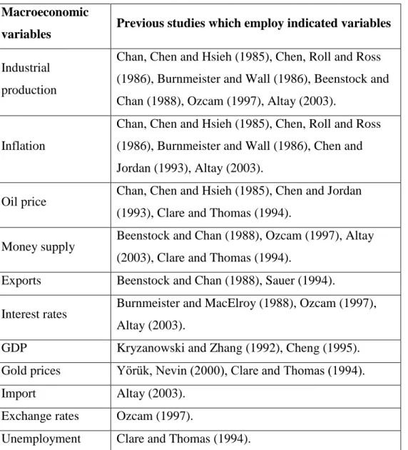
Macroeconomic variables used in previous studies are listed below:

Macroeconomic

variables Previous studies which employ indicated variables

Industrial production

Chan, Chen and Hsieh (1985), Chen, Roll and Ross (1986), Burnmeister and Wall (1986), Beenstock and Chan (1988), Ozcam (1997), Altay (2003).

Inflation

Chan, Chen and Hsieh (1985), Chen, Roll and Ross (1986), Burnmeister and Wall (1986), Chen and Jordan (1993), Altay (2003).

Oil price Chan, Chen and Hsieh (1985), Chen and Jordan (1993), Clare and Thomas (1994).

Money supply Beenstock and Chan (1988), Ozcam (1997), Altay (2003), Clare and Thomas (1994).

Exports Beenstock and Chan (1988), Sauer (1994).

Interest rates Burnmeister and MacElroy (1988), Ozcam (1997), Altay (2003).

GDP Kryzanowski and Zhang (1992), Cheng (1995). Gold prices Yörük, Nevin (2000), Clare and Thomas (1994).

Import Altay (2003).

Exchange rates Ozcam (1997).

Unemployment Clare and Thomas (1994).

Table 1 Macroeconomic Variables and Previous Studies (Source: Türsoy, Gunsel, Rjoub, 2008)

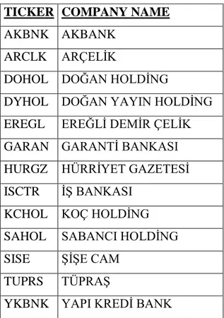
The Stock Returns names and tickers used in the study are listed in Table 2

TICKER COMPANY NAME

AKBNK AKBANK ARCLK ARÇELĠK

DOHOL DOĞAN HOLDĠNG

DYHOL DOĞAN YAYIN HOLDĠNG EREGL EREĞLĠ DEMĠR ÇELĠK GARAN GARANTĠ BANKASI HURGZ HÜRRĠYET GAZETESĠ ISCTR Ġġ BANKASI

KCHOL KOÇ HOLDĠNG

SAHOL SABANCI HOLDĠNG

SISE ġĠġE CAM

TUPRS TÜPRAġ

YKBNK YAPI KREDĠ BANK

Table 2 ISE-National 30 Companies Codes (Source: www.imkb.gov.tr)

Regarding foreign exchange, which is coded as fx, denotes the monthly

percentage change in the real exchange rate index of the currency basket,

based on 1 USD +1.50 EUR, relative price calculations producers for USA

and EURO area and consumer prices for Turkey are used. Exchange rate

policy is an essential anchor for a country regaining its creditworthiness.

Furthermore it has positively contributed to growth of output and exports

and to the expansion of tradable production. To better explain the reasons

for sharp waves, developments in this area should be examined. A floating

“disinflation programme” and its nominal anchor, the crawling – peg system, which had been in effect since the end of 1999, broke down.

In compliance with the floating exchange rate regime, exchange rates were

determined by market conditions. At the beginning of the last global

financial crisis, there was again a new peak on exchange rate graphs.

Exchange rates also affect exports and imports of the country, and the

effects are seen on stock returns.

An economic crisis in South Asian economies took place, which had also

spillover effects on the rest of the world economy. Turkey was not immune

to these effects, especially when the crisis hit the Russian economy, a

significant partner in Turkish foreign trade, in 1998. The crisis precipitated a recession in Turkey’s economy. The year 2000 was a difficult year for exporters, due to the movements in the Euro against the dollar, and a

remarkable increase in oil prices. Further, since 2000 was the first year of

the Economic Program, the exchange rate policy adopted in line with the Program’s inflation target also had negative impact on exports. Following the crisis in 2001, Turkey’s exports rebounded. The underlying reasons

were the deep devaluation that took place due to the introduction of a “floating exchange rate regime” and companies’ strategy of seeking new markets in response to declining domestic demand. Exports continued to

grow strongly in 2002 and 2003. The main reasons behind the strong export

growth in 2003 were the continuous expansion of production, due to weak

domestic demand, the decline in real labor costs, rising productivity,

movements in the Euro / Dollar exchange rate which were favorable to

Turkey. An important are of vulnerability for the Turkish economy during

its 2002 – 2007 growth episode was the rising and gaping current account

deficits. The current Account deficits increased together with growth /

demand and the appreciating currency, rendering the growth unsustainable

after mid-2006.

There was a sharp fall in the value of Turkish exports from October 2008.

The fall in the value of imports was even more pronounced, leading to

slimmer current account deficits from the fourth quarter of 2008. The recent

monthly values indicate that imports started to pick up from March 2009,

while exports continued to stagnate, with the result that the current account

deficit started rising again after March 2009. Another reason for the decline

in Turkish exports was that the share of Turkish exports to its main export

area was counterbalanced by countries like China and India. As far as

foreign trade is concerned, there is a general consensus view that “the recent

global crisis raised costs and constraints in the financial sector in providing

working capital, pre shipment export finance, export credit insurance and

issuance of letters of credit for international trade.

In emerging markets like Turkey, gold is seen as an alternative portfolio

investment tool against bond or stocks. As an investment, gold is typically

viewed as a financial asset that will maintain its value during periods of

political, social or economic distress. As such, gold can provide both

In most cases, it is widely recognized as a hedge against foreign currencies

(such as the US Dollar) and as some measure of inflation. For instance, as

the value of the dollar falls relative to major currencies, the price of gold

tends to move higher, though the correlation is not always perfect.

In the last wave of financial crises throughout the world, gold was

internationally regarded as being money. But unlike cash, it is a far safer

option in times of economic distress. As confidence throughout the world

increases and economies recover, the price of gold is likely to fall back a

little. Another two reasons for the increase in gold prices are the shortage of supply and China’s reserve. As one of the world’s fastest growing economies, China is adding to its gold reserves.

The industrial production index is another macroeconomic variable used in

the study. Industrial production is an indicator of growth in a country.

After the turbulence and volatility of the 1990s and early 2000s, the Turkish

economy recorded relatively high and stable growth rates between 2002 and

mid 2007. However GDP growth started to decline markedly in mid 2007.

The sharpest decline was seen in 2009 as the global financial crisis struck.

The sharp decline in growth is even more strikingly reflected in the monthly

industrial production index. The period analyzed in this study starts with

1999. The 1998 – 1999 recessions, which started with the effects of the

Asian and Russian crises, lasted for 15 months. The 2000 – 2002 recessions,

which followed an exchange rate targeting regime, also lasted for 15 months

August, 2008. As a result, the ip1 exhibits sharp declines during periods of

economic crisis.

M2 is the broadest measure of total money supply. M2 includes everything

in M1 and also savings and other time deposits. M1 is not used in this study;

M1 offers a narrower definition of money supply. The relationship between

money supply and inflation is one of the important elements in

macroeconomic policy, as governments seek to control inflation. Money

supply has a powerful impact on economic activity. An increase in money

supply precipitates increases in spending, since it places more money in the

hands of consumers, making them feel wealthier, driving them to increase

their spending. At the beginning of 2001, the aim of new economic policy in

Turkey was to attain stability by lowering its deficits, bringing down

inflation and achieving higher and more sustainable growth. The IMF

program was at the top of the list.

The preconditions would be created for an “implicit inflation targeting” policy and short – term interest rates were to become critical policy

variables.

For the period 2002 – 2004, in addition to the base money target, net

international reserves become a performance criterion and net domestic

assets an indicative criterion.

In short, all well on the monetary policy side until the end of 2005, the years

2006 and 2007 were both difficult years for monetary exchange rate