Radiation fields of the line source in a cylindrical wire grating

' 0 ^ ■ т д а , '-':к?‘Г-·: ^ V^-'··■'-"·тГ:;’Зі' at# · '/>^*··· T ’■'' ' rS-C'^-'^y-T'h >''-'ÍT't,·^*’,'^ :T^'^·V'r4;7·>·X^!ŞT4:T>.T■^ ;■■ >' ·. vT>?-'^VrrV^ï^..-'K’fî?···. >’"T? t? T'^· ·'·'Wf ■Г'^'*:'6>Л'Г ■ ■ ·ρ**ΓΤ· '^;^. V*/“TV'T "»7^·'·*^^· . .'' ‘ · . '"ГЧ··’" Д'>^·’· T? ’f 'f ^’;->'<>?; '^J3i '^Q'Tí <T-'Ч2 ' ί ^ Σ ι ■.' '" •.," ¿ 7 ‘ѵА ■.'; г.·--' ': ^ ‘. 6 S 3 0

RADIATION FIELDS OF THE LINE SOURCE IN A

CYLINDRICAL WIRE GRATING

A THESIS

SUBM ITTED TO THE DEPARTMENT OF ELECTRICAL AND

ELECTRONICS ENGINEERING

AND THE INSTITUTE OF ENGINEERING AND SCIENCES OF BILKENT UNIVERSITY

IN PARTIAL FULFILLMENT OF THE REQUIREMENTS FOR THE DEGREE OF

MASTER OF SCIENCE

By

Hakan Karapınar

December 1998

Tl¿ 6 5 0 0

• R3

11

I (Xirtify tliat I have read this thesis and that in my opinion it is hilly adeipiate, in scope and in quality, as a thesis for the degrei; of Mastiir of Scienc.e.

Prof. Dr. Ayhan Altinta:^ (Supervisor)

I certify that I have read this thesis and that in my opinion it is fully adiHiiiate, in scope and in quality, as a thesis for the degree of Master of Science;.

Dr.'' V İşaimir Yurchcnko(Co-Supcrvisor)

I certify that I have read this thesis and that in my opinion it is hilly adeciuate, in scope and in quality, as a thesis for the degree of Masteu· of Science!.

I certify that I have read this thesis and that in my eipiniem it is fully aelexjuate, in scope and in quality, as a thesis for the de^gree eif A4aste!r e>f Se:ie!iice!.

Assist. Prof. Dr. Birsen Saka

Approved for the Institute of Engineering and Sedenexis:

Prof. Dr. Mehme^^aray

ABSTRACT

RADIATION FIELDS OF THE LINE SOURCE IN A

CYLINDRICAL WIRE GRATING

Hakan Karapınar

M.S. in Electrical and Electronics Engineering

Supervisors: Prof. Dr. Ayhan Altıntaş

Dr. Vladimir Yurchenko

December 1998

In this thesis, the transmission effect of a grid structure is analyzed. The grid structure is intended to model the metallic support elements of a radome. The total field for the real and complex position line sources surrounded by the grating structure is obtained in both TM and 7'E polarizations in the far-field region.

The grid is considered to be a cylindrical array of perfectly conducting cylinders parallel to the z-axis. The radius of each cylinder is small as com­ pared to the wavelength and the length of the cylinders is infinite.

We started with the study of a single perfectly conducting cylinder illuminated by a line source and obtained the formula for the electric and magnetic fields in the far-field region. Then, we calculated far-zone total field for a set of cylinders which form the surface of the radome as a cylindrical periodic grat­ ing. The equation for the total electric field in the far-field region is found by using superposition and applying the boundary conditions at the conducting cylinders to find scattering coefficients.

Complex line sources are considered to simulate directed beam fields used in practice. The power pattern and directivity are computed for different pa­ rameters of the grating and cylinders. A set of figures is presented to show the relationships between the power pattern, directivity and different parameters of the structure.

Keywords: Grating, directivity, complex source

ÖZET

SİLİNDİRİK IZGARA İÇERİSİNDEKİ BİR ÇUBUK

KAYNAĞIN IŞINIMI

Hakan Karapınar

Elektrik ve Elektronik Mühendisliği Bölümü Yüksek Lisans

Tez Yöneticileri: Prof. Dr. Ayhan Altıntaş

Dr. Vladimir Yurchenko

Aralık 1998

Bu tezde, ızgara yapının alan geçirgenliği incelenmi,ştir. Izgara yapı, meta­ lik elementlerle destekli radoınu rnodellemek için tasarlanmıştır. TM and TE polarizasyonlarında, uzak alan bölgesinde ızgara yapı içerisinde bulunan reel ve karmaşık kaynaklar için toplam elektrik alan çözümleri bulunmuştur.

Izgara, г-eksenine paralel iletken silindirlerden oluşan silindirik dizi olarak düşünülmüştür. Her bir silindirin yarıçapı dalga boyuna göre çok küçük olup, silindirlerin boyları sonsuz olarak alınmıştır. Tek bir silindir ile çalışmaya başlanıp bu silindir için toplam elektrik alan formülü elde edildikten sonra, radomun üzerini periodik dizi şeklinde çevreleyen silindirler için toplam elek­ trik alan formülü bulunmuştur. Uzak alan bölgesindeki her bir silindirin ayrı ayrı oluşturdukları toplam elektrik alan denklemleri süperposisyon kullanılarak bulunup, bu denklemlere, sınır koşullan uygulanarak saçılma katsayıları bu­ lunmuştur.

Pratikte, karmaşık kaynaklar kullanılarak enerjinin yönlendirilmesi simule edilmiştir. Enerjinin yönlendirilmesi ve gücü için tüm veriler, ızgara ve onu oluşturan silindirlerin farklı parametreleri için hesaplanmış ve aralarindaki ilişki bir çok grafik ile gösterilmiştir.

Anahtar kelimeler: Izgara, yönlendirme, karmaşık kaynak.

A C K N O W L E D G M E N T S

I would like to express my sincere gratitude to Dr. Ayhan Altıntaş and to Dr. Vladimir Yurchenko for their supervision, guidance, suggestions, encour­ agement through the development of this thesis.

I would like to thank to Dr. Levent Gürel and to Dr. Biisen Saka for theii reading the manuscript and commenting on the thesis.

I would like to thank to my parents, brother and sisters whose understand­ ing made this study possible.

Sincere thanks are also extended to everybody who has helped in the de­ velopment of this thesis.

Contents

1 INTRODUCTION 1

2 ANALYSIS OF RADIATION THROUGH A RADOME

WITH GRATINGS 4

2.1 Electric Line Source (TM Polarization) Parallel to Single Cylinder 5

2.2 Circular Grating with Many Conducting Cylinders ... 8

2.3 Complex Line Source ... 13

2.4 Magnetic Line Source (TE Polarization) ... 15

3 NUMERICAL METHODS FOR CYLINDRICAL FUNC­ TIONS AND LINEAR EQUATIONS 18 3.1 Computation of Bessel and Hankel Functions... 18

3.2 Solution of Linear E q u atio n s... 23

3.2.1 Elimination Method ... 25

3.2.2 Gaussian E lim ination... 25

4 NUMERICAL RESULTS AND DISCUSSION 28 4.1 Normalized Power P a t t e r n ... 28

4.1.1 E Polarization... 29

4.1.2 H Polarization ... 31

11

4.2 D irectivity... 4.2.1 E Polarization... 45

4.2.2 H Polarization ... 46

4.3 Complex Source P o sitio n ... 56

List of Figures

2.1 Geometry of circular periodic conducting cylinders ... 5

2.2 Electric line source near a circular cylinder, (a) Side view, (b) Top view ... 6

2.3 The geometry of the circular grating with conducting cylinders. 8

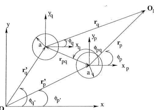
2.4 Geometry of two circular cylinders and their coordinate systems. 10

2.5 Geometry of the complex line source... 13

3.1 \Jn{z)\, Argument: z=60 solid line, z=50T20i dash-dotted line . 20

3.2 |T„(2:)|, Argument: z=60 solid line, z=50-f20i dash-dotted line . 21

3.3 —RelativeError— ... 23

4.1 Power at far zone (for E polarization) for a grating consisting of four cylinders :M=4, kc=62.8, kb=5, beta=0, ka=0.4, N=5. . . 32

4.2 Power at far zone (for E polarization) for a grating consisting of six cylinders :M=6, kc=62.8, kb=5, beta=0, ka=0.4, N=5. . . . 32

4.3 Power at far zone (for E polarization) for a grating consisting of six cylinders :M=6, ka=0.04, kc=3.14, N =4... 33

4.4 Electric field at far zone (for E polarization) for a grating con­ sisting of two cylinders :M=2, kc=62.8, kb=5, beta=0, ka=0.4, N =5... 33

4.5 Power at far zone (for E polarization) for a grating consisting of two cylinders :M=2, ka=0.4, kb=5, kc=62.8, beta=0... 34

IV

4.6 Power at far zone (for E polarization) for a grating consisting of two cylinders :M=2, ka=0.8, kb=5, kc=62.8, beta=0... 34

4.7 Power at far zone (for E polarization) for a grating consisting of fonr cylinders :M=4, ka=0.4, kb=5, kc=62.8, beta=0... 35

4.8 Power at far zone (for E polarization) for a grating consisting of two cylinders :M=2, ka=0.4, kb=5, kc=62.8, beta=(), N=5. . . 36

4.9 Power at far zone (for E polarization) for a grating consisting of four cylinders :M=4, ka=0.4, kb=5, kc=62.8, beta=0, N=5. . . 36

4.10 Power at far zone (for E polarization) for a grating consisting of six cylinders :M=6, ka=0.4, kb=5, kc=62.8, beta=0, N=5. . . . 37

4.11 Power at far zone (for E polarization) for a grating consisting of ten cylinders :M=10, ka=0.4, kb=5, kc=62.8, beta=0, N=5. . . 37

4.12 Power at far zone (for E polarization) for a grating consisting of four cylinders :M=4, kb=5,ka=0.4, beta=0, N =5... 38

4.13 Power at far zone (for E polarization) for a grating consisting of four cylinders :M—4, kb=5, kc=62.8, beta=0, N =6... 39

4.14 Power at far zone (for E polarization) for a grating consisting of four cylinders :M=4, kb=5, kc—62.8, beta=0, N—6... 39

4.15 Power at far zone (for E polarization) for a grating consisting of four cylinders ; ka=0.4, kc=62.8, beta=0, N=5 ... 40

4.16 Power at far zone (for E polarization) for a grating consisting of four cylinders :M=4, ka=0.4, kb=5, kc=62.8, N=5... 40

4.17 Magnetic Field (for H polarization) for free space and for two cylinders :ka=0.4, kb=5, kc=62.8, beta=0, N =5... 41

4.18 Power at far zone (for H polarization) for a grating consisting of two cylinders :M=2, ka=0.4, kb=5, kc=62.8, b eta= 0... 42

4.19 Power at far zone (for H polarization) for a grating consisting of four cylinders :M=4, ka=0.4, kb=5, kc=62.8, beta=0... 42

4.20 Power at far zone (for H polarization) for a grating consisting of six cylinders :M=6, ka=0.4, kb=5, kc=62.8, bcta=0, N=4. . . . 43

4.21 Power at far zoiie(for H polarization) for a grating consisting of four cylinders ;M=4, kb=5, kc=62.8, beta=0, N =5... 43 4.22 Directivity versus Beam Direction (for E polarization) for a grat­

ing consisting of single cylinder:kc=62.8, kb=5; ka=0.4, N=5. . 47

4.23 Directivity versus Beam Direction (for E polarization) for a grat­ ing consisting of two cylinders:M=2, kc=62.8, kb=5;ka=0.4, N=5. 47

4.24 Directivity versus Beam Direction (for E polarization) for a grat­ ing consisting of three cylinders:M=3, kc=62.8, kb=5, ka=0.4, N =5... 48

4.25 Directivity versus Beam Direction (for E polarization) for a grat­ ing consisting of four cylinders:M=4, kc=62.8, kb=5, ka=0.4, N=5... 48

4.26 Directivity versus Beam Direction (for E polarization) for a grat­ ing consisting of five cylinders:M=5, kc=62.8, kb=5; ka=0.2, N=4. 49

4.27 Directivity versus Beam Direction (for E polarization) for a grat­ ing consisting of six cylinders:M=6, kc=62.8, kb=5, N =6... 49

4.28 Directivity versus radius of cylinders (for E polarization) :kc=62.8, kb=5, beta=0, N=5... 50

4.29 Directivity versus grating radius (c) (for E polarization) for a grating consisting of two cylinders: M=2, ka=0.4, kb==5, beta=0, N =4... 50

4.30 Directivity versus frequency (for E polarization) for a grating consisting of two cylinders :M=2, c=1.5m, a=lcrn, b=12cm, beta=0, N =5... 51

4.31 Directivity versus frequency (for E polarization) for a grating consisting of four cylinders :M=4, c=1.5m, a=lcm , b=12crn, beta==0, N=5... 51

4.32 Directivity versus frequency (for E polarization) for a grating consisting of two cylinders :M=2, c=1.5m, a=lcm , b=12cm, beta=0, N=5... 52

VI

4.33 Directivity versus wave length (for E polarization) for a grating consisting of two cylinders :M=2, c=1.5rn, a=lcrn, b=12cm, beta=0, N =5... 52

4.34 Directivity versus Beam Direction (for H polarization) for a grat­ ing consisting of a single cylinder: kc=62.8, kb=5, ka=0.4, N=5. 53

4.35 Directivity versus Beam Direction (for H polarization) for a grat­ ing consisting of two cylinders:M=2, kc=62.8, kb=5, ka=0.4, N=5. 53

4.36 Directivity versus Beam Direction (for H polarization) for a grat­ ing consisting of four cylinders:M=4, kc=62.8, kb=5, ka=0.4, N - 5 ... 54

4.37 Directivity versus Beam Direction (for H polarization) for a grat­ ing consisting of six cylinders:M=6, kc=62.8, kb=5, ka=0.4, N=5. 54

4.38 Directivity versus radorne radius (for H polarization) for a grat­ ing consisting of two cylinders:M=2, kb=5, ka=0.4, N =5... 55

4.39 Position of the complex line source... 56

4.40 Power versus Angle (E polarization) for a grating consisting of four cylinders: kc=62.8, kb=5; ka=0.4, Beta=180 deg, N=5, r0=21ambda and r0=0... 58

4.41 Power versus Angle for a grating consisting of four cylinders: kc=62.8, kb=5; ka=0.4, N=5, r0=21ambda... 58

4.42 Total power versus rO (E polarization)for a grating consisting of a single cylinders:M=l, kc=62.8, kb=5;ka=0.4, Beta=0 deg, N=5. 59

4.43 Total power versus source position (for E polarization) for a grat­ ing consisting of two cylinders:M=2, kc=62.8, kb=5; ka=0.4, N=5, r0=21ambda ... 59

4.44 Directivity versus source position (for E polarization) for a grating consisting of a single cylinders: kc=62.8, kb=5;ka—0.4,

Beta=0 deg, N = 5 ... 60

4.45 Directivity versus source position (for E polarization) for a grat­ ing consisting of two cylinders: M=2, kc=62.8, kb=5; ka=0.4,

Vll

4.46 Directivity versus source position (for II polarization) for a grat­ ing consisting of one and two cylinders: kc=62.8, kb=5;ka=0.4, Beta=0 deg, N—5. ... 61 4.47 Directivity versus source position (for E and H polarizations)

for a grating consisting of two cylinders:M=2, kc=62.8, kb=5; ka=0.4, N=5, r0=21ainbda... 61

Chapter 1

INTRODUCTION

The problem of scattering from a cylindrical surface has aroused the interest of physicists and engineers for many years because of its large domain of ap­ plication in optics, acoustics, radiowave propagation and radar techniques [1]. Also, the penetration of electromagnetic waves through a layered system is always an interesting subject of study which finds many applications [2], for instance in evaluating the performance of antennas surrounded by radorne. Typically, large radar antennas are covered with radoine in order to protect them from weather conditions (rain, wind, sun, etc.) and to enable them to operate continuously without loss of precision.

The design of radomes for antennas may be divided into two separate and relatively distinct classes depending upon whether the antenna is for airborne or ground-based (or ship-based) applications [3]. The airborne radome is char­ acterized by smaller size than ground-based radomes since the antennas that can be carried in an aircraft are generally smaller. The airborne radome must be strong enough to form a part of the aircraft structure and usually must be designed to conform to the aerodynamic shape of the aircraft, missile, or space vehicle in which it is to operate.

A properly designed radome should distort the antenna pattern as little as possible. The presence of a radome can affect the gain, beamwidth, sidelobe level, and the direction of the boresight (pointing direction), as well as change tlie VSWR and the antenna noise temperature. Sometimes in tracking radars, the rate of the change of the boresight can be important. In this study, we have analyzed how directivity and power pattern of antenna are effected by

the grating structure. Here, the source is surrounded by the grating structure. Tlie grating structure is intended to model the metallic support elements of a radome.

In practice, a precise analysis of radome performance is difficult and nearly impossible since the general shape of the radome la,3'cr does not fit into the

frame suitable for exact analysis. One must therefore resort to some ai)prox- imate methods. The basic principle of approximation is to find a canonical configuration to approximate the surface of the dielectric layer. A method of modal cylindrical wave spectrum, which is an extension of the plane wave spectrum surface integration technique [4], is applied to the analysis of a two- dimensional elliptic radome. Previously, far-field solutions for complex line source surrounded by a cylindrical dielectric radome are calculated in [2]. The transmission effect of two-dimensional circular radome with periodic gratings is analyzed in [5]. In this thesis, we have obtained far field solutions for real and complex line sources surrounded by a two-dimensional circular radome with periodic conducting cylinders. In this study, we have assumed that, the transmission effect of the dielectric shell is optimized. Thus, we have neglected this effect.

The aim of this thesis is to analyze the effect of the radoine formed by a grid of perfectly conducting cylinders on the propagation of the electromagnetic waves, and to obtain how directivity and power change with different radome parameters.

The analysis of the scattering from multiple conducting, dielectric or combi­ nation of dielectric and conducting cylinders for incident plane wave is treated by many investigators [6], [7], [8]. However, a rigorous solution to the scatter­ ing from conducting cylinders which are placed on the surface of the grating geometry is not available in the literature for real and complex line sources. Here, the solutions for real and complex line sources which are enclosed by grating with conducting cylinders are derived.

The problem of electromagnetic wave scattering from objects arc treated using different methods. Among those methods are the integral equation for­ mulation [9], [10], partial differential equation formulation and hybrid tech­ niques which combine the partial differential equation method with a surface integral equation or with an eigenfunction expansion [9]. The integral equa­ tion method requires numerical integrations which lead to a system of matrix equations. The order of this matrix equation increases with the electrical di­ mension and complexity of the scattering objects. This technique requires

significant computation time for composite scatterers. On the other hand, to enforce the radiation condition using a partial differential equation method, an approximate absorbing boundary may be used in order to avoid extending the descretized region to infinity. Furthermore, the use of numerical differentiation limits the accuracy of such methods. The hybrid techniques eliminate most of these disadvantages, however, it usually requires more effort in the analytical and numerical implementations [11]. In this thesis, the analysis begins by rep­ resenting the scattered field of each cylinder as a series expansion in terms of cylindrical functions with unknown coefficients. Then, by applying the bound­ ary conditions on the surface of each cylinder and using superposition to obtain a set of linear equations for unknown scattering coefficients which can be writ­ ten in a matrix form. The Gaussian elimination with backward substitution method is used to solve these linear equations.

The outline of thesis is as follows. In Chapter 2 we introduce the basic concept of the techniques and the formulation of the problem. In Chapter 3 we introduce the numerical techniques for generating Bessel functions and for solving a set of linear equations. Numerical results are presented in Chapter 4. Main conclusions follow in Chapter 5.

Throughout the analysis, a sinusoidal-varying time dependence is as suined and suppressed.

Chapter 2

ANALYSIS OF RADIATION

THROUGH A RADOME

WITH GRATINGS

In this chapter, we obtain the general formulas for radiated electric field due to an electric line source and the total radiated magnetic field due to a magnetic line source inside the multicylindrical structure as it seen in Figure 2.1. The cylinders are assumed to be periodically located over a circle of radius c centered around the source. The radius of each cylinder is a.

Both real and complex line sources are considered. Complex line source is used to simulate a directed beam. The wave field is represented as expansion series of cylindrical waves to evaluate the radiation fields. Then, the efi'ect of transmission through the number of perfectly conducting circular cylinders is found. The surface of many practical scatterers can often be approximated by cylindrical structures [12]. We will consider cylindrical waves for both the real and complex-position line sources surrounded by a set of circular conducting cylinders of infinite length.

Obscrvalion Angle

Figure 2.1: Geometry of circular periodic conducting cylinders

Formulation of the problem is initially carried out for a single cylinder with real position electric line source and then extended to the case of rnulticylindiri- cal structure with real and complex position electric line sources.

2.1

Electric Line Source (TM Polarization)

Parallel to Single Cylinder

A line current of infinite length directed along the z axis is assumed to be placed at r' in the vicinity of a circular conducting cylinder as shown in Figure 2.2. The line source is outside the cylinder (r' > a).

The cylinder is also assumed to be infinite in length and its axis is parallel to the line source. If the line source of Figure 2.2 is a tirne-harrnonic electric current of constant amplitude A, the electric field generated everywhere by the source in the free space is found in the following manner.

(a) _(b)

Figure 2.2: Electric line source near a circular cylinder, (a) Side view, (b) Top view

The free space Green’s function G of the line source can be written as

G{r,(j);r',(j)') = I

r-P

|).

(

.

)

This is the well-known two-dimensional Green’s function for the cylindrical wave [12]. From (2.1), the incident field can be found as

k lL

= “ I ’" ’''I) (2.2)

where k^ = 27t/A is the free space wave number and A is the wavelength.

By the use of the addition theorem for Ilardcel functions, we can write (2.2) as k'^T j^inc ^0^6 ^ 4we Uh„r)Hi^Hk„r')ei''^*-*'> r < r' E S .-« , r > r' (2.3)

In the presence of the cylinder, the total field is composed of two parts: the incident field and the scattered field. The scattered field is produced by the current induced on the surface of the cylinder that acts as a radiator.

The scattered field also has only z component and it can be expressed as

l· T °°

„i-co

The unknown coefficients Cn can be found by applying the boundary condi­ tions of

— a, 0 < (p < 27t, z) = 0 ,

to the total field on the surface of cylinder

E to l ^ ^ m c ^ ^ i c a i ^ q

that yields the equation

(2.5)

(2.6)

¡l2 r oo

E [Jn{koa)H^^\kov') -b = 0.

71= -OO

From here, C,i can be found as

1171 (^koG.)

which then yields

(2.7)

(2.8)

E

4we

ES.-»ifW (*^,r')[7„(to>·) - r < r'

For far-field observations (kor > > 1 ) the total electric field of (2.9) can be reduced by replacing the Hankel function Hj^^koi') by its asymptotic expres­ sion

The total electric field in the far-zone can be expressed as

(2.10)

//A [koa)

(2.11)

which can be used to compute more conveniently far-field patterns of an electric line source located near a circular conducting cylinder.

2.2

Circular G rating w ith M any C onducting

Cylinders

In this section, we obtain the general formula for the total electric field at the far zone of a multicylindrical structure. In this geometry which is shown in Figure 2.3, the line source is surrounded by the a grating which consists of many perfectly conducting cylinders.

o

Here, c is the radius of the grating, a is the radius of the each cylinder, Ti and (j)i are the distance and the angle between zth cylinder and observation point for i = 1...M, respectively, with M is the total number of cylinders.

For the structure of four cylinders shown in the Figure 2.3, the total field consists of an incident field coining from the source, and of four scattered fields coming from four scatterers:

j^ lo t __ jjjinc _j_ j^ scat j^ sca t jjjscai _j_ j^ scat

z z z \ z Z z3 zA

(

.

)

The general formula for the total electric field at the observation point for a set of M conducting cylinders on the surface of the radome is [8]

M j g t o l ^ j^ in c scat z m (2.13) rn = l where

E

is the corresponding scattered electric field cornjionent related to r/?,th cylinder and C,nn is the unknown coefficient related to the ?7ith cylinder which includes the effect of all interactions between the cylinders. In the above equations, J„ (i) a n d / / « ( x ) are the Bessel and Hankel functions of order n and argu­ ment .7;.

On the surface of the ith cylinder, the boundary conditions are

M

E T -I- E = 0 at ri = a, 0 < < 27t

m = i

(2,15)

where o is the radius of each cylinder and M is the total number of cylinders. The first terra on the left-hand side of (2.15) represents the incident field at the 7th cylinder, in terms of the local coordinates of this cylinder {ri,(/)i). The second term on the left-hand side represents the scattered electric field from all M cylinders in terms of the local coordinates of each individual cylinder {'I'mAm)· In order to solve for the unknown expansion coefficients Cmn if is then required to express the scattered field from one cylinder in terms of the local coordinates of another cylinder.

10

O,

Figure 2.4; Geometry of two circular cylinders and their coordinate systems.

Using the addition theorem for Hankel functions, one can write the trans­ formation from the (?th coordinate to the pth coordinate as

OO

where > Vp and

fp, = \/r;2 + r;2 - 2r;r;cos((^|, - (/>;)

'I’p,

=

I

(2.17)

(2.18)

' PQ

In the circular grating geometry, = r'p = c and (j/p = where

p = 0,1,..., M — 1 is the cylinder numbers. The transformation from the pth to the ^th coordinates is identical to (2.16) except that the p and q should be interchanged. In order to satisfy the boundary conditions as in (2.5), the total electric field component at the mth cylinder is obtained in terms of the local coordinates of the mth cylinder by using the addition theorem in (2.16):

M scat where E ^ = E ‘Z + E i T + E E S jl2 r 00

E Z = - ^ L

(

.

)

11 1 .2 T oo E ’Z ‘ = - ^ E (2.21) M M oo oo

E

E E E

= “ £■> + ’■(' - 2i;„r;cos(<A;., - and

'■ 7 7n i ·'

If we apply boundary condition for the JTith cylinder

M

E i l = E 'Z + E ’Z ‘ +

E E;r = o

with ?',7i — a , = c and r( = c and use the orthogonal property of the

exponential function we obtain linear equations relating the coefficients

C,

+ E E anJ,(^oa)//i?.U^or™)e-^(’-’'·)^’·

for m = 1 ,...,M and g = —o o ,..., —1 ,0 ,1 ,...,oo. Where (¡)rns is the angle between line source and rnth cylinder, r„i, is the distance between mth cylinder and line source, r,„j is the distance between ¿th cylinder and mth cylinder, and (¡)mi is the angle between zth cylinder and mth cylinder.

The set of equations (2.24) can be written as follows:

M oo

a? = Y :

E

/1 = 1 71= -o o

where 6ih is the Kronecker’s delta function 1 i = h

(2.25)

Sih

0 i ^ h

(2.26)

and the elements h™\ d·" are given, respectively, by

12

d”· = /ig)(*:oo). (2.28)

The elements of A are given by

(2.29)

and the vector C represents the unknown expansion coefficients of the scat­ tered field from the M cylinders.

The set of linear equation can be written in the following matrix form

or more explicitly A = SC, (2..30)

Ai"

AT

smn

c r

where the vectors A and C are of dimension {2N -I- 1)M, N is the truncation number which has to be chosen so that (2.31) has a convergent solution. The

submatrices are nmn . ^ih — ^ f umn U/J Ujjin i ^ h (mutual interaction) i = h (self-interaction) (2.32)

where n, rn = —N , ..., —1,0,1, The inversion of the matrix S yields the solution for the matrix C.

13

2.3

C om plex Line Source

Complex Source Pulsed Beams (CSPBs) are exact solutions of the wave equa­ tion that can be modeled by a time-dependent source located at a complex coordinate point with a proper choice of parameters. Those wave fields are confined in bearn-like fashion in transverse planes perpendicular to the prop­ agation axis while confinement along the axis is due to temporal windowing. Because they have these properties, CSPBs are useful wave objects for gener­ ating and synthesizing highly focused transient fields and for local probing of a medium. Furthermore, as has been shown recently, CSPBs form a new set of basis functions for an exact angular spectrum expansion of source fields [13].

In this thesis, the complex source of time-harmonic line current is consid­ ered. The direction, collimation and directivity of the source field is determined essentially by the imaginary displacement of the source coordinate.

Unlike the real line source, the antenna feeders are not uniform in practice. So, to simulate nonuniform radiators the complex line source is used [2]. In Figure 2.5, a complex line source generating a beam is shown.

Main Beam

14

The line source is placed at a complex location fg which is given by = ■'"4 + — ax + ib{cosPx + sinPy), (2.33) where the parameter 0 gives the direction of the beam and h is related to the beam width. For b=0, the source position is real and radiation is a.xially uniform. Assuming that the source is located at (r,, (/>,,), the field intensity at the observation point (r, 0) can be written as

E ‘r = C I l f \ k , n ) = C (2.34)

for knR > > 1 where

B. — \Jr'^ + J's — 2rrgCos{<l> — (j)s), (2.35) is the distance of the observation point from the source, r,, fo and b are the complex source position, real source position and beam i)arameter vectors given in polar coordinates as = (»"o, </’o), = {'>'$, (ps) and b = (6,0). All angles are measured from the x-axis. The values of Vg and (pg are

Vg = \ / r l - 10 + 2jrobcos0, (2.36) (2.37)

, ro+ jbcos0

(pg = cos (--- ).

In the far field, B. — r - rgCos{<p - (pg) applies in the phase term, B, - r in the amplitude term. Substituting B, into (2.34), the following expression is obtained.

f;!”" =

C-Jko{r-rQCOs{<f>-(f)o))

^kobcos{(f>-P) _(2.38)

which yields a maximum (p = 0 and a minimum at (/> = /? + tt.

The incident field can also be written as a series in terms of the addition theorem:

E f% r) = C £ r >v g . (2.39)

When b = 0, fg = To, the complex line source behaves as a real line source. So, the diflerence between the formulation of total electric field for real line source and complex line source is only in the incident electric field. The for­ mulations for the scattered fields are the same. Thus, the general formula of total field for M number of cylinders in far field region,

oo M

E^0^(rJ) = K £

+ Z

m = l

where M is the total number of cylinders. (p,n is the angle between observation

I ! 27 ‘k

15

2.4

M agnetic Line Source (TE Polarization)

Magnetic sources, although not physically realizable, are often used as equiv­ alent source to analyze aperture antennas. If the line source of Figure 2.2 is a magnetic source and it is allowed to recede to the surface of a cylinder (r' = a), the total field of the line source in the presence of the cylinder would be repre­ sentative of a very thin infinite axial slot on the cylinder. If the line source of Figure 2.2 is a magnetic source with current of 1^, the fields that it radiates in the absence of the cylinder can be obtained from those of an electric line source by the use of duality. Doing this we can write the incident magnetic field by referring to as

H r = - ^ ^ H ^ " \ k o \ r - r ' I).

This can also be expressed as

„ in c ^ I r <

and the scattered magnetic field can be written as

1.2 T

oo

7C“ ‘ = - ^ y - a < r .

(2.41)

(2.42)

(2.43)

where Dn is used to represent the coefficients of the scattered field. Thus, the total magnetic field

Hlot ^ J^inc scat

(2.44)

The corresponding electric field components can be found using Maxwell’s equations

1

jjjiot ___

jwe dr (2.45)

16

In order to find unknown coefficients D„, we apply the boundary condition of

= a , 0 < (/; < 27t, z) — 0 .

From there, can be found as

A, =

Iir 'ih a )

Thus, the total magnetic field in the far field region can be written as

k l l m ^ r ^ J ~ - j k o

(2.47)

(2.48)

Awn V nkoT_yJkor ^ j-[J„(A:or')

Jn%a)

Ilj,^Hkor’) y (2.49)

For multicylindrical structure as it seen in Figure 2.1, the total magnetic field M H t o l ^ f j i n c ^ scat z m m ~ l where jl2 r 00 n = - o o (2.50) (2.51)

is the corresponding scattered magnetic field component related to ?nth cylin­ der and Djnn is the unknown coefficient related to the mth cylinder which includes the effect of all interactions between the cylinders.

The total magnetic field for the mth cylinder is obtained in terms of the local coordinates of the mth cylinder by using the addition theorem in (2.16)

where M

/i“ = //■“ + / / r + E

K

17 M M oo oo

^

E E E

DinUkorjHiXikor^i)

A;

where F r,ni = \J r 'J -I- rP - 2r(,,r^ cos(0(„ - (^') and

The corresponding electric field components can be found using Maxwell’s equations

p i o t ^ 1 d H j t

jwc d r^ (2.56)

If we apply boundary condition for mth cylinder,

M

rM o t __ jznnc I T T iS Ctti I \ rpsco l __ n

^<j>m - ^<t,m + ^<j,rn + L · ^

1=1,17^771

(2.67)

with r,n = o , = c and r[ = c and use the orthogonal property of the exponential function eh’·'^· we obtain line<ar equations relating the coeilicients

Frnq · -j;(A:oa)/7f)(A;or„,,)e-·«^ = M M oo

+ E E A77./;(A:oa)/fil(A:or„„)e-^(''-")^"

form = 1,..., M and q = - o o , ..., — 1,0,1,..., oo. here is the angle between line source and mth cylinder,r,7is is the distance between ?nth cylinder and line

source, rjni is the distance between ith cylinder and mth cylinder, and is the angle between zth cylinder and ?r?,th cylinder. The total magnetic field in the far-field region is computed by using

OO M

771=1

where M is the total number of cylinders, (f>m is the angle between observation direction and mth cylinder and finally, K — ·

Chapter 3

NUMERICAL METHODS FOR

CYLINDRICAL FUNCTIONS

AND LINEAR EQUATIONS

3.1

C om putation o f B essel and Hankel Func­

tions

In this chapter, the numerical computation of Bessel and Hankel functions of the first and the second kind for integer orders and complex arguments are considered. The numerical computation of linear ecpiation {Ax — b) is solved by using Gaussian elimination with backward substitution. The algorithm for Bessel functions makes use of backward recurrence for the computation of Bessel functions of the first kind where applicable, and of Hankel’s asymptotic expansion for large arguments.

Bessel functions of integer order are the natural and general solutions of many radiation, scattering and guided wave problems which are formulated in the cylindrical coordinate system. Bessel functions are also used in the mathe­ matical description of numerous physical phenomena besides electromagnetism. Consequently, their accurate computation is of general importance.

19

Jn{z) and Yn{z), Bessel function of the first and second kind respectively are solutions to Bessel’s differential equation

z^y" + zy' + — n^)y = 0 (3.1)

In this thesis, we generate Bessel functions using the subroutine developed by Anil Bircan [2] following the algorithm presented by Du Toit [14]. In this method, forward and backward iterations are used to compute J,i(z) and Vniz) based on the recurrence relation

2n

Bn+i{z) = — Bn{z) - Bn-\{z) (3.2)

for all orders for a given argument z. From this relation, if Bn{z) and B„_i(z) are known B,i+i{z) is found with increasing N (forward recurrence), if Bn{z) and Bn.{.]{z) is known, jB„_i(z) are calculated with decreasing N (backward recurrence).

Before using this relation, the stability of recurrence should be guaranteed. Any round-off error will be amplified by the factor 2n/z, and accumulation of these errors occur with the repetitive use of (3.2). The relative error are, however, decreasing when the functions are increasing in the process of iteration. So, progressing through increasing value of |B„(z)j appears to be the best strategy.

Therefore, for ./,1(2:) functions, the backward recurrence is stable since

|J,i(z)| are increasing rapidly with decreasing n. For Yn{z)^ when z is complex, the backward recurrence is stable for small n but the forward recurrence is needed for n > r where r is the index corresponding to the minimum of |K„(z)|.

From the Figures (3.1) and (3.2), when z is real or when \Re{z)\ » |/m (z)|, general magnitude of Jn{z) and Yn{z) for a given argument z is approx­ imately constant for n < |z|, but for n > jzj, Yn{z) increases with increasing n and Jn(^) increases with decreasing n. So, all higher orders of Yn{z) can be computed from Yo{z) and Yi{z) by using forward recurrence. All lower orders of Jn{z) can be computed from Jg.^.i{z), Jq{z) which are arbitrary initialized by using backward recurrence.

When z is complex, the same rule still applies for Jn{^) since it decreases with increasing n for all values of n. K (z) can be calculated from Yr{z), Yr+i{z) using forward recurrence for n > r and backward recurrence for n < r where r is the value of n to yield a minimum to F„(z) for a given argument z.

20

log10IJn(z)l

Figure 3.1: \Jn{z)\, Argument: z=60 solid line, z=50+20i dash-dotted line

The algorithm of Jn{z) is started with estimating of the starting point for backward recurrence. The minimum value for q (the starting point for backward recurrence) is found in [2] as

Qrnin

1^1 -b 10.26l.z|‘’"'’'‘i'’i''^ -b 1.8, 1^1 < 25

|z| -b 6.6362|^|°-3'1248i ^ q4^ |^| > 2 5. (3.3)

After finding qmin the normalized constant S is comi)uted. Since Jn{z) is obtained by normalization of Bn{z) Jn{z) - Bnjz) S (3.4) S is computed in [2] as 7 / 2 S = Bo{z) + 2Y^B2k{z) k=l (3.5)

when Im{z) < 1 and

9 / 2

S = BQ{z) + 2 Y ^ { - \ f B 2 k { z ) k=l

21

log10IYn(z)l

Figure 3.2: |F„(z)|, Argument: z=60 solid line, z=50-l-20i dash-dotted line

when Im[z] > 1. After computing S, Jn{z) is calculated by using (3.4).

The algorithm of computing Y,i{z) is started by using Neumann’s expansion = h (in (z /2 ) + r ) M z ) - 2 £ ( - 1 ) ‘ : % ^ 1 , (3.7)

^ k=0 ^

n( z ) = -[(¡n(z/2) + r - 1) J.(^) - (3.8)

7T 2 K [ K i - .IJ

for calculating Yo(z) and Yi{z) using forward recurrence when z is real or when N < \z\ if z is complex. But, when ^ is complex and N > \z\, Yn{z) can be calculated from Yr{z:) and Yr+i{z) using backward recurrence. In [2], r is calculated as r = [|^| + |/m (2:)|/2] (this can be verified in Figure 3.2).

Yr{z) and Yr+i{z) can be determined from Yo{z), Y\[z) and the Jn{z) functions for N < \z\ by using the expansion of the recurrence relation (3.2), in [2]

Bo{z) = Pn{r, z)Br{z) + Pu{r, z)B,..i.i {z), Bi{z) = P2i{r,z)Br{z) + P22{r,z)Br+l{z).

(3.9) (3.10)

22

By using the Wronskian

Jn+i{z)Yn{z) - Jn{z)Yn-\-].{z) =

1\Z (3.11)

and the fact that determinant of the P matrix is unity, d e t(F )= l, Pn{r,z), Pni^iZ), P2i{f',z) and P2 2{r,z) are calculated.

After these, Yr{z) and Yr+i{z) are computed by using

+ ^ 1 ·

Mz^) 7YZ

(3.12)

(3.13)

So, with r, Yr{z) and K+i, Yn{z) is produced by backward recurrence for n < r and by forward recurrence for n > r .

The accuracy of the algorithms was also tested by examining the numerical error in the Wronskian

error = Jn+i{z)Yn{z) Jn{z)Yn+i{z)

-TVZ (3.14)

For illustration, this error is divided by |,7,i.|.i(^)| + |,/„(^)| ,

e = Jn+i{z)Yn{z) - Jn{z)Yn+i{z) -

(2/7T^)|

|‘^n-l-l(^)| + \Jn{z)\ (3.15)

The relative error |c| is representative in all four functions involved.

The result follows when it is assumed that the relative errors in all four functions involved have the same amplitude, but are uncorrelated. This error |el, Jn{z) and Yn{z) for z=120Tl0i are depicted in figure. The relative error is in the order of 10“ ^'’, 10“ ^® which compares favorably with the double precision used in the codes.

23

log10IJn(z)l, log10IYn(z)l, loglOlerrorl “T 10 . _Yn(z) Jn(z) _ _ _ error 0 --10 /v, ^ \ / ( l\l ' 40 --50 L ₅₀ 100 150 order n Figure 3.3: —RelativeError—

3.2

Solution of Linear Equations

A system of n linear equations in n unknown is usually expressed in the general form as follow:

au.-ri + ai2.T2 + = h a>2l^l + fl22-T^2 + ~ f>2

anl^l “h ^n2^2 h — ^n- (3.;i.G)

The coefficients on, ai2, ·.·, Otih are assumed to be floating point numbers as are the right-hand sides &i,&2,---,^n · The problem is to find numbers

x i, X2,...,x,i so that each of the equations in (3.16) is .satisfied. Often it is

convenient to express (3.16) by using matrix-vector notation. That is, we can write

24

where A is the n x n matrix.

Slightly more general and also useful is the uppertriangular form of the system (3.16) in which a^· = 0 if z > j . That is, the coefficient matrix has the form \ ail ^12 · · · o-in 0 022 • ^271 0 n„ (3.18)

In this case, the equations are as follows

Ci22^'2 + ^23^3 + •••^271-^71 = ^2

^ ' 7 1 — . 1 , 7 1 — 1 " h ^ 7 1 — 1 , 7 1 · ' ^ ’ 7 1 ^ ^ 7 7 , - 1

^nn^n — ^^77,· (3.19)

The solution to such a system is easily determined by backsubstituting. That is, the last equation is solved for Xn ,

= K/o.nn, (3-20)

then this value is used in the next to last equation to determine Xn-i ,

Xji-l — (^71—1 0,,i_i^,iX,i)/a,i_i^,i_i, (3-21)

25

3.2.1

E lim ination M eth od

The first method for the solution of equations is just an extension of the familiar method of eliminating one unknown between a pair of simultaneous equations. It is generally called Gaussian elimination and is the basic pattern of a large number of methods that can be classed as direct methods.

3.2.2

G aussian E lim ination

The most frequently used method for solving moderately sized linear systems is also one of the oldest such methods, namely, Gaussian elimination.

The idea of Gaussian elimination is to transform a linea.r system of the general form (3.16) into a system of the special upper triangular form(3.18). The solution is then found directly by backsubstitution. The transformation can be done in such a way that, if exact arithmetic is used, the solution of the triangular system will be the same as the solution to the original system. Of course, computationally the transformation will involve rounding errors. Hence the transformed system will have a solution that may differ somewhat from the solution to the given system. Note, however, that the only error is due to rounding, that is, there is no truncation error in this metliod.

The transformation referred to above is actually a series of transformation in which the coefficients in the lower part of the system are systematically re­ placed by zeros. First of all, note that the following elementary operations on the system (3.16) have no effect on the solution of the system:

(i) An equation can be multiplied by a nonzero constant. That is, each co­ efficient end the right-hand side can be multiplied by the same nonzero number.

(ii) Two equations can be added together and either of the equations re­ placed by the sum.

26

written clown in any order.

To verify that (i) has no effect on the solution is trivial since such an op­ eration really does not change the equation. Also it is clear that (iii) has no effect on the solution. Operation (ii), however, is not quite so simple.

To solve a system of linear equations,

1. Augment the n x n coefficient matrix with the vector of right-hand sides form a n X (n -I-1) matrix.

2. Interchange rows if necessary to make the value of au the largest mag­ nitude of any coefficient in the first column.

3. Create zeros in the second through nth rows in the first column by subtracting an ¡an times the first row from the rth row. Store the an/a u in

1 z = 2,..., n .

4. Repeat steps (2) and (3) for the second through the (n - l)st rows, putting the largest-magnitude coefficient on the diagonal by interchanging rows (considering only rows j to n), and then subtracting o,ij/ajj times the jth row from the zth row so as to create zeros in all positions of the jth column below the diagonal. Store the aij/ajj in aij, i = j -I-1,..., u. At the conclusion of this step, the system is upper-triangular.

5. Solve for Xn from tlie nth equation by

Xn — 0’n ,n - i - l/ ^ ‘7in·

(

.

)

6. Solve for x „ _ i , . T „ _ 2 , from the (n - l)st through the first equation in turn, by

27

X i =

(li: (3.23)

In this thesis, the linear equations of the total electric field for each cylin­ der are obtained by applying boundary conditions on the surface of the each cylinder.

Chapter 4

NUMERICAL RESULTS AND

DISCUSSION

As mentioned in Chapter 1, the aim of this study is to analyze the effect of a circular grating which consists of an array of conducting cylinders on the transmission of electromagnetic fields radiated by a leal oi complex line souice placed inside this structure for both E and H polarization.

In our investigation, we are interested in periodic conducting cylinders. In this chapter, numerical results for two polarizations (L and II polaiizations) aie obtained. For these two cases, the subject is discussed in terms of normalized power pattern and the directivity which represent two important parameters in design problem.

4.1

N orm alized Power P attern

In this section, we have analyzed normalized power pattern. The associated formula for the normalized power i)attern is given as

Pnoitu (4.1)

29

where U''^^ = for E polarization and for H polarization. For far field region the total field is obtained as

= £ .r[./„(A:or,)e·jn{(f)-(t)s) j

M

f Y , (4.2)

in—-\.

where T„„, = Cmn for E polarization and T,nn — D,nn for H polarizal,ion, A4 is the total number of cylinders, (¡),n is the angle between observation direction and mth cylinder, K = — _{' 4iL;e V EKoV'^}J .

4.1.1

Polarization

In order to observe the effect of conducting cylinders on the radiation of the far-held, we have examined power pattern of the source. In the power pattern, normalized power is changed with observation angle (¡). In this chapter, normal­ ized power is plotted as a function of observation angle for different parameters of the structure and sources. The number of cylinders are shown by M and N is the truncation number. We have started to compute power pattern for the case of no interaction between cylinders. Then, we ha.ve included mutual interaction between cylinders. One of the advantages of the projiosed method is the possibility of computing the power pattern of the field scattered by many cylinders including all mutual interactions between the cylinders or without in­ teractions by simply setting all the elements in the off-diagonal submatrices to zero. The interaction component of the scattered field is an important quan­ tity in the multiple scattering. To illustrate the effect of mutual interaction on the total field pattern. Figure (4.1) and Figure (4.2) are plotted. They show the power of four and six identical conducting cylinders each of radius 0.0064A (ka=0.4) which are located symmetrically with respect to x and y-axes and excited by a complex source. The parameters are ka — 0.4, kb = 5 which corresponds to a beam width of 42'’, radome radius (c) of lOA, P — 0 means beam is directed toward cylinder. From these figures, we can say that the scat­ tered field due to the interaction between cylinders must be considered since it causes a discrepancy of 5 to 10 dB especially in the side lobe regions.

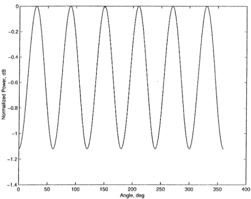
Figure (4.3) shows how the power pattern of the real line source changes with the observation angle {(j)). For a real line source, the directivity of the antenna is unity, because the real line source radiates energy uniformly in all directions. Because of the symmetric geometry, the total field is a periodic function of angle (f> whose period depends on the number of cylinders. The field is scattered more with increasing the number of cylinders. We are interested

30

in complex line source more than in real line source since the former is a directional source and directivity is an important parameter of the antenna.

For a complex line source, the directivity is greater than one {D > 1). The incident field changes with angle <j) as yields a maximum at (p = P and a minimum at = /?-I-tt as it seen in Figure 4.4. This

figure shows the effect of cylinders on radiation of electric field. If the source is in free space (absence of cylinders), amplitude of electric field is maximum at the beam direction and minimum at the opposite direction. If the source is placed between two cylinders, the main beam is distorted and decreased. At the same time, the backscattered field is created by the scatterers.

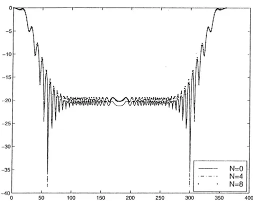
The truncation number {N) shows how many terms in the series (4.2) are needed to obtain convergence. Tlie truncation number required to obtain a specified accuracy depends on the parameters ka and kc. As the radius of the cylinders increases, more terms are needed. However, for very small cylinder radius (a A) which is used in this study, the first nine terms {N = 4) are suIRcient to obtain convergence for kc = 62.8. The Figures 4.5, 4.6 and 4.7 illustrate this result.

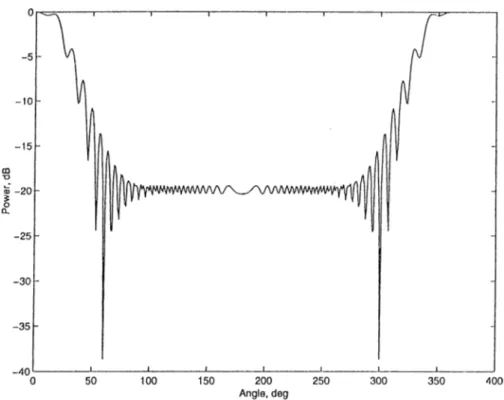
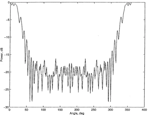
In order to show how power pattern is elfected by the total number of cylinders (M), we have plotted Figures 4.8 through 4.11 for a grating consisting of two, four, six and ten cylinders with ka = 0.4, kb = 5, kc = 62.8, fJ — 0, N — 5 and ?o = 0 (source is in the center of the grating). From these figures, we can see that the main beam is distorted more with increasing the number of cylinders. At the same time, the sidelobes and backlobes of the beam are increased with increasing the number of cylinders as well which is mainly due to the contribution of each cylinder to the scattered field.

The power pattern is dependent on the structure parameters. This de­ pendence is presented in Figures 4.12, 4.13, 4.14 for grating consisting of four cylinders. In these figures, the power pattern is obtained for dilferent radii of grating and cylinders. As observed in these figures, the distortion of the main beam and backscattered field are increased with increasing cylinders ra­ dius and decreasing radome radius. Because, when we decrease radome radius and increase cylinders radius the interactions between source and cylinders increase.

The effects of the beam parameters on the power pattern are observed in Figures 4.15 and 4.16. From these figures, we can say that the sidelobes and backlobes of the beam are decreased with increasing beam width and with

31

choosing beam direction between two cylinders. If we do these, the distortions of the main beam are decreased.

4.1.2

In this section, we liave analyzed magnetic field and power pattern of magnetic line source. The power pattern of magnetic line source ( // polarization) is similar to the power pattern of electric line source {E polarization). Thus, we have not explained figures for H polarization in detail. We have compared E and II polarization in this section.

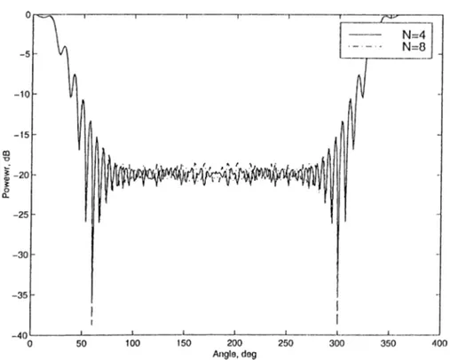
The effect of cylinders on the magnetic field is shown in Figure 4.17. In this figures, the total magnetic field is plotted for two cases. First case, the source is in free space without any cylinder. In this case, the field is maximum when (j) = P (where 0 — Q) and zero when cj) — 0 + n. Second case, the source is in between two cylinders. In this case, the scattered field is created due to conducting cylinders. The cylinders create backscattered field. Figure 4.18, 4.19 and 4.20 present power pattern for different truncation numbers and for different number of cylinders. From these figures, we can see that, the truncation number N equal to four is sufficient to calculate field correctly for ka = 0.4, kb = 5, kc = 62,8 and M = 2,4,6. The total number of cylinders do not affect the main beam, but it affects the backscattered field. If we increase the number of cylinders, the ripple of backscattered field increases mainly due to the number of cylinders at the backward direction of beam increase. The effect of cylinder radius is examined in Figure 4.21. If we increase cylinder radius, the backlobes level increases due to the interactions between source and cylinders.

If we compare the results of E and II polarizations, from the Figures 4.4, 4.5, 4.6, 4.7 and Figures 4.17, 4.18, 4.19, 4.20 we can say that, the effects of the conducting cylinder in E polarization is greater than the effects of cylinders in H polarization. I3ecause, power pattern in II polarization is more sensitive to the size of cylinder than power pattern in E polarization as seen from Figure 4.13 and Figure 4.21.

32

Figure 4.1: Power at far zone (for E polarization) for a grating consisting of four cylinders :M—4, kc=62.8, kb=5, beta=0, ka—0.4, N=5.

Figure 4.2: Power at far zone (for E polarization) for a grating consisting of six cylinders :M=6, kc=62.8, kb=5, beta=0, ka=0.4, N=5.

33

Figure 4.3: Power at far zone (for E polarization) for a grating consisting of six cylinders :M=6, ka=0.04, kc=3.14, N--4.

Figure 4.4: Electric field at far zone (for E

34

Figure 4.5: Power at far zone (for E polarization) lor a grating consisting of two cj'Iinders ;M=2, ka=0.4, kb=5, kc=62.8, beta=0.

Figure 4.6: Power at far zone (for E polarization) for a grating consisting of two cylinders :M=2, ka=0.8, kb=5, kc=62.8, beta=0.

35

Figure 4.7: Power at far zone (for E polarization) for a grating coirsisting of four cylinders :M=4, ka=0.4, kb=5, kc=62.8, beta=0.

3G

Figure 4.8: Power at far zone (for E polarization) for a grating consisting of two cylinders :M=2, ka=0.4, kb=5, kc=62.8, beta=0, N=5.

Figure 4.9: Power at far zone (for E polarization) for a grating consisting of four cylinders :M=4, ka=0.4, kb=5, kc=62.8, beta=0, N=5.

37

Figure 4.10: Power at far zone (for E polarization) for a grating consisting of six cylinders :M=6, ka=0.4, kb=5, kc=62.8, beta=0, N=5.

Figure 4.11: Power at far zone (for E polarization) for a grating consisting of ten cylinders :M=10, ka=0.4, kb=5, kc=62.8, beta=0, N=5.

38 -5 -10 -15 I -2 0 -25 -30 35 --40 \ ; ■ r ' ■ \k ■' ML· . ' . 1/ ■ z ' V ■ .V ' ' - M / x ' I ■' 1/' ' , U \ ’ I • V·* ,:***· A*r r * ' . III i c=4*lam bda — c=5*Iam bda * c=10*Iambda 50 100 150 200 250 Angle, deg 300 350 400

Figure 4.12: Power at far zone (for E polarization) for a grating consisting of four cylinders :M=4, kb=5,ka=0.4, beta=0, N=5.

39

Figure 4.13: Power at far zone (for E polarization) for a grating consisting of four cylinders :M=4, kb=5, kc=62.8, beta=0, N=6.

Figure 4.14: Power at far zone (for E polarization) for a grating consisting of four cylinders :M=4, kb=5, kc-62.8, beta=(), N=6.

40

Figure 4.15: Power at far zone (for E polarization) for a grating consisting of four cylinders : ka=0.4, kc=62.8, beta=0, N=5

Figure 4.16: Power at far zone (for E polarization) for a grating consisting of four cylinders :M=4, ka=0.4, kb=5, kc=62.8, N=5.

41

Figure 4.17; Magnetic Field (for H polarization) for free space and for two cylinders :ka=0.4, kb=5, kc=62.8, beta=0, N=5.

42

Figure 4.18; Power at, far zone (for H polarization) for a grating consi.sting of two cylinders :M=2, ka=0.4, kb=5, kc=62.8, beta=0.

Figure 4.19: Power at far zone (for H polarization) for a grating consisting of four cylinders ;M=4, ka=0.4, kb==5, kc—62.8, beta=0.

43

Figure 4.20: Power at far zone (for H polarization) for a grating consisting of six cylinders :M=6, ka=0.4, kb=5, kc=62.8, beta=^0, N=4.

Figure 4.21: Power at far zoiie(for H polarization) for a grating consisting of four cylinders :M=4, kb=5, kc=62.8, beta=0, N=5.