A Simple Dynamic Applied General Equilibrium Model of
a Small Open Economy: Transitional Dynamics and Trade Policy
Xinshen Diao, Erinc Yeldan and Terry L. Roe**2
A dynamic general equilibrium model of a small open economy is presented to investigate the transition properties of out-of-steady state growth paths in response to trade policy shocks. With the application of the so-called Armingtonian commodity system of static CGE models, we quantify the nature of the transition path and the convergence speed towards the respective steady state under alternative parametrization of the substitution elasticities and of trade policy instruments.
I. Introduction
The applied (computable) general equilibrium (CGE) model has been widely used as a tool for trade reform and tax policy analyses for both developing and the developed countries. Yet, in spite of their Walrasian structure, the traditional (static) CGE models cannot capture intertemporal economic behavior, such as saving and investment decisions, in a theoretically consistent fashion. The treatment of dynamics in the CGE models of the static-genre depends on parametrization of fixed saving rates out of disposable income, and on ad hoc macro closures for the investment demand. The lack of theoretical foundations for such intertemporal decisions and the element of arbitrariness contained therein are clearly not consistent with the behavior of economic agents, who otherwise are regarded as rational optimizers in the solution to their within-period problems. This obvious inconsistency did not escape from the attention of many modelers (see, e.g., Srinivasan (1982), Bell and Srinivasan (1984), Mercenier (1994)). There is now a growing interest in the application of intertemporal dynamic equilibrium theory to real economies with an attempt to incorporate optimal forward-looking behavior of rational agents into the CGE framework. Recent contributions include Wilcoxen (1988), Ho (1989), Jorgenson and Wilcoxen (1990), McKibbin (1993), Mercenier (1993, 1995), Go (1994), Keuschnigg and Kohler (1994, 1995), and Devarajan and Go (1995). This literature attests that, as an intertemporal structure is built into relatively complex multi-sector dynamic GE models, issues such as the nature and causes of transitional (out-of-steady state) dynamics become difficult to evaluate. This often leads to ambiguities concerning the dependence of modeling results and of the transitional path on the model structure itself.
** We are grateful to Jean Mercenier, Agapi Somwaru, Elamin Elbasha, Martin Valdivia, Serdar Sayan, one anonymous Journal reviewer and the participants of the workshops at Bilkent, METU and ERS/USDA for helpful comments and critical suggestions.
** Research associate, University of Minnesota, associate professor, Bilkent University, professor, University of Minnesota, respectively.
The theoretical structure of the transitional dynamics bears importance, as the optimal saving and investment behavior of economic agents in response to policy shocks would depend on the characteristics of the transitional adjustment path. This, in turn, would call for different resource allocation processes, with different transitional rates of growth. It is our purpose in this paper to respond to these issues within the context of a simple two-sector dynamic model, and to document the key role played by the celebrated Armington specification used by most static CGE models, for accommodating transitional (out-of-steady state) dynamics. It is known that a small open economy would not experience transitional dynamics, if (1) international capital markets are perfect, and (2) adjustment costs on investment do not exist. This problem is referred in Barro and Sala-i-Martin (1995) as a “counter-factual” result. The problem is widely discussed for single-sector growth models, and is addressed by specifications which restrict capital flows, and/or permit adjustment costs for investment (Abel and Blanchard (1983)), King and Rebel (1993) further studied, quantitatively, aspects of transitional dynamics in a variety of neoclassical models which sustain intertemporally optimizing agents. They report wide sensitivity for growth paths against parametric changes of various rates governing dynamics.
It is easy to show that in a multi-sector model, the aforementioned counter-factual result still persists. In this paper we attempt to show that, with the introduction of imperfect substitution between the own good (produced and consumed domestically) and foreign good, out-of-steady state dynamics are observed, irrespective of adjustment costs on investment.1 The paper presents the model and model specification in Section II. The dynamic results with and without Armington assumption are discussed in the third section by a two-sector model using 1990 Turkey’s Social Accounting Matrix (SAM) data, and the counter-factual problem is shown to be overcome by accommodation of imperfect substitution. In the fourth section, we study the effects of the substitution elasticity between the own and the foreign good on the transitional paths and on the pace of convergence towards the steady state. Section V focuses on the analysis of the dynamic effects of trade liberalization, with emphasis on changes in investment, trade deficits, and intertemporal consumption smoothing. To illustrate such dynamic adjustment processes in major economic variables, the simple two-sector model is expanded to include more production sectors, base on the same database.
II. A Dynamic Model for a Small Open Economy
For the purpose of this paper, the model specified in this section is much simpler than most of dynamic applied GE models in the literature. By such simplification, we can easily observe some similarity, instead of differentiation, among the current dynamic applied GE modeling literature, i.e., a dynamic applied GE model, with some modification, is an extended neoclassical theory of exogenous growth.
The economy is small in the sense that it faces perfectly elastic supply of and demand for final goods in the world commodity markets, and perfectly elastic supply of and demand
1. This specification is known as the Armington composite system in the traditional CGE literature (See, Armington (1969)).
for capital assets in the world financial capital market. There are two production sectors, agriculture (A) and non-agriculture (N ), employing two primary inputs, labor (L) and capital (K). Labor and capital are mobile between sectors, but not mobile internationally. The aggregate supply of labor is fixed with no population growth envisaged.2 Capital, on the other hand, is accumulated by forgone final outputs from both sectors. To simplify the model, we further ignore technological change.3
1. The Household and Consumption/Savings
The representative household owns labor and all financial wealth, and allocates income to consumption and savings to maximize an intertemporal utility function over an infinite horizon. We assume no independent government consumption and investment. All government tax revenues are transferred to households in a lump sum fashion. For purpose of numerical implementation, the intertemporal problem is formulated in discrete time. The household’s discounted utility of the temporal sequence of aggregated consumption over an infinite time horizon is:
(1)
where is positive and represents the rate of time preference, is instantaneous felicity at each time period, is instantaneous aggregate consumption generated from two final
goods, , :
, (2)
where , and . The household maximizes (1) subject to an intertemporal budget constraint:
(3)
where represents the discount factor from time to time , is instantaneous interest rate at time is the consumer price index such that ; is the wage rate; is the lump sum transfer of government revenues; and is
2. This specification has no real effects on the model, since, alternatively, we could normalize all variables in per capita terms.
3. This implies that the exogenous growth rate associated with productivity change is set to zero. Of course, the transitional growth associated with movement from an initial capital stock toward the steady-state equilibrium remains.
the value of the household’s initial financial wealth.
In an open economy, the representative household’s initial financial wealth, , is not limited to the value of the capital stock, to be denoted . If the value of capital stock exceeds household’s assets, the difference, , then corresponds to net claims by foreigners on the domestic economy. Let be the domestic c ountry’s net debt to foreigners, then the household wealth becomes . The flow of current income generated from financial wealth includes current income from capital stock, minus interest payments on foreign debt. Households allocate their aggregate income flows between consumption and savings. Thus, the current period budget constraint for the household is:
(4)
where is household savings; is the value of aggregate consumption expenditures; is current capital rental price, and is interest payment on the outstanding foreign debt. The Euler equation (derived from first order condition of utility maximization) implies that the marginal utility across two adjacent periods satisfy the following condition:
(5)
where is the derivative of the utility function at time with respect to the aggregate consumption . Equation (5) implies that, the marginal rate of substitution between consumption at time and is equal to the ratio of the consumption price index at
time and .
A sequence of aggregate household consumption and savings are determined simultane-ously from Equation (5). As financial capital is assumed to be perfectly mobile, households view bank deposits and foreign assets as perfect substitutes. Finally, since this is a small open economy, the subjective discount rate is set equal to the world interest rate.
2. Firms and Investment
The major difference of model specifications among the dynamic applied GE literature is the specification for firm and investment. For example, each individual firm can be an investor, such as in McKibbin (1993), or the representative household makes saving/investment decisions, such as in Mercenier (1995). However, under perfect foresight, such different specifications would have a similar allocation of resources. In this paper, in the absence of capital adjustment costs and with constant returns to scale technology and inter-sectoral factor mobility, we assume that producers only maximize temporal profits. Competition among firms ensures that the equilibrium rental price for capital, , is such that it is equal to the value of marginal product of each industry, , and also it equilibrates the demand
for capital with its stock. The value added function for a representative firm in each sector is of Cobb-Douglas, while the intensities of intermediate inputs are fixed.
The aggregate capital stock is managed by an independent investor who decides on investment and passes all profits to the households. This setup is inspired from Willcoxen (1988) and Ho (1989). For a multi-sector model, the introduction of this bank artifact serves to isolate the capital pricing and investment decision from household consumption and saving decisions. The investor chooses a time path of investment to maximize the discounted profit over an infinite horizon:
(6)
subject to capital accumulation constraints:
(7)
where is the value of investment at , is gross addition to physical capital, and is a constant capital depreciation rate. New physical capital, , is a composite good produced from two final goods, i.e., , where is demand for good used to produce new capital at time . We assume that the technology to produce capital equipment exhibits constant returns to scale, hence the unit cost to produce capital equipment is uniquely determined by the price of the two final goods, and that there are no additional capital installation costs beyond the costs of the final goods used in capital good production. Hence, at equilibrium with a positive level of investment, the value of each unit of capital equipment equals its unit cost. Thus, , where is the cost for each unit of . The Hamiltonian of the problem is
(8)
Differentiating with respect to the control variable , the equation equilibrates the shadow price of capital good, , with the production unit cost of capital:
(9)
and differentiating with respect to the state variable we obtain the Euler equation for the investor:
Substituting Equation (9) into (10), we obtain the no-arbitrage condition as follows:
(11)
This Condition indicates that the total returns to capital have to match the return to a perfectly substitutable asset of size . The left side of Equation (11) represents the returns from a perfect substitutable asset of size , and the right side of (11) is the total returns from one unit of capital equipment, which includes: “divide nds” from capital-ownership at each period, minus the loss of the value of capital equipment caused by depreciation, , plus a claim to an instantaneous capital gain (or loss) which is, , if the cost to produce one unit of capital changes over time.
3. Foreign Sector and Foreign Debt
Following the traditional CGE folklore, the model incorporates the Armingtonian composite good system for the determination of imports, and the constant elasticity of transformation (CET) system for exports. In this structure, foreign demand for each good in the domestic economy is derived from a CET function, while the domestic demand for the domestically produced and foreign goods are imperfect substitutes of each other. In each time period, the difference between the value of capital investment, , and the household savings, , is covered by the increase in foreign debt. The increased foreign debt has two components: trade deficit, denoted by , and interest payments on outstanding foreign debt, . If and are both positive, debt is accumulated over time. Thus, foreign debt evolves as follows:
(12)
where a positive implies a trade deficit. 4. Equilibrium
Intertemporal equilibrium requires that at each time period, (i) denote demand plus export demand for the output of each sector equal its supply: (ii) demand for labor equals its supply; and (iii) aggregate investment equals household savings plus net increase in the foreign debt. Under the steady state equilibrium path, the following constraints must also be satisfied:
(14)
(15)
Equation (13) implies that at the steady state, the marginal return of capital normalized by the marginal value of capital is constant and equals to the interest rate plus depreciation rate; hence the marginal cost of investment and the capital rental rate are also constant. Equation (14) implies that investment just covers the depreciated capital; hence the stock of capital per labor remain constant. Equation (15) states that the debt is constant. Furthermore, if the economy experiences debt in the steady state (i.e., is positive), then it has to have a trade surplus to pay interests, i.e., has to be negative. Also, at the steady state, when the country ceases to borrow from foreigners, domestic household savings have to be equal to the value of aggregate investment.
III. Instantaneous Convergence versus Out-of-Steady Dynamics 1. Determination of the Instantaneous Saving Investment Balance
Satisfaction of the aggregate saving-investment balance constitutes the main mechanism for achieving instantaneous macro equilibrium for the economy. Given the intertemporal utility functional of households, consumption and savings are determined endogenously from optimal conditions. For a small open economy, world price for the final good and interest rate faced by the households are exogenous. Thus, in the absence of exogenous shocks, household consumption is constant over time. Furthermore, as the unit cost of capital equipment is uniquely determined by the prices of find good, is also constant. Hence, Equation (11) can be replaced by its steady state condition given in Equation (13), and both the supply of and demand for investment become indeterminate.
For a closed economy, investment is passively determined by aggregate domestic savings. In contrast, for an open economy, investment can also be financed through foreign borrowing, and is not necessarily equal to aggregate domestic savings. since investment demand is independent of the household saving decision, the steady state level of capital stock can be reached through an instantaneous adjustment of foreign borrowing. That is, regardless of the size of the gap between the current (out-of-steady state) level of the capital stock and its steady state level, once the economy is opened up, the capital stock rises (falls) to reach its steady state level immediately through foreign borrowing (lending); i.e., the system admits no transitional dynamics following a shock. For a discrete time model, as specified in this paper, since the previous cost of investment affects current-period investment (see Equation (11)), a new steady state is approached in one period following the shock. This is in contrast of a continuous time model, where the convergence rate from the initial steady state to a new one is infinite (Barro and Sala-i-Martin (1995)).
We use a dynamic numerical example to document this non-transitional path property. Except for imperfect substitutability in foreign trade, the model is based on the algebraic
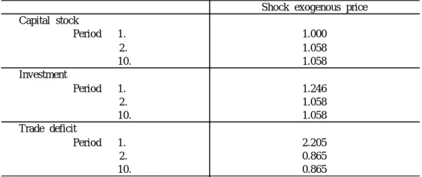
structure of the dynamic applied GE model discussed in the following sections, and is run by using the General Algebraic Modeling System (GAMS).4 Starting from the initial steady state, we shock the economy through a parametric increase of the relative price of agricultural products by 1%. We observe that all endogenous variables converge to their steady state level in the period immediately following the shock. Table 1 presents the results. We omit the values of the related variables in period 3 - 9 and after period 10, since they are exactly same as in period 2 and 10.
Table 1 Numerical Test for Transitional Dynamics Shock exogenous price Capital stock Period 1. 2. 10. 1.000 1.058 1.058 Investment Period 1. 2. 10. 1.246 1.058 1.058 Trade deficit Period 1. 2. 10. 2.205 0.865 0.865
2. Transitional Dynamics under the Armington Commodity System
Now we introduce the traditional Armington and the Constant Elasticity of Transformation (CET) specifications into the model. All the Armingtonian and CET functions are specified in the within-period context, and hence are not affected by the dynamic specification of the model (see Appendix I for the algebraic specification). In each sector, the good produced for the domestic and for the export markets are not perfectly homogeneous. This imperfect substitution is described as one of constant elasticity of transformation (CET) function. Similarly, for consumers and investors, goods imported form abroad or produced domestically are not identical. This imperfect substitution relation is reflected with a constant elasticity of substitution (CES) Armington function. To simplify the analysis, we assume that the composite goods used for consumption are identical to their use in investment.
With the Armington and CET specifications, prices faced by the domestic agents are to be referred as “composite” prices. The price faced by producers is a composite of the price of the good produced for the domestic market and for export, while the price faced by consumers and investors is a composite of the prices of the domestic good and imported good. Export and import prices are world market prices adjusted by trade policy instruments, viz. export tax/subsidy or import tariff. Under this specification, the domestic good price 4. See Brooke, Kendrick and Meeraus (1988).
can no longer be exogenously given, and has to be determined by supply and demand conditions of the domestic market. Hence, supply of input factors, such as labor and capital stock, affect and determine the price levels. The marginal value of capital, which equals the unit cost of investment, becomes a function of the composite price system, which in turn is a function of the aggregate capital stock. That is, through the composite price system, the size of capital stock, and hence the level of investment itself, enter the unit cost function of investment. Thus, the no-arbitrage condition (Equation (11)) can now serve as an implicit investment demand function, and with imperfect substitution in trade, investment demand can be independently determined with the aid of this equation. Hence, a non-steady-state transition path for investment adjustment on the stock of capital can now be observed for a small open economy. IV. Effects of Substitution Elasticities on the Speed of Convergence and Transition Paths With the Armingtonian specification, the transitional path, and hence the speed of convergence, depend upon the elasticities of substitution between goods produced at home and abroad, and the size of the shock. For a given shock, if the own goods can easily be substituted by foreign goods, then the resultant changes in the key dynamic variables, such as investment and debt, along transitional paths are larger, and the new steady state is “approached” in a relatively shorter time. If, per contra, the own good is a poor substitute for foreign goods, then changes in the dynamic variables are smaller, and the transitional dynamics are protracted.
We test the effects of elasticity of substitution and the extent of the shock on the pace of convergence to a steady state with the aid of a two-sector dynamic GE of the Turkish economy. The model is based on an aggregated 1990 Turkey SAM (Kose and Yeldan (1996)). We shock the model implementing full tariff liberalization in both sectors. We choose different elasticity rates for the Armington and the CET functions and observe different transitional paths along with different convergence periods. The results clearly show the influence of the elasticities of substitution on the transitional dynamics, which underscores the importance of careful specification of these parameters when such a model is used for policy analysis.
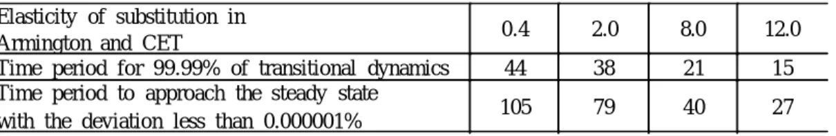
The simulation results portraying the transitional paths of four dynamic variables, investment, stock of capital, trade deficit and foreign assets (negative of the foreign debt), are depicted in Figures 1 - 4, while the terminal periods when the new steady state is approached approximately are documented in Table 2. Two different indicators where selected to represent the time periods needed to converge to a steady state: the first is the time horizon when 99.99% of the transitional life of the main variables is realized; and the second is the time period when all endogenous variables cease to change (by less than 0.000001%). As changes on the endogenous variables become insignificant along their transition paths and convergence to a new steady state is attained, the results are truncated at period 14, a point while 99% of transitional life of each variable is accomplished (Figures 1 - 4). For various elasticities, the paths of transition and the associated convergence periods are diverse. We find that, when tariffs are eliminated, the lower the substitution possibilities between the foreign and the own goods, the smaller are the resulting deviations of the endogenous dynamic
variables along their out-of-steady state paths of transition. Regarding the speed of convergence, on the other hand, the lower the substitution possibilities between the foreign and the own goods, the longer is the time path of convergence to the new steady state (see Table 2).5
Table 2 Effects of Composite Trade Elasticities on the Speed of Convergence Elasticity of substitution in
Armington and CET 0.4 2.0 8.0 12.0
Time period for 99.99% of transitional dynamics 44 38 21 15
Time period to approach the steady state
with the deviation less than 0.000001% 105 79 40 27
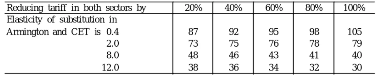
Next, we study the effects of the size of the shock on the paths of transition. We choose different tariff rates together with selected substitution elasticities. We observe that the extent of tariff liberalization affects the transition paths and convergence horizons in consistent way6 (see Figures 5-8 and Table 3). When the elasticity of substitution between the foreign and the own goods in specified at level 0.4, the pace of convergence after eliminating all tariffs is 18 periods slower than that when tariffs are reduced by 20%. When the substitution elasticity is increased, such differences become smaller. Table 3 shows that when the substitution elasticity is increased to 2.0, the difference in the speed of convergence for the same two tariff rate cut scenarios reduces to 6 periods. This is due to the fact that with higher substitution possibilities, the model tends to behave as “a small open economy model with homogeneous goods”. In contrast, when the foreign goods cannot easily be substituted with the domestic good, different tariff rates not only generate different steady state paths, but also different time horizons. In general, the greater the reduction in tariff rates, the longer is the adjustment path to the new steady state. However, this generalization fails when the elasticity of substitution is “very large ”. As we document in Table 3, when elasticities of substitution are on the order of 8.0 or 12.0, the pace of convergence is more rapid after eliminating all tariffs in comparison to partial tariff liberalization.
V. Dynamic Effects of Trade Liberalization
In this section, we study the dynamic effects of tariff-liberalization at greater length. For this purpose, we expand the simply model to include five production sectors, which include agriculture (AG), consumer manufacturing (CMF), producer manufacturing (PMF), materials (INM) and services (SER). We set the trade substitution elasticities at 2.00 and calibrate the initial steady state using the 1990 Turkey SAM (see Appendix II for the calibration strategy).
5. Clearly, the transitional path is also affected by the value of the rate of time preference, . We chose = 0.112 in the experiments. If households discount future at a higher rate, the speed of convergence would be faster. This observation is very much in the spirit of King and Rebelo (1993).
6. It has to be noted that our measure of “the speed of convergence” is a poor benchmark in quantifying and ranking alternative out-of-steady state dynamic paths. Nevertheless, we utilize this measure due to its simplicity in conveying our basic message that, out-of-steady state paths are dependent on alternative parametrization of the substitution elasticities and the policy instruments. For more accuracy on the speed of convergence to the respective steady states, metrics developed in King and Rebelo (1993) can be utilized.
Table 3 Tariff Reform and Convergence to Steady State under Different Elasticities
Reducing tariff in both sectors by 20% 40% 60% 80% 100%
Elasticity of substitution in Armington and CET is 0.4 2.0 8.0 12.0 87 73 48 38 92 75 46 36 95 76 43 34 98 78 41 32 105 79 40 30 After eliminating all existing tariffs in period 1, according to our convergence criteria, a new steady state is approached 100 periods later, 20 periods slower than in the simple model. This implies that given substitution elasticity, the aggregation criteria also affect the convergence horizons.
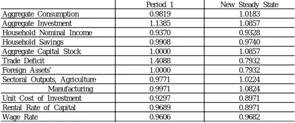
A key difference between the dynamic versus the static modeling of general equilibrium lies in the intertemporal changes in household savings and investment along the transition paths. In a static model, savings and investment decisions are not based on any “forward-looking optimization”. Households are typically assumed to save a “fixed” share of their income, while investment decisions depend on historical shares or current rates of return to capital. In a dynamic GE model, the saving and investment rates are determined as a result of dynamic optimization process based on a sequence of present and future prices, and would change along their transitional path in response to changes in the policy instruments. This, in turn, will have repercussions on all other choice variables of both the consumers and firms. We complement our previous results in Figures 9-12 and Table 4. We depict the transitional paths of the unit cost of the capital investment versus the capital rental price in Figure 9; household aggregate consumption and savings in Figure 10; and finally, selected sectoral exports and imports in Figures 11 and 12, respectively. Table 4 shows changes in the level of the key macro and micro variables upon impact, when the shock is introduced (Period 1), and in the new steady state. All variables are expressed as ratios to their base-run steady state levels.
In general, simulation results indicate that elimination of import tariff would cause a drastic dynamic adjustment in investment, especially at the period of the shock. On the other hand, consumption adjustment is relatively smoother. Wage and capital rental rates fall, which causes a fall in the nominal household income. The level of the intertemporal utility rises by 0.6% compared to the “base-run”.
With an intertemporal utility function and the hypothesis of perfect foresight, the model exhibits permanent income-type of behavior, and current consumption decisions depend on present and future prices and income earnings. Eliminating the tariffs lowers the level of imported goods’ prices and hence the household nominal income. The decline in the household nominal income affects private savings adversely. However, household savings fall less than the decline in the household total income, i.e., saving rate rises. Furthermore, since aggregate consumption expenditures are fixed in nominal terms, changes in the household nominal income following the shock are mainly reflected by adjustments in intertemporal savings (see Table 4 and Figure 10).
Table 4 Dynamic Effects of Tariff Liberalization (Ratios to the Base-Run Steady State Values)
* Trade deficit is observed in the data. See Appendix II for details.
Period 1 New Steady State
Aggregate Consumption 0.9819 1.0183
Aggregate Investment 1.1385 1.0857
Household Nominal Income 0.9370 0.9328
Household Savings 0.9908 0.9740
Aggregate Capital Stock 1.0000 1.0857
Trade Deficit 1.4088 0.7932
Foreign Assets* 1.0000 0.7932
Sectoral Outputs, Agriculture 0.9771 1.0224
Manufacturing 0.9971 1.0824
Unit Cost of Investment 0.9297 0.8971
Rental Rate of Capital 0.9689 0.8971
Wage Rate 0.9606 0.9682
Investment demand displays higher elasticity in response to trade liberalization. Changes in the investment path are determined by changes in returns to capital and the cost of new capital goods, i.e., changes in and . As discussed above, in the absence of adjustment costs on capital installation, the price of a new capital good is always equal to the costs of its production. Since a reduction on tariff rates lowers the Armingtonian composite prices, costs of producing capital goods fall, and investment rise. Simulation results reveal a sudden adjustment in the investment level during the first period when the model is shocked by the exogenous change in trade policy. After this jump, investment converges to its new steady state smoothly.
The transitional path of aggregate investment is further affected by the rental costs of capital. Increased capital stock leads to a decline of its factor remunerations. Compared with base run steady state, the rental price of capital falls by 3% initially, and by 10% in the new steady state (see Table 4). However, the no-arbitrage condition requires that during the transition path, with interest rate held fixed, the decline in investment costs has to precede the decline in the capital rental price. That is, the returns from capital have to rise over time relative to the cost of producing capital equipment; otherwise, the dynamic equilibrium condition of no-arbitrage opportunities would be violated. Figure 9 traces this proposition. As observed, along the transition process, the path of lies above the path of price of capital equipment, , in the early phases of dynamic adjustment, and hence aggregate investment enjoys a further positive inducement (see Equations 10 and 11). Once and are equalized and cease to change, a new steady state is attained.
Simulation results reveal a sudden increase in the trade deficit during the period of the shock. This is mainly caused by the surge in investment. With a relatively “smoother” consumption path, the surge in investment has to be financed through foreign borrowing; and thus, the increased trade deficit reduces foreign asset holdings (see Appendix II). As investment converges
to its steady state smoothly after its initial surge, the trade deficit is on a declining trend and falls further below its base-run level given by the initial data from the sixth period - onwards (Figure 3 for e = 2.0). At the new steady state, the trade deficit and holdings of foreign assets stabilize, where they remain 20% lower than their comparable levels in the base-run.
Data suggest that non-agricultural goods (industry and services) are used more intensively in the production of the investment good. Thus, in response to the rise in investment demand, the aggregate demand for the non-agricultural goods increases faster than that of agricultural goods, and hence the production of non-agricultural sectors. As a generalization, if a country’s per capita investment demand is high, the consequent dynamic effects on non-agricultural trade would be greater than those of the agricultural trade (Figures 11-12).
VI. Concluding Comments
In this paper we developed a multi-sector dynamic general equilibrium model of a small open economy to investigate the properties of out-of-steady state paths in response to trade policy shocks. Using aggregated data from the Turkish economy, we built on the existing stock of literature on the nature of transitional dynamics by highlighting the importance of the so-called Armingtonian commodity system - a typical artifact of most static CGEs. We find that parametric changes on the degree of imperfect substitutability between the own goods and foreign imports/exports affect both the duration and nature of convergence to the respective steady state.
Furthermore, working with a simple trade policy experiment (complete tariff liberali-zation), we investigated the paths of key dynamic variables, such as consumption and saving decisions, capital accumulation and the current account balance. Given the growing interest on bridging the gap between the qualitative imperatives of the theoretical literature on growth economics and the quantitative applications of this body of work on policy directed research, we believe that the modeling effort presented here will serve as a fruitful step towards understanding the underlying nature and interaction between the trade policy, capital accumulation and growth in real-world economies.
Appendix I Equations and Variables in the Model
A.1. List of Equations
The time-discrete intertemporal utility
(A.1)
(A.2)
Within period equations (time subscript is skipped). A.1.1. Armington functions
(A.3)
(A.4)
(A.5)
A.1.2. CET functions
(A.6)
(A.7)
(A.8)
A.1.3. Value added
(A.10)
A.1.4. Factor market equilibrium
(A.11)
(A.12)
A.1.5. Demand system
(A.13)
(A.14)
(A.15)
(A.16)
A.1.6. Household income
(A.17)
A.1.7. Commodity market equilibrium
(A.18)
A.1.8. Trade balance
(A.19)
Dynamic difference equations
A.1.9. Euler equation for consumption
A.1.10. No-arbitrage condition for investment
(A.21)
A.1.11. Capital accumulation
(A.22)
A.1.12. Foreign debt
(A.23)
A.1.13. Terminal conditions (steady state constraints)
(A.24)
(A.25)
(A.26)
A.2. Glossary A.2.1. Parameters
shift parameter in Armington function for commodity shift parameter in CET function for commodity shift parameter in value added function for sector shift parameter in capital good production function
share parameter in household demand function for commodity share parameter in value added function for sector
share parameter in Armington function for own good share parameter in CET function for own good
share parameter in capital good production function for commodity elasticity of substitution in Armington function for commodity elasticity of substitution in CET function for commodity input-output coefficient for commodity used in sector rate of consumer time preference
capital depreciation rate
A.2.2. Exogenous variables labor supply
tariff rate for commodity export tax rate for commodity indirect tax rate for commodity world import price for commodity world export price for commodity world interest rate
A.2.3. Endogenous variables
own good price for commodity producer price for commodity composite good price for commodity price of value added for commodity unit cost of capital investment wage rate
capital rental price output of commodity
total absorption of composite good demand and supply of own good imports of commodity
exports of commodity
household aggregate consumption household demand for composite good investment demand for composite good intermediate demand for composite good household income
household savings capital stock
new capital goods produced at trade deficit
Appendix II Calibration Strategy
As in the static models, where calibration beings with the assumption that data are obtained from an economy in equilibrium, we assume that the economy is evolving along a balanced (equilibrium) growth path.7 Hence, the 1990 Turkish SAM is regarded as if it is derived from and economy in its “base run” steady state. Also, as in a static CGE model were elasticities of substitution have to be derived from outside sources, in a dynamic model additional information is needed on the variables governing intertemporal equilibrium; i.e., the time discount rate in the intertemporal utility function, the interest rate, the capital depreciation rate, and the initial stock of capital.
With respect to calibration, different strategies can be used depending upon which dynamic parameters are derived from outside sources as a starting point. The method used here is adopted form Mercenier (1995). For data consistency, we try to choose as fewer outside parameters as possible. Following Mercenier, we first set the world interest rate, , at 0.112. Since the steady state interest rate equals the rate of consumer time preference, we get . The price of the capital goods, , is uniquely determined by the composite good prices,
; hence, the quantity of invested capital, , can be obtained from the SAM directly. Given this, the capital depreciation rate can be calibrated from the steady state condition as follows:
From Equation (15), (A.28)
If we Multiply both sides of Equation (14) by , we get
(A.29)
Substituting Equation (A.1) into (A.2) for and reorganizing:
(A.30)
The product in Equation (A.3) can be obtained from the SAM, but each element of the product, and , is unknown. To separate the steady state capital rental price from the quantity of initial capital stock, we have to use Equation (14) again as follows:
7. The steady-state assumption for the benchmark data is widely used in applied intertemporal general equilibrium models. For example, Goulder and Summers (1989), Go (1994), Mercenier and Yeldan (1996), and Diao et al. (1996).
(A.31) After that the size of the initial capital stock can be obtained.
Finally, the steady state condition for foreign debt (Equation (16)) is used to calibrate the initial level of debt, with data on trade deficit obtained from the SAM accounts.
References
Abel, A.B., and O.J. Blanchard (1983), “An Intertemporal Model of Saving and Investment,” Econometrica, 51(3), 675-692.
Armington, P. (1969), “A Theory of Demand for Products Distinguished by Place of Prod uction ,” IMF Staff Papers , Vol. 16, 159-176.
Barro, R., and X. Sala-i-Martin (1995), Economic Growth , McGraw-Hill Advanced Series in Economics, MacGraw-Hill, Inc.
Blanchard, O.J., and S. Fischer (1989), Lectures on Macroeconomics, The MIT Press, Cambridge, Massachusetts.
Brooke, A., D. Kendrick, and A. Meeraus (1988), GAMS: A User’s Guide, Scientific Press, San Francisco, CA.
Devarajan, S., and D.S. Go (1995), “The Simplest Dynamic General Equilibrium Model of an Open Economy,” Forthcoming in the Journal of Policy Modeling.
Diao, X., E.H. Elbasha, T.L. Roe, and E. Yeldan (1996), “A Dynamic CGE Model: An Application of R&D-Based Endogenous Growth Theory,” EDC Working Paper, No. 96-1, University of Minnesota, May.
Go, D.S. (1994), “Exte rnal Shocks, Adjustment Policies, and Investment in a Developing economy-Illustrations from a Forward-looking CGE Model of the Philippines,” Journal of Development Economics , 44, 229-261.
Goulder, L.H., and L.H. Summers (1989), “Tax Policy, Asset Prices, and Growth, A General Equilibrium Analysis,” Journal of Public Economics , 38, 265-296.
Ho, M.S. (1989), “The Effects of External Linkages on U.S. Economic Growth: A Dynamic General Equilibrium An alysis,” Unpublished Ph.D. thesis submitted to Harvard University.
Jorgenson, D.W., and P. Wilcoxen (1990), “Intertemporal General Equilibrium Modeling of U.S. Environmental R egula tion,” Journal of Policy Modeling, 12, 715-744.
Keuschnigg, C., and W. Kohler (1994), “Modeling Intertemporal General Equilibrium: An Application to Austrian Commercial Policy,” Empirical Economics, 19, 131-164. _____ (1995), “Dynamic of Trade Liberaliz ation,” forthcoming in Applied Trade Policy
Modeling: A Handbook , eds. by F. Francois and K. Reinert, Cambridge: Cambridge University Press.
King, R.G., and S.T. Rebelo (1993), “Transitional Dynamics and Economic Growth in the Neoclassical M ode l,” American Economic Review, 83(4), 908-931.
Kose, A., and E. Yeldan (1996), “Cok Sektorlu Genel Denge Modellerinin Veri Tabani Uzerine Notlar: Turkiye 1990 Sosyal Hesaplar Matrisi,” METU Studies in Development, 23(1), 59-83.
Mckibbin, W.J. (1993), “Integrating Macroeconometric and Multi-Sector Computable General Equilibrium Models,” Brookings Discussion Papers in International Economics, No. 100. Mercenier, J. (1995), “An Applied Intertemporal General Equilibrium Model of Trade and
Production with Scale Economies, Product Differentiation and Imperfect Competition,” Working Paper, C.R.D.E. and Department of Science Economics, University of Montreal.
Mercenier, J., and M. da C.S. de Souza (1993), “Structural Adjustment and Growth in a Highly Indebted Market Economy: B razil,” in Applied General Equilibrium Analysis and Economic Development , eds. by J. Mercenier and T. Srinivasan, Ann Arbor: University of Michigan Press.
Mercenier, J., and E. Yeldan (1996), “How Prescribed Policy Can Mislead When Data Are Defective: A Follow-up to Srinivasan (1994) Using General Equilibrium,” Staff Paper 207, Federal Reserve Bank of Minnesota.
Sala-i-Martin, X. (1990), “Le cture Notes on Economic Growth (I) and (II),” NBER Working Papers, No. 3654 and 3655, December.
Wilcoxen, P.J. (1988), The Effects of Environmental Regulation and Energy Prices on U.S. Economic Performance, Unpublished Ph.D. thesis submitted to Harvard University.